


Abstract
We present observations of two bright M dwarfs (TOI-1634 and TOI-1685: J = 9.5–9.6) hosting ultra-short-period (USP) planets identified by the TESS mission. The two stars are similar in temperature, mass, and radius (Teff ≈ 3500 K, M⋆ ≈ 0.45–0.46 M⊙, and R⋆ ≈ 0.45–0.46 R⊙), and the planets are both super-Earth size (1.25 R⊕ < Rp < 2.0 R⊕). For both systems, light curves from ground-based photometry exhibit planetary transits, whose depths are consistent with those from the TESS photometry. We also refine the transit ephemerides based on the ground-based photometry, finding the orbital periods of P = 0.9893436 ± 0.0000020 days and P = 0.6691416 ± 0.0000019 days for TOI-1634b and TOI-1685b, respectively. Through intensive radial velocity (RV) observations using the InfraRed Doppler (IRD) instrument on the Subaru 8.2 m telescope, we confirm the planetary nature of the TOIs and measure their masses: 10.14 ± 0.95 M⊕ and 3.43 ± 0.93 M⊕ for TOI-1634b and TOI-1685b, respectively, when the observed RVs are fitted with a single-planet circular-orbit model. Combining those with the planet radii of Rp = 1.749 ± 0.079 R⊕ (TOI-1634b) and 1.459 ± 0.065 R⊕ (TOI-1685b), we find that both USP planets have mean densities consistent with an Earth-like internal composition, which is typical for small USP planets. TOI-1634b is currently the most massive USP planet in this category, and it resides near the radius valley, which makes it a benchmark planet in the context of discussing the size limit of rocky planet cores as well as testing the formation scenarios for USP planets. Excess scatter in the RV residuals for TOI-1685 suggests the presence of a possible secondary planet or unknown activity/instrumental noise in the RV data, but further observations are required to check those possibilities.
1. Introduction
Ultra-short-period (USP) planets refer to a class of exoplanets (usually with radii smaller than 2 R⊕) with periods less than 1.0 day. Since the earliest examples were discovered back in the late 2000's (Sahu et al. 2006; Léger et al. 2009), more than 100 such USP planets have been reported to date. Recent statistical studies have shown that USP planets are as rare as hot Jupiters, and their occurrence rate seems to depend on the host star's type; the occurrence rate is estimated as 1.1% ± 0.4% for M dwarfs, but it falls to 0.15% ± 0.05% for F dwarfs (Winn et al. 2018). USP planets are often found in multiplanet systems, but the period ratios and mutual inclinations for the adjacent planet pairs are reported to be different from those for longer-period planets (P > 1 day) in multiplanet systems (Steffen & Farr 2013; Winn et al. 2018). It had been proposed that USP planets are remnant rocky/iron cores of hot Jupiters that have experienced dissipations of their gaseous envelopes due to photoevaporation or Roche lobe overflow (e.g., Valencia et al. 2010; Jackson et al. 2013, 2016; Königl et al. 2017), but this hypothesis turned out to be unlikely after Winn et al. (2018) found that stars hosting USP planets have a different metallicity distribution from that of the hot-Jupiter-hosting stars; while hot Jupiter are preferentially hosted by metal-rich stars with their occurrence rate rising with the third or fourth power of metallicity (Petigura et al. 2018), the metallicities of USP planet hosts have a broader distribution with its peak around [Fe/H] = 0.0 (Winn et al. 2017), which is more similar to Kepler multiplanet systems (without hot Jupiters).
The origin of USP planets has been discussed in the literature, and almost all scenarios require some inward planet migration as opposed to in situ formation, as the observed locations of USP planets are well inside the dust sublimation radius of the protoplanetary disk. USP planets typically have circularized orbits. Tidal interactions between the star and the close-in planet are likely responsible for the low eccentricities of USP planets. While tides may have also played an important role in the formation of USP planets, tidal dissipation alone is unable to generate USP planets with a reasonable assumption for the tidal quality factor (e.g., Hansen 2010; Petrovich et al. 2019). To explain the presence of USP planets, "high-eccentricity migration" scenarios among close-in planets were proposed (e.g., Schlaufman et al. 2010), which are miniature versions of the possible formation channel for hot Jupiters. Recently, alternative scenarios have been suggested to explain the observed eccentricity and mutual inclination of USP planets. Pu & Lai (2019) investigated the low-eccentricity tidal migration induced by secular planet–planet interactions, finding that their scenario can produce the USP population largely consistent with the observed Kepler multiplanet systems. More recently, Millholland & Spalding (2020) proposed a new channel to form USP planets through a nonzero planetary obliquity driving tidal dissipations. Their scenario also predicts the properties of USP planets that are broadly consistent with the observed features such as the period ratios and occurrence rate trends with stellar type.
In order to corroborate or refute those hypotheses for the origin of USP planets, we should compare the prediction of individual theoretical models with the observed properties of the systems including USP planets, such as the dependence on the stellar type and the period and mass ratios of the neighboring planets in multiplanet systems. However, the number of "well-characterized" USP planets with precisely measured masses and radii is still limited to date. In particular, only two USP planets around M dwarfs (LTT 3780 and GJ 1252) have precise mass measurements (Cloutier et al. 2020; Nowak et al. 2020; Shporer et al. 2020). Radial velocity (RV) follow-up observations are important for USP planets not only in terms of confirmation of the candidates but also for constraining the bulk compositions of the planets, which shed some light on the origin and evolution of USP planets. Moreover, RV monitorings allow for the search for additional planets responsible for the formation of inner USP planets, which may not be transiting in the presence of significant mutual inclinations between the planets (e.g., ≳ 5° in Dai et al. 2018).
In this paper, we report on the validation and confirmation of new USP planets around two M dwarfs, whose transits were identified by the TESS mission (Ricker et al. 2015). Since TESS started its scientific operation in 2018, the spacecraft has participated in the search for USP planets. As of 2021 February, 151 USP planet candidates were reported as TESS Objects of Interest (TOIs; Guerrero et al. 2021) by the mission (excluding the ones flagged as "False Positive (FP)"), and 31 of them are orbiting M dwarfs (the effective temperature Teff < 4000 K). Our targets are TOI-1634 and TOI-1685, which are similar in the stellar Teff, mass M⋆, and radius R⋆, hosting super-Earth-sized USP planet candidates according to the TESS Input Catalog (TIC; Stassun et al. 2019). As the properties are shown in Table 1, those two targets are both relatively bright M dwarfs hosting transiting-planet candidates (i.e., both are close to Earth), and thus would become excellent targets for future characterizations once validated. With the goal of confirming those candidates as well as deriving precise and accurate system parameters, we conducted follow-up observations for those systems including ground-based transit photometry and precise RV observations.
Table 1. Stellar Parameters of TOI-1634 and TOI-1685
| Parameter | TOI-1634 | TOI-1685 |
|---|---|---|
| (Literature Values) | ||
| TIC | 201186294 | 28900646 |
| 2MASS ID | J03453363+3706438 | J04342248+4302148 |
| α (J2000) a | 03:45:33.641 | 04:34:22.495 |
| δ (J2000) a | +37:06:43.999 | +43:02:14.692 |
| (mas yr−1) a | 81.348 ± 0.020 | 37.762 ± 0.022 |
| μδ (mas yr−1) a | 13.548 ± 0.015 | -87.062 ± 0.018 |
| parallax (mas) a | 28.5123 ± 0.0184 | 26.5893 ± 0.0192 |
| Gaia G (mag) a | 12.1965 ± 0.0003 | 12.2956 ± 0.0003 |
| TESS T (mag) b | 11.0136 ± 0.0073 | 11.1117 ± 0.0073 |
| J (mag) c | 9.484 ± 0.021 | 9.616 ± 0.022 |
| H (mag) c | 8.847 ± 0.021 | 9.005 ± 0.023 |
| K (mag) c | 8.600 ± 0.014 | 8.758 ± 0.020 |
| (Derived Values) | ||
| d (pc) | 35.072 ± 0.023 | 37.609 ± 0.027 |
| Teff (K) | 3472 ± 70 | 3461 ± 70 |
| U (km s−1) | 9.58 ± 0.45 | 35.53 ± 0.47 |
| V (km s−1) | −13.81 ± 0.19 | −29.82 ± 0.17 |
| W (km s−1) | 14.08 ± 0.12 | −3.14 ± 0.03 |
| [Fe/H] (dex) | 0.19 ± 0.12 | 0.14 ± 0.12 |
| [Na/H] (dex) | 0.20 ± 0.14 | 0.24 ± 0.14 |
| [Mg/H] (dex) | 0.38 ± 0.18 | 0.45 ± 0.19 |
| [Si/H] (dex) | 0.77 ± 0.31 | 0.55 ± 0.30 |
| [Ca/H] (dex) | 0.19 ± 0.12 | 0.21 ± 0.13 |
| [Ti/H] (dex) | 0.58 ± 0.21 | 0.71 ± 0.24 |
| [Cr/H] (dex) | 0.29 ± 0.12 | 0.29 ± 0.12 |
| [Mn/H] (dex) | 0.32 ± 0.17 | 0.35 ± 0.17 |
| (cgs) | 4.787 ± 0.027 | 4.778 ± 0.026 |
| M⋆ (M⊙) | 0.451 ± 0.015 | 0.460 ± 0.011 |
| R⋆ (R⊙) | 0.450 ± 0.016 | 0.459 ± 0.013 |
| ρ⋆ (g cm−3) | ||
| Fbol (erg s−1 cm−2) | (7.64 ± 0.27) × 10−10 | (6.65 ± 0.15) × 10−10 |
| L⋆ (L⊙) | ||


Notes. References:
a Gaia Collaboration et al. (2021). b Stassun et al. (2019). c Skrutskie et al. (2006).Download table as: ASCIITypeset image
The rest of the paper is organized as follows. Section 2 presents the details of TESS transit photometry as well as our imaging/photometric and spectroscopic follow-up observations. We describe the analyses of the new data and their results in Section 3, providing new estimates of the system parameters. In Section 4, we will discuss the physical properties of new planets as well as the possibility of future follow-up studies. Finally, our brief summary is given in Section 5.
2. Observations and Data Reduction
2.1. Photometry
2.1.1. TESS Photometry
TESS observed TOI-1634 and TOI-1685 at a 2 minute cadence in Sectors 18 and 19, respectively. The observations were conducted from UT 2019 November 3 to 2019 December 23, resulting in photometry spanning approximately 27 days for each target, with gaps of about 1 day for data downlink in the middle of each observing sequence. Near the beginning of Sector 18, there is an additional 6.2 hr data gap due to the instrument being shut down for Earth eclipse. Light curves were produced by the Science Processing Operations Center (SPOC) photometry pipeline (Jenkins et al. 2016) using the apertures shown in Figure 1. For our transit analyses, we used the PDCSAP light curves produced by the SPOC pipeline (Smith et al. 2012; Stumpe et al. 2012, 2014). An error in the SPOC pipeline resulted in oversubtraction of the sky background, causing fractional changes (e.g., transits) in the light curves of TOI-1634 and TOI-1685 to be artificially deeper by 2.2% and 2.9%, respectively (Jon Jenkins, private communication). To account for this, we applied a correction to the Rp /R⋆ values from our fits to the TESS data before combining them with our ground-based photometric measurements (see Section 3.2); we note the effect is smaller than the uncertainty of the Rp /R⋆ values derived from the TESS light curves and has negligible impact on the final values. The SPOC pipeline applies a photometric dilution correction based on the CROWDSAP metric, which we independently confirmed by computing dilution values based on Gaia DR2 magnitudes (approximating GRP as the TESS bandpass, and assuming an FWHM of 25''). For TOI-1634 there are two significantly contaminating sources in the aperture (Gaia DR2 IDs 223158499176634112 and 223158808416782208), which are 2.9 and 4.8 mag fainter in the GRP band, respectively. For TOI-1685 there are three significantly contaminating sources (Gaia DR2 IDs 252366613254979328, 252366578895244672, and 252366578895245696), which are 3.7, 6.0, and 6.5 mag fainter in GRP, respectively; an additional source (Gaia DR2 ID 252363589598010240) located just outside and to the south of the aperture is 0.25 mag brighter than TOI-1685 and thus also significantly contaminating despite contributing less than 10% of its flux.
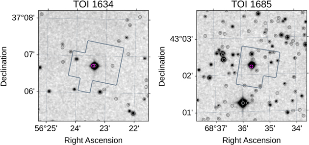
Figure 1. TESS photometric apertures and archival images for TOI-1634 (top) and TOI-1685 (bottom). The archival images are scanned photographic plates using the RG610 filter and the IIIaF emulsion, which were originally obtained as part of the POSSII-F survey on 1988 September 18 (TOI-1634) and 1989 October 6 (TOI-1685). The Gaia DR2 positions (epoch J2015.5) of the target stars are indicated by magenta circles and other sources by gray circles.

Download figure:
Standard image High-resolution imageTOI-1634 has a resolved companion star separated by 2 5 from the primary star (Gaia DR2 ID 223158499176634112), with a TESS magnitude of 14.368 ± 0.010 mag (i.e., about 3.3 mag fainter than TOI-1634). The Gaia astrometry indicates the companion star has a parallax of 28.62 ± 0.11 mas and proper motions of mas yr−1 and μδ
= 14.539 ± 0.091 mas yr−1, respectively (Gaia Collaboration et al. 2021), suggesting that TOI-1634 and the companion star share almost the same parallax and common proper motions. Thus, they are likely bound to each other, which was also reported in the visual-binary catalog for TOI's (Mugrauer & Michel 2020) as well as the more recent catalog by El-Badry et al. (2021) based on Gaia EDR3. Light-curve dilutions due to this companion star are taken into account when we perform the light-curve analyses. The impact of the companion on the estimation of the stellar properties as well as the long-term RV drift for TOI-1634 will be discussed in Sections 3.1 and 3.4. Other than this companion star, no stars were identified within in the Gaia EDR3 catalog having proper motions in common with TOI-1634 and TOI-1685.
5 from the primary star (Gaia DR2 ID 223158499176634112), with a TESS magnitude of 14.368 ± 0.010 mag (i.e., about 3.3 mag fainter than TOI-1634). The Gaia astrometry indicates the companion star has a parallax of 28.62 ± 0.11 mas and proper motions of mas yr−1 and μδ
= 14.539 ± 0.091 mas yr−1, respectively (Gaia Collaboration et al. 2021), suggesting that TOI-1634 and the companion star share almost the same parallax and common proper motions. Thus, they are likely bound to each other, which was also reported in the visual-binary catalog for TOI's (Mugrauer & Michel 2020) as well as the more recent catalog by El-Badry et al. (2021) based on Gaia EDR3. Light-curve dilutions due to this companion star are taken into account when we perform the light-curve analyses. The impact of the companion on the estimation of the stellar properties as well as the long-term RV drift for TOI-1634 will be discussed in Sections 3.1 and 3.4. Other than this companion star, no stars were identified within in the Gaia EDR3 catalog having proper motions in common with TOI-1634 and TOI-1685.


The signature of TOI-1634.01 was initially detected by the TESS SPOC in a transiting-planet search of sector 18 that occurred UT on 2019 December 12, yielding a 1.8R⊕ planet in a 0.98933 day orbit about its host star. The signal was detected at 10.6σ with an adaptive, noise-compensating matched filter (Jenkins 2002; Jenkins et al. 2010, 2020), passed all the diagnostic tests performed and published in the resulting Data Validation reports, and was fitted with a limb-darkened transit model (Twicken et al. 2018; Li et al. 2019). These included tests for eclipsing binaries, such as an odd/even depth test, a weak secondary test, and a ghost diagnostic test. The difference imaging centroid test showed that the source of the transit signature was consistent with the target star, TIC 201186294, with a measured offset from the target star of 81 ± 29 (we take 3σ as the confusion radius). The SPOC pipeline search removed the signature of TOI-1634.01 from the light curve and performed a search for additional transit signatures, which were not found. An alert for TOI-1634.01 was issued by the TESS Science Office (TSO) on UT 2020 January 14.
The signature of TOI-1685.01 was detected by the SPOC pipeline in a transiting-planet search of Sector 19 that occurred on UT 2020 January 17, resulting in a 1.47R⊕ planet in a 0.6669 day orbit. This transit signature passed all the diagnostic tests performed and reported in the Data Validation reports archived to MAST and the TSO alerted the community to this planet candidate on UT 2020 January 30. The difference imaging centroid test showed that the source of the transit signature was consistent with the target star, TIC 28900646, with a measured offset from the target star of 279 ± 266. As was done for TOI-1634, the SPOC pipeline removed the signature of TOI-1685.01 from the light curve and performed a search for additional transit signatures, which were not found. We note that these difference imaging centroid measurements are complementary to the high-resolution imaging reported in Section 2.2, which is limited to separations of 12 and 30 from each target.
We independently confirmed the transit signals of each planet candidate using a second-order polynomial Savitzy–Golay filter to remove stellar variability and instrumental systematics from each light curve, then used the transit least-squares algorithm (TLS; Hippke & Heller 2019) 45 to search them for transit signals, resulting in a signal detection efficiency (SDE) of 17.9, orbital period of 0.989 ± 0.003 days, and transit depth of 1.6 parts per thousand (ppt) for TOI-1634.01, and SDE of 18.6, orbital period of 0.669 ± 0.001 days, and transit depth of 1.0 ppt for TOI-1685.01. We subtracted each signal and repeated the transit search, but no additional transit signals with SDE above 10 were found in either light curve. TLS also reports the approximate depths of each individual transit; we note that these transit depths and uncertainties are useful for diagnostic purposes only, as they are simplistically determined from the mean and standard deviation of the in-transit flux. The depths of the odd transits are within 0.5σ of the even transits for both signals, suggesting a low probability of either signal being caused by an eclipsing binary at twice the detected period. These signals are consistent with those reported by the TESS team on ExoFOP-TESS. 46 The TLS detections are shown in Figure 2.

Figure 2. TLS transit signal detections for TOI-1634 (top) and TOI-1685 (bottom). The left panels show SDE vs. orbital period; the middle panels show the data folded on the detected period with the TLS model in blue, binned data in black; the right panels show the individual transit depths.
Download figure:
Standard image High-resolution image2.1.2. Okayama 188 cm/MuSCAT Photometry
We observed four transits of TOI-1685.01 on UT 2020 November 24, UT 2021 January 10, UT 2021 January 12, and UT 2021 January 14 using the multiband imager MuSCAT (Narita et al. 2015) mounted on the 188 cm telescope at Okayama Astro-Complex in Japan. MuSCAT has three channels for the g, r, and zs
bands, enabling three-band simultaneous imaging observations. Each channel is equipped with a 1024 × 1024 pixel CCD camera with a pixel scale of 036 pixel−1, which provides a field of view (FOV) of 6 1 square. We observed the target field with exposure times of 6–30 s depending on the band and sky condition. The obtained images were corrected for dark and flat in a standard manner, and aperture photometry was performed by a custom-built photometry pipeline (Fukui et al. 2011) to produce normalized light curves, in which the combinations of comparison stars and aperture radius were optimized such that the light-curve dispersion was minimized. The adopted aperture radius ranges from 8 to 14 pixels (from 29 to 51) depending on the band and night.
2.1.3. IAC 1.52 m/MuSCAT2 Photometry
We observed five transits of TOI-1634.01 on UT 2020 February 7, UT 2020 February 10, UT 2020 February 11, UT 2021 February 14, and UT 2021 February 16 using the multiband imager MuSCAT2 (Narita et al. 2019) mounted on the 1.52 m TCS telescope at Teide Observatory in Spain. MuSCAT2 is a sibling of MuSCAT but has four channels for the g, r, i, and zs
bands. The CCD cameras of MuSCAT2 are identical to those of MuSCAT, but the pixel scale is 044 pixel−1, which provides a FOV. The observations were conducted with exposure times of 3–60 s depending on the band and sky condition. The obtained data were reduced in the same way as for the MuSCAT data. We adopted aperture radii of 8–12 pixels (35–52) depending on the band and night, which means that the companion star at 25 away is contaminated into the photometric apertures in all bands.

2.1.4. FTN 2 m/MuSCAT3 Photometry
We observed one transit of TOI-1685.01 on UT 2021 February 1 using the brand-new multiband imager MuSCAT3 (Narita et al. 2020), which was installed on the 2 m Faulkes Telescope North (FTN) at Haleakala Observatory in Hawaii in late 2020. The telescope and instrument are operated by Las Cumbres Observatory. As with MuSCAT2, MuSCAT3 has four channels for the g, r, i, and zs
bands, but has wider format CCD cameras with a size of 2k × 2k. The pixel scale of each camera is 0266 pixel−1, which provides an FOV of 91 × 91. The observation was done slightly out of focus and with the exposure times of 25, 9, 8, and 20 s for the g, r, i, and zs
bands, respectively. The obtained raw images were processed by the BANZAI pipeline (McCully et al. 2018b) for dark and flat corrections, and then aperture photometry was performed in the same way as for the MuSCAT and MuSCAT2 data. The adopted radii of photometric aperture were 14, 18, 14, and 16 pixels (36, 47, 36, and 42) for the g, r, i, and zs
bands, respectively.
2.1.5. LCOGT Photometry
We observed a full transit of TOI-1634.01 on UT 2020 September 30 in Pan-STARRS z-short band and a full transit of TOI-1685.01 on UT 2020 November 11 in the Sloan band from the Las Cumbres Observatory Global Telescope (LCOGT) (Brown et al. 2013) 1.0 m network node at McDonald Observatory. We used the TESS Transit Finder, which is a customized version of the Tapir software package (Jensen 2013), to schedule our transit observations. The 4096 × 4096 LCOGT SINISTRO cameras have an image scale of 0389 per pixel, resulting in a field of view. The images were calibrated by the standard LCOGT BANZAI pipeline (McCully et al. 2018a), and photometric data were extracted with AstroImageJ (Collins et al. 2017). The TOI-1634.01 observation was slightly defocused and used 40 s exposures and a photometric aperture radius of 58 to extract the differential photometry, resulting in a photometric precision of ∼500 ppm model residuals in 5 minute bins. The TOI-1685.01 observation was mildly defocused and used 50 s exposures and a photometric aperture radius of 78 to extract the differential photometry, resulting in a photometric precision of ∼410 ppm model residuals in 5 minute bins.


2.1.6. OMM 1.6 m/PESTO Photometry
We observed a full transit of TOI-1685.01 at Observatoire du Mont-Mégantic, Canada, on UT 2020 March 8. The observations were made in the filter with a 15 s exposure time using the 1.6 m telescope of the observatory equipped with the 1024 × 1024 PESTO camera. PESTO has an image scale of 0466 per pixel, which provides an on-sky 795 × 795 FOV. The light-curve extraction via differential photometry was accomplished using an aperture radius of 70 and AstroImageJ. This software was also used for image calibration (bias subtraction and flat field division).

2.2. High-resolution Imaging
As part of the standard follow-up process, high-resolution imaging was performed to search for blended bound and unbound stellar companions and account for their presence in the analysis (e.g., Ciardi et al. 2015). Observations were performed with the optical speckle camera 'Alopeke on Gemini North for TOI-1634 and the near-infrared adaptive optics camera NIRC2 on Keck II for TOI-1685.
2.2.1. Gemini North/'Alopeke Speckle Observations
On UT 2020 December 2 TOI-1634 was observed with the 'Alopeke speckle imager (Scott 2019), mounted on the 8 m Gemini North telescope on Maunakea. 'Alopeke simultaneously acquires data in two bands centered at 562 nm and 832 nm using high-speed electron-multiplying CCDs (EMCCDs). We collected and reduced the data following the procedures described in Howell et al. (2011). The resulting reconstructed image achieved a contrast of Δmag = 8 at a separation of 1'' in the 832 nm band (see Figure 3). No secondary source was identified within 12 from TOI-1634.

Figure 3. 5σ contrast curves for TOI-1634 based on the Gemini North/'Alopeke Speckle Observations. The inset displays the reconstructed image of the target.
Download figure:
Standard image High-resolution image2.2.2. Keck II/NIRC2 Observations
We observed TOI-1685 with near-infrared (IR) high-resolution adaptive optics (AO) imaging at the Keck Observatory. We carried out the AO imaging using the NIRC2 instrument on Keck II behind the natural guide star AO system. The observations were made on UT 2020 September 9 in the standard three-point dither pattern that is used with NIRC2 to avoid the left lower quadrant of the detector, which is typically noisier than the other three quadrants. The dither pattern step size was set to 3'' and was repeated twice, with each dither offset from the previous dither by 05.
The observations were made in the narrowband Br − γ filter (λo
= 2.1686 μm; Δλ = 0.0326 μm) with an integration time of 1.5 s with one coadd per frame for a total of 13.5 s on target. The camera was in the narrow-angle mode with a full FOV of ≈ 10'' and a pixel scale of ≈ 000994 per pixel. The FWHM of the target in the combined image was ≈ 0052, and no additional stellar companions were detected in the 6'' × 6'' FOV (Figure 4).

Figure 4. Near-IR AO image of TOI-1685 taken with NIRC2 on Keck II and associated sensitivity curve. The black points represent the 5σ limits and are separated in steps of 1 FWHM ( ≈ 0052); the purple represents the azimuthal dispersion (1σ) of the contrast determinations (see text). The inset image is of the primary target showing no additional companions to within 3''of the target.
Download figure:
Standard image High-resolution imageThe sensitivities of the final combined AO image were determined by injecting simulated sources azimuthally around the primary target every 20° at separations of integer multiples of the central source's FWHM. Following, e.g., David et al. (2019), we computed the 5σ sensitivity limit as a function of the radial distance from the target. The near-IR AO sensitivity curve for TOI-1685 is shown in Figure 4 along with an inset image zoomed to the primary target showing no other companion stars.
2.3. Spectroscopy
2.3.1. TRES Spectroscopy
We obtained reconnaissance spectra of TOI-1634 on UT 2020 February 1 and UT 2020 September 4 and of TOI-1685 on UT 2020 February 2 and UT 2020 February 3 using the Tillinghast Reflector Echelle Spectrograph (TRES; Furesz 2008) located at the Fred Lawrence Whipple Observatory in Arizona, USA. TRES has a resolving power of ≈44,000 and a wavelength coverage of 385–910 nm, and the spectra were extracted as described in Buchhave et al. (2010).
RVs were determined from the TRES spectra using methods outlined in Winters et al. (2018). Briefly, molecular bands due to TiO in the wavelength range 7065–7165 Å found in aperture 41 of the TRES spectra were cross-correlated with an observed template spectrum of Barnard's Star (Gl 699). We conducted a search for maximum cross-correlation over a range of values of the rotational broadening applied to the template spectrum prior to correlation. As a result, we concluded there was no rotational broadening detectable in either target and therefore fixed the rotational broadening to zero for the final analysis. There is a systematic uncertainty in the velocity zero point of approximately 0.5 km s−1, which may be important when considering the absolute barycentric RV, rather than the relative velocity differences between the epochs. We obtained RV = −17.066 km s−1 (2020 February 1) and −17.105 km s−1 (2020 September 4) for TOI-1634, and RV = −43.306 km s−1 (2020 February 2) and −43.219 km s−1 (2020 February 3) for TOI-1685. For each target, the two spectra were secured at near opposite quadratures in the orbital phase based on the TESS ephemerides. Therefore, the absence of large RV variations ( ≳ 0.5 km s−1) ruled out stellar and brown-dwarf companions as the source of the transits for both targets.

2.3.2. Subaru/IRD Spectroscopy
For precise RV measurements of TOI-1634 and TOI-1685, we carried out near-IR observations of those two M dwarfs using Subaru/IRD between 2020 September and 2021 February under the Subaru IRD TESS intensive follow-up program (ID: S20B-088I). Every month during the period, we observed the two targets on two to three different nights when the program was assigned. On some of those nights, we visited the target stars twice within a night (two visits separated by a few hours) in order to mitigate the impact of the 1 day observing window, which happens to be close to the period of TOI-1634.01. IRD is a fiber-fed spectrograph placed in a temperature-stabilized chamber, which can simultaneously cover broadband near-IR wavelengths from 930 to 1740 nm with a spectral resolution of ≈ 70,000 (Tamura et al. 2012; Kotani et al. 2018). Stellar light collected by the telescope is first squeezed by the AO system on Subaru (Hayano et al. 2008), which is then injected into the spectrograph through a multimode fiber. For TOI-1634, the companion star at 25 was resolved in IRD's fiber injection module camera, and we ensured that only the primary (brighter) star was injected into the fiber. To trace the temporal instrumental stability, a secondary fiber is inserted into the spectrograph for simultaneous wavelength calibration, to which the laser-frequency comb (LFC) is usually injected. The integration times for both targets were set to 720–1200 s for each exposure, depending on the observing condition. We also observed at least one telluric standard star (A0 or A1 star) on each night to correct for the telluric lines in extracting the template spectrum for the RV analysis.
Raw IRD data were reduced by the standard procedure using IRAF (Tody 1993) as well as our custom codes to process the detector's bias and wavelength calibrations by LFC spectra (Kuzuhara et al. 2018; Hirano et al. 2020). The reduced one-dimensional spectra have a typical signal-to-noise ratio (S/N) of 60–95 per pixel at 1000 nm for both targets. Analyzing these reduced spectra, we extracted the RV for each frame. The RV analysis pipeline for IRD is described in Hirano et al. (2020); in short, individual observed spectra are first processed to create the stellar template spectrum, which is free from the telluric features and instrumental broadening. Using this stellar template as well as the instantaneous instrumental profile (IP) of the spectrograph (based on each LFC spectrum), each spectrum is fitted with the forward modeling technique. The typical RV internal errors are 3–4 m s−1 for both targets.
3. Analyses and Results
3.1. Estimation of Stellar Parameters
In this subsection, we will estimate the stellar parameters based on three independent methods. We then derive the most reliable stellar parameters jointly using those estimations.
3.1.1. Analysis of TRES Spectra
To estimate the basic stellar parameters, we independently analyzed the optical high-resolution spectra taken by TRES and near-IR spectra by IRD. For the TRES spectra, we made use of SpecMatch-Emp (Yee et al. 2017) to determine the effective temperature Teff, radius R⋆, and iron abundance [Fe/H] of the stars. The code attempts to fit an observed (input) high-resolution spectrum to a number of library spectra, whose stellar parameters were well determined, and find the best-matched stars in the library, by which the stellar parameters for the input spectrum are determined by interpolations. SpecMatch-Emp returned Teff = 3474 ± 70 K and 3468 ± 70 K, R⋆ = 0.435 ± 0.044 R⊙ and 0.417 ± 0.042 R⊙, and [Fe/H] = 0.13 ± 0.12 dex and 0.03 ± 0.12 dex, for TOI-1634 and TOI-1685, respectively.
3.1.2. Analysis of IRD Spectra
To estimate the atmospheric parameters for the two targets, we also analyzed the IRD spectra. Because many parts of the original IRD spectra suffer from significant telluric features (both absorptions and airglow emissions), we used the template spectra extracted for the RV analyses (Section 2.3), in which telluric features were removed and multiple frames were combined. The template spectra were then subjected to the analysis tool developed by Ishikawa et al. (2020). The analysis is based on a line-by-line comparison between the equivalent widths (EWs) from observed spectra and those from synthetic spectra. The synthetic spectra were calculated with a one-dimensional LTE spectral synthesis code that is based on the same assumptions as of the model atmosphere program of Tsuji (1978). For the atmospheric layer structure, we interpolated the grid of MARCS models (Gustafsson et al. 2008). The surface gravity and microturbulent velocity were needed to be assumed for the analysis. We referred to TIC for the values calculated from masses and radii (Stassun et al. 2019), which were estimated from the mass–MK relation in Mann et al. (2019) and the radius–MK relation in Mann et al. (2015), respectively. The microturbulent velocity was fixed at 0.5 ± 0.5 km s−1 for both objects for simplicity.


First, we used the FeH molecular lines in the Wing–Ford band at 990–1020 nm for the Teff estimation. The band consists of more than 1000 FeH lines, of which 57 lines with relatively clear line profiles were selected for the analysis. The adopted spectral line data are available from the MARCS web page. 47 We measured the EW of each FeH line by fitting the Gaussian profile and found the Teff at which the synthetic spectra best reproduce the EW by an iterative search. Throughout this first step, we assumed the solar value for the metallicity. The average of the Teff estimates for each of the 57 lines was taken as the best estimate here. Its uncertainty was given as the line-to-line scatter calculated by the standard deviation over the estimates from all the lines. Those procedures will be provided in more detail in Ishikawa et al. (2021, in preparation).
As a second step, adopting the Teff value estimated above, we determined the elemental abundances of Na, Mg, Si, Ca, Ti, Cr, Mn, and Fe from the corresponding atomic lines. The details of the abundance analysis are given in Ishikawa et al. (2020), although they adopted literature values for Teff. The spectral line data were taken from the Vienna Atomic Line Database (Kupka et al. 1999; Ryabchikova et al. 2015). We selected the lines based on three criteria: (1) not suffering from blending of other absorption lines, (2) sensitive to elemental abundances, and (3) continuum level can be reasonably determined. The EWs were measured by fitting synthetic spectra on a line-by-line basis. We searched for an elemental abundance until the synthetic EW matches the observed one for each line and took the average for all the lines to estimate [X/H] for an element X.
Subsequently, we adopted the iron abundance [Fe/H] determined in the second step as the metallicity of the atmospheric model grid to redetermine the Teff by the same procedure as in the first step. Then, we adopted the resulting Teff to finally determine the elemental abundances including [Fe/H] again in the same way as in the second step. The procedure up to this point allows the results of Teff and abundances to converge well within the measurement errors. Based on these analyses of IRD spectra, we obtained Teff = 3432 ± 99 K and 3428 ± 97 K and [Fe/H] = 0.27 ± 0.12 dex and 0.27 ± 0.12 dex for TOI-1634 and TOI-1685, respectively. The abundances for the other elements are listed in Table 1.
3.1.3. Analysis of Broadband Photometry
We also performed an analysis of the broadband spectral energy distribution (SED) of the star together with the Gaia EDR3 parallax (with no systematic offset applied; see, e.g., Stassun & Torres 2021) in order to determine an empirical measurement of the stellar radius, following the procedures described in Stassun & Torres (2016), Stassun et al. (2017), Stassun et al. (2018). We pulled the JHKS magnitudes from 2MASS (Skrutskie et al. 2006), the W1 – W4 magnitudes from WISE (Wright et al. 2010), the G, GBP, GRP magnitudes from Gaia (Gaia Collaboration et al. 2021), and the y-band magnitudes from Pan-STARRS (Flewelling et al. 2020). Together, the available photometry spans the full stellar SED over the wavelength range 0.4–20 μm (see Figure 5). We performed a fit using NextGen stellar atmosphere models, with Teff and [Fe/H] as the free parameters; the extinction AV was fixed at zero due to the proximity of the stars. Integrating the (unreddened) model SEDs gives the bolometric flux at Earth, Fbol. Finally, taking the Fbol and Teff together with the Gaia parallax gives the stellar radius, R⋆. The SED analysis provided Teff = 3500 ± 85 K and 3475 ± 75 K, [Fe/H] = 0.0 ± 0.5 dex and 0.0 ± 0.5 dex, Fbol = (7.64 ± 0.27) × 10−10 erg s−1 cm−2 and (6.65 ± 0.15) × 10−10 erg s−1 cm−2, and R⋆ = 0.466 ± 0.024 R⊙ and 0.473 ± 0.021 R⊙ for TOI-1634 and TOI-1685, respectively.

Figure 5. Spectral energy distributions of TOI-1634 (top) and TOI-1685 (bottom). Red symbols represent the observed photometric measurements, where the horizontal bars represent the effective width of the passband. Blue symbols are the model fluxes from the best-fit NextGen atmosphere model (black).
Download figure:
Standard image High-resolution image3.1.4. Joint Modeling of the Stellar Parameters
The three measurements (optical spectroscopy, near-IR spectroscopy, and SED fitting) of Teff and [Fe/H] yielded consistent results within their errors, and thus we computed the weighted means of those parameters to gain the final values (Table 1) used in the subsequent analyses. Because these measurements ultimately rely on similar stellar atmosphere models or the same calibration sources, we conservatively adopted the representative errors for the mean values of the two parameters (i.e., 70 K for Teff and 0.12 dex for [Fe/H]). Based on the basic parameters derived above, we further estimated the other stellar parameters (i.e., the stellar mass M⋆, radius R⋆, surface gravity , mean density ρ⋆, and luminosity L⋆), as well as refined the basic parameters (i.e., the stellar metallicity [Fe/H] and distance d) by combining all observed quantities in a consistent manner. In doing so, we took an approach described in Hirano et al. (2018), but with the inclusion of Gaia parallaxes; because the observed quantities are redundant (e.g., there are two sets of estimates for the stellar radius) and can be correlated with each other through the empirical relations, we performed Markov Chain Monte Carlo (MCMC) simulations in which the χ2 statistic of the likelihood function () is defined as


where and R⋆,SED, are the stellar radii estimated by the optical spectroscopy and SED integration, and and are their errors, respectively. The apparent Ks -band magnitude by 2MASS and its error are denoted by and , respectively. The fitting parameters in the MCMC analysis are the absolute Ks magnitude , stellar metallicity [Fe/H], and the distance d to the system. The modeled quantities R⋆ and in the right-hand side of Equation (1) are calculated from , [Fe/H], and d through the empirical relation by Mann et al. (2015) and . We assume AV = 0, given the proximity of the two stars to Earth. We imposed Gaussian priors on [Fe/H] and d based on the weighted mean value and its error for [Fe/H] derived above, and the Gaia parallax (Gaia Collaboration et al. 2021). In implementing the MCMC analysis, we computed M⋆ via the empirical relation of Mann et al. (2019) from and [Fe/H], as well as the surface gravity , the mean density ρ⋆, and the luminosity L⋆ for each step of the chain. For L⋆, we sampled the Teff values with the Gaussian distribution based on the values in Table 1.


TOI-1634 has a companion star 25 away from the primary star, but we were unable to identify the companion star in the 2MASS catalog. We inspected the 2MASS image for TOI-1634 and found that the companion star was buried in the point-spread function of the primary star, whose FWHM was found to be 27–28). This suggests that the Ks
magnitude listed in Table 1 may be contaminated by the companion star, and the true magnitude of the primary star could be slightly fainter. To roughly estimate its impact, we used the Dartmouth isochrone model (Dotter et al. 2008) and inferred the mass of the companion. Because the Dartmouth isochrones list the Gaia magnitudes as a function of stellar mass for a given set of stellar age and metallicity, we employed the Gaia GRP magnitude to constrain the companion's mass. The magnitude difference of ΔGRP = 2.959 between TOI-1634 and its companion translates to the companion's mass of ≈ 0.12 M⊙ on the assumption that TOI 1634's mass is roughly ≈ 0.46 M⊙. When those masses are adopted, the isochrones predict that the magnitude difference in the Ks
band should be mag, implying that the true of the primary star is ≈ 0.07 mag fainter than the reported one. With this in mind, we adopted instead of for TOI-1634 (in addition to shifting the center value of the magnitude, we conservatively added the systematic error of 0.07 in in quadrature) and ran the MCMC analysis. For TOI-1685, we directly input the 2MASS Ks
magnitude in the code. MCMC simulations were implemented using our custom code (e.g., Hirano et al. 2015) with a chain length of 106 after the burn-in chains. The final derived parameters based on this MCMC analysis (d, [Fe/H], , M⋆, R⋆, ρ⋆, and L⋆) are summarized in Table 1.


Using the Gaia EDR3 information as well as the absolute RVs from the TRES spectra, we also computed the Galactic space velocities (U, V, W) for the two stars with respect to the Sun (Table 1). The low space velocities for both targets indicate those stars belong to the thin disk. Velocity dispersions in the Galactic coordinate system are generally correlated with stellar age. Following the methodology described in Burgasser & Mamajek (2017), we computed the posterior distributions for the ages of the two stars. In doing so, we adopted the prescription given by Sanders & Binney (2015) for the velocity-dispersion evolution of the thin-disk stars with the Sun's peculiar velocity from Bland-Hawthorn & Gerhard (2016), and we used two different age priors: a uniform prior (0 < age ≤ 14 Gyr) and the age probability distribution in the Geneva–Copenhagen Survey (GCS) catalog (Casagrande et al. 2011). Based on the age posterior distributions, we found TOI-1634 has the age of Gyr (uniform prior) and Gyr (GCS prior) and that of TOI-1685 is Gyr (uniform prior) and Gyr (GCS prior), respectively. These results suggest the UVW velocities are not useful for constraining the ages of the two targets. We also confirmed that neither of the targets belong to nearby young associations based on the BANYAN Σ tool (Gagné et al. 2018).


3.2. Analysis of Transit Light Curves
We fit the TESS, MuSCAT, MuSCAT2, MuSCAT3, OMM, and LCO data sets using the PyMC3 (Salvatier et al. 2016), exoplanet 48 (Foreman-Mackey et al. 2019), starry (Luger et al. 2019), and celerite2 (Foreman-Mackey et al. 2017; Foreman-Mackey 2018) software packages. To account for systematics in the ground-based data sets we included a linear model of the covariates: airmass, pixel centroids, and the pixel response function peak and width. In addition, we included a Gaussian Process (GP; Rasmussen & Williams 2005) model to account for residual correlated noise not accounted for by the linear model, using a Matérn-3/2 covariance function. The transit model parameters we fit were: stellar mass and radius, quadratic limb-darkening parameters (two per bandpass), orbital period (P), time of transit center (Tc ), planet to star radius ratio (Rp /R⋆), and impact parameter (b). We assumed a circular orbit and placed Gaussian priors on the stellar mass and radius based on the results in Table 1. We also placed Gaussian priors on the limb-darkening coefficients based on the interpolation of the parameters tabulated by Claret et al. (2012) and Claret (2017), propagating the uncertainties in the stellar parameters in Table 1 via Monte Carlo simulations.
We used the gradient-based BFGS algorithm (Nocedal & Wright 2006) implemented in scipy.optimize to find initial maximum a posteriori parameter estimates. We used these estimates to initialize an exploration of parameter space via "no U-turn sampling" (Hoffman & Gelman 2014), an efficient gradient-based Hamiltonian Monte Carlo sampler implemented in PyMC3. We first conducted a fit to the TESS data using a window centered on each transit of width three times the full transit duration (3 × T14), including a local linear time baseline function for each window to account for stellar variability. The folded TESS data and best-fit transit models are shown in Figures 6 and 7. We then fit each of the ground-based transit data sets using Gaussian priors derived from the impact parameter and orbital period posteriors of the TESS fit, in addition to the stellar mass, radius, and limb-darkening priors. We assumed an achromatic transit model and shared the GP hyperparameters between photometric bands taken simultaneously by MuSCAT1/2/3. Examples of the ground-based data and model fits for the various instruments used in this work are shown in Figures 8, 9, and 10. Due to the increased photometric scatter of the target stars in bluer bandpasses, we performed tests to determine whether the precision of our ground-based simultaneous multiband transit measurements could be improved by using only the redder bandpasses. Despite the relatively low S/N of the transit signal in the g band, for the data set shown in Figure 8, we found that excluding g band from the fit (i.e., using only r, i, and zs bands) resulted in 18% worse precision in Tc , and 11% worse precision in Rp /R⋆. Similarly, we found that excluding both g and r bands from the fit resulted in 55% worse precision in Tc and 43% worse precision in Rp /R⋆. We thus opted to include all bands in our fits in order to take advantage of the maximum precision afforded by our data sets. Finally, we computed a weighted mean of the measurements of Rp /R⋆ from each data set and used the individual transit time posteriors to compute a linear orbital ephemeris and search for transit timing variations; the resulting parameter estimates are listed in Table 2.

Figure 6. Phase-folded TESS photometry with transit model for TOI-1634.01 (top) and the residuals from the fit (bottom).
Download figure:
Standard image High-resolution image
Figure 7. Same as Figure 6 but for TOI-1685.01.
Download figure:
Standard image High-resolution image
Figure 8. MuSCAT2 photometry of TOI-1634.01 taken on UT 2020 February 11. The upper row shows the raw photometry with full systematics and transit model in each bandpass, the middle row shows the systematics-corrected photometry with only the transit model, and the bottom row shows the residuals from the fit.
Download figure:
Standard image High-resolution image
Figure 9. Same as Figure 8, but for the MuSCAT3 photometry of TOI-1685.01 taken on UT 2021 January 30.
Download figure:
Standard image High-resolution image
Figure 10. Same as Figure 8, but for the OMM (left) and LCO (right) photometry of TOI-1685.01 taken on UT 2020 March 8 and November 11, respectively.
Download figure:
Standard image High-resolution imageTable 2. Planetary Parameters of TOI-1634b and TOI-1685b
| Parameter | TOI-1634b | TOI-1685b |
|---|---|---|
| Transit parameters | ||
| P (days) | 0.9893436 ± 0.0000020 | 0.6691416 ± 0.0000019 |
| Tc (BJD-2457000) | 1791.51495 ± 0.00053 | 1816.2255 ± 0.0011 |
| b | 0.375 ± 0.049 | 0.416 ± 0.053 |
| Rp /R⋆ | 0.0356 ± 0.0010 | 0.0291 ± 0.0010 |
| Derived parameters | ||
| Rp (R⊕) | 1.749 ± 0.079 | 1.459 ± 0.065 |
| Mp (M⊕) | 10.14 ± 0.95 | 3.43 ± 0.93 |
| ρp (g cm−3) | ||
| a (au) | 0.01490 ± 0.00017 | 0.011557 ± 0.000092 |
| io (deg) | 86.98 ± 0.41 | 85.59 ± 0.58 |
| Teq (AB = 0) (K) | 920 ± 25 | 1052 ± 26 |
| Teq (AB = 0.3) (K) | 842 ± 23 | 962 ± 24 |


Download table as: ASCIITypeset image
3.3. Rotation Analysis
As a last piece of the light-curve analysis, we performed a periodogram analysis on the TESS light curves for both targets to search for possible rotational modulations. The rotation period is one of the basic parameters to characterize the host star, which is also useful to disentangle the real planetary signal from the stellar activity in modeling the observed RV variations (e.g., Grunblatt et al. 2015; Barragán et al. 2019). We calculated the generalized Lomb-Scargle (GLS) periodograms (Zechmeister & Kürster 2009) for the TESS light curves of TOI-1634 and TOI-1685 corrected for systematics using pixel level decorrelation (PLD; Deming et al. 2015), as implemented in the lightkurve package (Lightkurve Collaboration et al. 2018). The SPOC pipeline removes instrumental correlated noise from the TESS light curves, but it can also remove astrophysical signals; we opt to use PLD instead, as it can correct systematics while preserving signals of interest, such as starspot modulation. Figures 11 and 12 show the PLD light curves after binning (1 bin = 0.1 days) as well as the GLS periodograms for TOI-1634 and TOI-1685, respectively. Both light curves exhibit low-frequency modulations likely induced by surface spots, but in both cases the periodicity is ambiguous due to the short observing windows. The period of TOI-1634 could be around 24.8 days based on the GLS peak and visual inspection, but it may correspond to a multiple of the true rotation frequency. For TOI-1685, the light curve and periodogram indicate the rotation period of the star is much longer than the observing window (i.e., Prot ≳ 30 days).

Figure 11. PLD-corrected binned TESS light curve for TOI-1634 (upper panel) and its GLS periodogram (bottom panel).
Download figure:
Standard image High-resolution image
Figure 12. PLD-corrected binned TESS light curve for TOI-1685 (upper panel) and its GLS periodogram (bottom panel).
Download figure:
Standard image High-resolution imageWe also inspected the photometric data from the All-Sky Automated Survey for Supernovae (ASAS-SN: Shappee et al. 2014; Kochanek et al. 2017), which recorded the magnitudes of target stars for more than five years. However, both GLS periodograms for TOI-1634 and TOI-1685 show no meaningful peak (False Alarm Probability: FAP < 1.0%), likely due to the low photometric precision (≈1.5%–2.0%) compared to the variability amplitude by stellar rotation (typically less than 0.01 mag: Newton et al. 2016; Medina et al. 2020). Unfortunately, available photometric data did not allow us to pin down the accurate rotation periods for TOI-1634 and TOI-1685, but we confirmed that both targets are slowly rotating stars with Prot ≳ 25 days from the TESS light curves. This lower limit on Prot corresponds to an upper limit of ≈0.90–0.92 km s−1 on for both stars.

The slow rotation of the two targets indicates that they are relatively old M dwarfs. The old ages are also corroborated by the lack of an emission line in the chromospheric activity indicators. For instance, we inspected the Hα line in the TRES optical spectra for both targets and found that they have the Hα "absorption" line with no sign of emission at the line core. Such an absorption feature at Hα for an M3 dwarf implies that the stellar age is likely older than a few Gyr (see, e.g., Figure 6 of Kiman et al. 2021) and the star has a long rotation period (e.g., Newton et al. 2017). This is also consistent with the lack of flares in the TESS light curves, whose rate provides a good indicator for the stellar age of mid-to-late M dwarfs (Medina et al. 2020).
3.4. Period Analyses and Orbital Fits
In this subsection, we describe the period analyses and orbital fits to the RV data obtained by Subaru/IRD.
3.4.1. TOI-1634
The planetary transit was securely detected in the light curves by the ground-based photometry (Figure 8), in which the observed transit depths were consistent with the TESS photometry. However, the companion star at 25 was inside the photometric aperture
49
, meaning that the ground-based photometry alone was not capable of ruling out the possibility that the transits are originating from the companion star (companion's flux contamination is larger than the transit depth). In order to check if our RV data alone indicate the presence of the USP planet around TOI-1634, we performed a period analysis using the GLS tool (Zechmeister & Kürster 2009) applied to the observed IRD-RV data. The upper panel of Figure 13 shows the GLS periodogram for TOI-1634's raw RV data. There are multiple peaks with very low FAPs (<0.1%), but the highest peak shows up at the correct period of the transiting planet (P = 0.989 days), which does not fall on the peaks of the window function (blue-shaded area). Therefore, our RV data indicate additional, independent evidence of the USP planet orbiting TOI-1634 and not orbiting its companion star.

Figure 13. GLS periodograms for TOI-1634. The upper panel displays the periodogram in red on the original RV data. The GLS periodogram computed for the residual RV data after subtracting the best-fit Keplerian motion by the USP planet (TOI-1634b) is shown in the lower panel. In both panels, the window functions are shown by the blue-shaded regions. The highest peak in the upper panel, indicated by the green arrow, precisely matches the correct period of TOI-1634b (P = 0.989 days).
Download figure:
Standard image High-resolution imageNext, we attempted the orbital fit to the observed RVs. In doing so, we first estimated the impact of the companion star around TOI-1634; given the proximity to the star, the companion star at 25 away might have a nonnegligible impact on the long-term RV baseline. With the distance of d = 35 pc for TOI-1634, the angular separation of 25 translates to the projected separation of 88 au, which approximately sets the lower limit to the semimajor axis of the binary orbit except for a highly eccentric orbit (i.e., abinary ≳ 88 au). The RV acceleration of the primary star () around the center of mass of the system is expressed as


where G is the gravitational constant, Mcomp is the companion star's mass, io is the orbital inclination, f is the true anomaly, e is the orbital eccentricity, and ω is the argument of periastron. When we assume the companion's mass of ≈0.1 M⊙ (see Section 3.1) and e = 0 for the binary orbit, the lower limit on abinary gives the maximum RV acceleration as

In the presence of moderate eccentricity, the upper limit of could be a few times larger than the above value, depending on the orbital phase. Hence, this order-of-magnitude estimation suggests that the stellar companion may lead to an RV drift of up to a few m s−1 over the course of ≈5 months.

We constrained the visual-binary orbital parameters using the LOFTI_gaiaDR2 software package (Pearce et al. 2020). LOFTI_gaiaDR2 uses the instantaneous positions, proper motions, and masses of the components of visual-binary stars to estimate their orbital parameters. We used the astrometric parameters from Gaia EDR3 for this calculation, along with the stellar masses for the primary and secondary stars estimated in Section 3.1. The LOFTI_gaiaDR2 posterior probability distribution has a slight preference for highly eccentric solutions (68% confidence interval between e = 0.61 and 0.98) but remains consistent with circular orbits. We note that these parameters should be taken with some skepticism because the astrometric solution for the secondary star shows excess scatter (with a Renormalized Unit Weight Error, or RUWE, of 1.7), which can indicate that it is itself an unresolved binary companion that can significantly affect its proper motion. Regardless, we conclude that the Gaia positions and proper motions are not inconsistent with an eccentric visual binary orbit.
Based on these speculations, we modeled the observed RVs of TOI-1634 using the following equation, in which we allow for the presence of a possible RV trend:

where K is the RV semiamplitude and γ is the RV offset of our data set. The time t0 is an arbitrary origin of time for which we adopt the time of the first RV point in the whole data set. We optimized the orbital parameters (K, , , γ, ) using MCMC (Hirano et al. 2015) with uniform priors for all parameters. In the fit, we fixed P and Tc based on the transit ephemeris (Table 2).


We attempted the orbital fits assuming both circular and eccentric orbits. The results of those fits are shown in Table 3 ("with " columns). To discuss the significance of the nonzero eccentricity, we compared the Bayesian Information Criterion (BIC), which is computed by , where k is the number of fitting parameters and N is the number of data points. Comparing the two BIC values for the above solutions, we found ΔBIC = BICe=0 − BICe≠0 = 1.5, implying that the circular and eccentric orbital solutions are almost equally favored. In other words, no evidence for nonzero eccentricity is found in our data set. A near-zero orbital eccentricity is also expected from the tidal circularization timescale for USP planets; using Equation (17) of Patra et al. (2017) with the planetary tidal quality factor of Qp ≈100 (for a terrestrial planet) (e.g., Ment et al. 2021), we obtain the tidal damping timescale of ≈5.5 × 10⁴ yr for TOI-1634b, implying that a nonzero eccentricity should have been damped in the past. Therefore, we concluded that the TOI-1634b has an almost circular orbit and adopt the fitting result for e = 0 in the subsequent analysis. The RV data and the best-fit orbital solution to the data are plotted in panels (a) and (b) of Figure 14.


Figure 14. Observed RV variations for TOI-1634. (a) The original RVs are plotted as a function of BJD, along with the best-fit model including a linear RV trend (e = 0). (b) Phase-folded RV curve for TOI-1634b after subtracting the linear RV trend. The best-fit models with the circular and eccentric orbits are drawn by solid (red) and dashed curves, respectively. (c) Phase-folded RV curve assuming no RV trend is present () in the data. The best-fit model for e = 0 is shown in red.

Download figure:
Standard image High-resolution imageTable 3. Results of the Orbital Fits
| TOI-1634b | TOI-1685b | |||||
|---|---|---|---|---|---|---|
| Parameter | with (e = 0)⋆ | with (e ≠ 0) | no (e = 0) | with Feb-02 (e = 0) | no Feb-02 (e = 0)⋆ | no Feb-02 (e ≠ 0) |
| K ( m s−1) | 11.1 ± 1.0 | 11.31 ± 0.99 | 11.80 ± 0.91 | 3.3 ± 1.1 | 4.2 ± 1.1 | |
| 0 (fixed) | 0 (fixed) | 0 (fixed) | 0 (fixed) | 0.278 ± 0.076 | ||
| 0 (fixed) | 0 (fixed) | 0 (fixed) | 0 (fixed) | |||
| (m s−1 day−1) | −0.023 ± 0.012 | −0.023 ± 0.012 | 0 (fixed) | 0 (fixed) | 0 (fixed) | 0 (fixed) |
| BIC | 70.6 | 69.1 | 70.0 | 54.4 | 43.1 | 39.0 |


Note. For each planet, the fitting result adopted to compute the planet mass is indicated by ⋆.
Download table as: ASCIITypeset image
The best-fit RV acceleration is ≈3 times larger than the value in the right-hand side of Equation (3), but it is consistent with zero within 2σ. While this possibly large RV drift might be attributed to a moderate eccentricity of the binary orbit as discussed above, it could be an artifact caused by a small number of RV points around the beginning and/or end of our observing campaign spanning ∼5 months. Given the frequency of planet multiplicity for USP planets (Winn et al. 2018), it is also possible that there exists an outer planet in the system that gave systematic offsets at specific orbital phases for the inner USP planet. To discuss the significance of this RV trend, we next fitted the observed RV data in the absence of the RV trend assuming a circular orbit. Our MCMC analysis suggested K = 11.80 ± 0.91 m s−1, which is compatible with the result in the presence of . Comparing the BICs for the two fitting results, we found that the result without the trend is equally likely (). We thus list both fitting results (with and without ) in Table 3 to take into account the uncertainty of the systematic RV offset. We employ the result with and e = 0, which is physically motivated from the dynamics of the system, in deriving the planet mass Mp as well as the mean density ρp from K (Table 2).


After removing the best-fit orbital model (e = 0, ) for the observed RV data, we performed an extra periodogram analysis to search for additional planets in the system. The bottom panel of Figure 13 illustrates the GLS periodogram (red solid line) for the residual RV data. No significant peak was found in the residual RVs, suggesting either that no additional massive planet is present in the system with a period shorter than our observation span or that the signal of such unidentified planets was removed/minimized by the orbital fit of TOI-1634b and long-term RV trend. At this point, our RV data imply no evidence for additional planets in the system.

3.4.2. TOI-1685
We ran a period analysis for the observed RV of TOI-1685 in a similar manner to TOI-1634. The upper panel of Figure 15 plots the GLS periodogram for the raw RV data. There are several significant peaks exceeding the FAP = 0.1% line, but the one at the period of TOI-1685b (P = 0.669 days) is not high enough to claim the detection of the orbital signal. After a preliminary orbital fit to the observed RV data using the transit ephemeris, we found that the RV points taken on UT 2021 February 2 (hereafter "Feb-02") are the primary outliers, deteriorating the fitting result for the planet. Although this could be indicative of the presence of an additional planet in the system, we also suspected that this sudden RV shift is caused by an instrumental systematic. The IRD spectrograph is known to exhibit a relatively large temporal RV drift, which is well correlated with the temperature instability at the camera lens inside the chamber (Kotani et al. 2018; Hirano et al. 2020). This instrumental RV drift is usually corrected by modeling the instantaneous IP of the spectrograph derived from the simultaneously taken wavelength-reference spectrum (i.e., LFC). However, if the variation in the IP is too fast compared to each integration time, it is theoretically expected that the LFC is unable to accurately trace the "effective" instantaneous IP of the spectrograph.

Figure 15. GLS periodograms (red solid lines) for TOI-1685's RV data with (upper panel) and without (lower panel) the Feb-02 data. As in Figure 13, blue-shaded areas indicate the window function. The black horizontal lines correspond to FAPs indicated in the plot. The period of TOI-1685.01 is denoted by the green arrow in both panels.
Download figure:
Standard image High-resolution imageTo further investigate this possibility, we inspected the absolute instrumental drift of the spectrograph on February 2 and found that the IRD spectrograph indeed exhibits a large instrumental instability that night as shown in Figure 16. In particular, TOI-1685 was observed at the very beginning of the night (blue squares), when the instrumental RV variation was most significant; the spectrograph exhibits an RV drift of ≈8 m s−1 for every integration. 50 In addition, the observing condition during the twilight usually changes dramatically, and thus the combination of instrumental instability and variations in the twilight observing conditions may have affected the extraction and application of the effective IPs from the LFC spectra.

Figure 16. Temporal RV drift of IRD spectra on UT 2021 February 2, measured based on the emission lines of the LFC spectra. This apparent RV drift is caused by the temperature instability of the spectrograph.
Download figure:
Standard image High-resolution imageThe impact of IRD's instrumental RV drift, especially for the case of relatively long integrations, is under investigation, and therefore we decided to perform the orbital fits with and without including the Feb-02 data. We first computed the periodogram for the data set excluding the Feb-02 data. The lower panel of Figure 15 plots the resulting GLS periodogram. While the same peaks (FAP < 0.1%) identified for the original data set (upper panel) have similar GLS powers, the peak at the correct period of TOI-1685b (P = 0.669 days) now appears with a low FAP (<0.1%); whether instrumental or astrophysical, the absence of a significant peak at TOI-1685b's orbital period in the original periodogram is ascribed to the inclusion of the Feb-02 data. The two peaks around 0.70 and 0.72 days in Figure 15, which are higher than the 0.67 day peak, are likely aliases associated with the peak at 2.59 days. The window function has peaks at 1.0 day and 0.96 days (the highest and second-highest ones for P<10 days). When those window frequencies are coupled with the period at 2.59 days, the periodogram would exhibit alias peaks around 0.72 and 0.70 days, respectively. The 2.59 day periodicity will be discussed later.
For the RV data with and without the Feb-02 data, we next fitted the observed RVs with a single-planet model. Assuming either a circular or eccentric orbit, we performed the MCMC analysis as in the case of TOI-1634 for each data set. When the Feb-02 data were included, we obtained K = 3.3 ± 1.1 m s−1 and m s−1 for the circular and eccentric orbits, respectively. The two fitting results yielded ΔBIC = BICe=0 − BICe≠0 = −2.3, implying that the circular orbit is slightly favored for this data set. We obtained larger K values in the absence of the Feb-02 data: K = 4.2 ± 1.1 m s−1 and m s−1 for e = 0 and e ≠ 0, respectively. In this case, the two fits resulted in ΔBIC = BICe=0 − BICe≠0 = +4.0; unlike the case with the Feb-02 data, an eccentric orbit is a slightly favorable solution. Note that as in the case of TOI-1634, the tidal circularization timescale for TOI-1685.01 is estimated as ≈1.0 × 10⁴ yr for Qp ≈100 (Earth-like rocky planet), indicating that e should be vanishingly low in the absence of an additional planet in the system. Those fitting results are shown in Table 3 and the phase-folded RVs are plotted in Figure 17. For the final planet mass Mp (Table 2), we adopt the K value for the case of e = 0 without the Feb-02 data.


Figure 17. Results of the RV fits for TOI-1685 with a single-planet model (a) with and (b) without the inclusion of the Feb-02 data. The blue points are observed RV data, and the red solid line indicates the best-fit circular model in each panel. In panel (b), we show the best-fit eccentric orbit with the dashed line. In both panels, the RV residuals from the best-fit circular orbit are plotted at the bottom.
Download figure:
Standard image High-resolution imageIn order to search for an additional signal in the observed RV data, we computed the periodogram for TOI-1685's RVs after removing the best-fit single-planet model for each data set. Considering the short tidal circularization timescale for the USP planet, we removed the circular-orbit solutions derived above. Figure 18 plots the GLS periodograms for the whole RV data and the data subset without the Feb-02 data. For both panels, there are a few significant peaks (FAP<0.1%) that do not fall in the window function. The peak at 2.6 days is common to both periodograms, which was also seen in the original RVs without the Feb-02 data (lower panel of Figure 15). The high peaks at P<1.0 day in both panels are likely alias peaks associated with the 2.6 day peak and window functions.

Figure 18. GLS periodograms computed for TOI-1685's residual RV data after subtracting the best-fit Keplerian motion by the USP planet (TOI-1685.01). The results with and without the Feb-02 data are shown in the upper and lower panels, respectively. The 2.6 day periodicity discussed in the text is shown by the orange arrow in each panel.
Download figure:
Standard image High-resolution imageGiven the limited phase coverage and unknown instrumental systematics, at this point we are not able to claim that the 2.6 day periodicity in the RV data represents an additional planet in the system; more RV measurements are essentially required to gain a robust conclusion on the presence of an additional body in the system. Nonetheless, we were tempted to fit the observed RV data with a two-planet model. In doing so, we ran the MCMC code and fitted the RV data (with and without the Feb-02 data) assuming two circular Keplerian orbits. We fixed the period of the USP planet at the one from the transit ephemeris and allowed the period of the outer planet P2 and time of the inferior conjunction Tc,2 to float with uniform priors. The results of these fits are listed in Table 4. In the table, K1 and K2 represent the RV semiamplitudes for the inner (USP) and outer planets, respectively. The phase-folded RV curves (with the inclusion of Feb-02 data) after removing the Keplerian orbit for the other planet are shown in Figure 19. The RV semiamplitudes for the USP planet are consistent within ≈1σ with the values derived for the one-planet model (Table 3) in both cases, whereas the RV scatters around the best-fit models significantly improved with ΔBIC = BICone−planet − BICtwo−planet being greater than 10 for both fits.

Figure 19. The result of the RV fit for TOI-1685 with a two-planet model. Phase-folded RV curves for the USP planet (upper panel) and the outer one (lower panel) are respectively shown after subtracting the best-fit Keplerian orbit for the other planet.
Download figure:
Standard image High-resolution imageTable 4. Results of the Orbital Fits for TOI-1685 with a Two-planet Model
| Parameter | with Feb-02 Data | no Feb-02 Data |
|---|---|---|
| K1 ( m s−1) | ||
| K2 ( m s−1) | 6.2 ± 1.0 | |
| P2 (days) | ||
| Tc,2 (BJDTDB) |


Download table as: ASCIITypeset image
We note that the 2.6 day signal is unlikely to be explained by stellar rotation. If the rotation period of the star is Prot = 2.6 days, the equatorial rotation velocity must be ≈8.8 km s−1, which also gives the projected rotation velocity for the case of spin–orbit alignment in the system. Both TRES optical spectra and IRD near-IR spectra, however, imply that the star is slowly rotating with km s−1. The slow rotation of TOI-1685 is also supported by the low-frequency light-curve modulation as discussed in Section 3.2. Therefore, we conclude that the 2.6 day periodicity does not indicate the rotational signal in the RV data, but represents any one of (1) an additional planet, (2) an instrumental/analysis artifact, or (3) an artifact caused by the mixture of (1) and (2) as well as the window function of our IRD observations. Again, further observations are required to test those possibilities.


If the 2.6 day signal indeed represents the period of the outer planet, K2 ≈6 m s−1 corresponds to the planetary mass of . Although the two planets in the system have relatively small masses, the small orbital separation between the two planets prompted us to check for the orbital stability of the two planets. Because the outer one is not transiting and its orbital inclination (thus the true mass) is not known, currently there is little point in running detailed numerical simulations for the system. Instead, we simply compared the minimum separation between the two in terms of the mutual Hill sphere RH, following Pu & Wu (2015). Inputting the semimajor axes of the two planets (a1 = 0.0116 au and a2 = 0.0285 au for the inner and outer planets, respectively) on the assumption that the planets are coplanar, we found RH ≈0.00058 au. Thus, the minimum separation between the two planets (a2 − a1 = 0.0169 au) is about 29 times larger than the mutual Hill radius. Pu & Wu (2015) showed that if the minimum separation is larger than ≈12 RH, the system should be stable on a billion-year timescale. Also considering that the periods of the two planets are not near a first-order mean-motion resonance, the addition of a super-Earth-mass planet at P = 2.6 days does not critically deteriorate the stability of the system.

4. Discussion
4.1. Planet Compositions
Based on the results of light-curve analyses and RV fits, we estimated the physical parameters of the planets, including the mass Mp , radius Rp , semimajor axis a, and equilibrium temperature Teq assuming zero albedo (AB = 0) as well as Earth-like albedo (AB = 0.3), which are listed in Table 2. In computing Teq, we assumed a constant temperature across the entire planet. To plot the two planets in the mass–radius (MR) diagram for exoplanets, we downloaded the catalog of transiting planets from the TEPcat database (Southworth 2011) and used the mass and radius of well-characterized planets, with the precisions on both measurements better than 30%. Figure 20 shows the MR diagram, focusing on relatively small-sized planets with Rp <3.0 R⊕. The blue and purple points in the figure indicate the USP planets in the literature, while the gray ones are other longer-period planets. In the same figure, MR curves for different planet compositions are drawn based on the theoretical MR relations by Zeng et al. (2016, 2019). For models including water and/or hydrogen atmosphere, a surface temperature of 1000 K is assumed in the plot based on the equilibrium temperature of the planets in Table 2. Models including water-rich cores with hydrogen envelopes are not shown in the figure, as the radii of such planets usually exceed 3.0 R⊕ even with the smallest addition of hydrogen envelope (i.e., 0.1% of H2).

Figure 20. MR diagram for known transiting planets (Rp <3.0 R⊕) as well as our new planets (blue squares). The catalog was downloaded from the TEPcat database (Southworth 2011) and theoretical models are drawn based on Zeng et al. (2016, 2019). USP planets around M dwarfs (except our new planets) and FGK stars are shown in purple and blue, respectively.
Download figure:
Standard image High-resolution imageThe derived mean densities for TOI-1634b and TOI-1685b are g cm−1 and g cm−1, respectively, which are higher than that of Earth. All the USP planets plotted in Figure 20 including our new planets TOI-1634b and TOI-1685b have interior compositions consistent with Earth's composition (i.e., 32.5% Fe + 67.5% MgSiO3) or pure rock (which is only allowed for TOI-1685b), and the diagram implies that it is very unlikely that the two planets possess light element (H–He) rich atmospheres. Among the USP planets plotted in the diagram, TOI-1634b is one of the largest and most massive planets having Earth-like compositions. The radius of TOI-1634b falls near the radius gap of super-Earths (Fulton et al. 2017), which makes the planet a benchmark for a population of large USP planets around low-mass stars; residing near the radius gap, TOI-1634b is useful in the context of discussing to what extent the rocky cores of close-in planets can grow and how such large planets were delivered to the present locations and lost their volatile-rich envelopes. TOI-1685b is more like a typical USP planet with Rp ≲ 1.5 R⊕, whose composition is consistent with Earth.


4.2. Atmospheric Escape from the USP Planets
Our finding that both TOI-1634b and TOI-1685b are almost "bare" planets having little, if any, volatile-rich atmosphere is corroborated in the context of the photoevaporation theory, independently of the observed mean densities. Atmospheric escapes are generally driven by several physical processes (e.g., Tian 2015). USP planets having massive atmospheres are in danger of tidal disruption. If TOI-1685 b initially had a primordial atmosphere of ≳10%–20% of its total mass at the current location, the atmosphere should have been blown off instantaneously by the Roche lobe overflow because of its small core mass and a high equilibrium temperature, whereas the more massive TOI-1634b has never experienced Roche lobe overflow if it initially had such a massive atmosphere. The observed MR relationship, however, rules out the presence of such a massive atmosphere on the two USP planets.
The primordial atmosphere on a USP planet is exposed to intense stellar irradiation and high-energy charged particles from a stellar wind and coronal mass ejection. In particular, the hydrodynamic escape driven by high-energy (X-ray and extreme UV: XUV) photons from the host star (e.g., Sekiya et al. 1980; Watson et al. 1981) plays a crucial role for highly irradiated close-in planets (Owen 2019). We simulated the long-term evolution of TOI-1634 b and 1685 b that initially have the atmospheric mass fraction of ≲a few percent on an Earth-like core under strong stellar XUV irradiation. We used the physical properties of the two USP systems given in Tables 1 and 2. We adopted the XUV flux model for M dwarfs given in Jackson et al. (2012), where the bolometric luminosities of TOI-1634 and 1685 were assumed to be their current values. The hydrodynamic mass loss from a planet with a H2–He atmosphere is calculated by

where η is the heating efficiency by stellar XUV irradiation, LXUV is the stellar XUV luminosity, Rp is the planetary radius, a is the semimajor axis of the planet, G is the gravitational constant, and Ktide is the potential energy reduction factor due to the stellar tidal effect (Erkaev et al. 2007). We adopted η = 0.1 for low-mass planets as suggested in Owen & Jackson (2012). The planetary radius, which is defined as the location at which a H2–He atmosphere becomes optically thick to stellar XUV photons, can be determined by the thermal evolution of the planet (see also Hori & Ogihara 2020 for detailed numerical prescriptions).
The two USP planets are expected to completely lose their primordial (i.e., H- and He-rich) atmospheres by photoevaporation within ≲1 Gyr, which are also consistent with the mass-loss timescales given in Owen & Wu (2017) (see Equation (20)). Although the precise ages of TOI-1634 and TOI-1685 are not well determined, the two USP systems exhibit no signs of particular youth (e.g., rapid rotation and high surface activity). Thus, once the USP planets accreted a primordial atmosphere of ≲a few wt% from the protoplanetary disk, all the atmospheres are likely to be lost by photoevaporation processes. Hence, both planets should be bare planets, similar to the other known USP planets.
4.3. Further Follow-up Studies
As discussed above, TOI-1685's RV data exhibit an extra scatter when fitted with a single-planet model, which could be attributed to the presence of an additional planet or activity-/instrument-induced systematic effects. More RV observations are beneficial not only to confirm or rule out the presence of an outer planet but also to obtain an accurate mass for the USP planet; in the presence of unknown additional bodies in the system, the mass measurement of a known transiting planet is more or less affected by systematic variations due to additional bodies. Therefore, the planet masses given in Table 2 and Figure 20 are tentative ones, whose systematic errors might be underestimated. We note that in many theoretical scenarios of the USP planet formation, outer planets play a key role in bringing the USP planets to the current locations (e.g., Schlaufman et al. 2010; Pu & Lai 2019; Millholland & Spalding 2020). Additional RV monitoring would be able to uncover the architecture of the two systems up to a larger orbital distance. Specifically, once an outer planet is confirmed beyond the USP planet, properties such as the period ratio, orbital eccentricity, and mutual inclinations would be valuable clues to test the formation scenarios of USP planets.
The brightness of TOI-1634 and TOI-1685 also makes them excellent targets for future follow-up studies, including atmospheric characterizations. As discussed in Section 4.2, the primordial H–He atmosphere of the UPS planets would have been lost due to strong irradiation of high-energy photons from the host stars. However, the planets may still hold a geometrically thin layer of atmosphere composed of heavy elements, formed, e.g., by a constant outgassing from the planet interior (e.g., Dorn et al. 2018) or degassing from accreted material such as meteorites (e.g., Elkins-Tanton & Seager 2008). In order to bring TOI-1634b and TOI-1685b in the context of atmospheric characterizations, either by emission spectroscopy or transmission spectroscopy, we calculated the emission spectroscopy metric (ESM) as well as the transmission spectroscopy metric (TSM) for TOI-1634b and TOI-1685b, introduced by Kempton et al. (2018). In short, those metrics allow us to compare the relative observational signals for atmospheric characterizations based on the intrinsic strength of the spectroscopic features and the target apparent magnitude. ESM measures the expected signals mainly for secondary eclipse observations, while TSM is an index for transmission spectroscopy.
We downloaded the stellar and planetary parameters for known planetary systems from the NASA exoplanet archive, 51 and extracted transiting planets with measured masses. Planet masses are required for TSM because TSM depends on the scale height of the planet atmosphere. We computed Equations (1) and (4) of Kempton et al. (2018), in which we input the equilibrium temperatures of planets assuming AB = 0; because we are only interested in the "relative" observational signals, nonzero albedos have no impact on the overall rank order. The J-band magnitudes (required for TSM) were not available in the downloadable table of the Exoplanet archive catalog, and thus we adopted the values from 2MASS (Skrutskie et al. 2006) by matching the target names or coordinates via the SIMBAD database (Wenger et al. 2000). Following the prescription in Kempton et al. (2018), we changed the "scale factor" for the TSM with the planet radius, which depends on the mean molecular weight μ of the exoplanet atmosphere. Kempton et al. (2018) changed the scale factor only by the planet radius, but we also took into account the mean density of each planet; for the planets with Rp <1.5 R⊕, we fixed the scale factor to 0.19 (as they are almost always rocky planets), and for those with Rp ≥ 1.5 R⊕, it was set to 0.19 and 1.26 (Kempton et al. 2018) when the mean density is higher and lower than that of Earth, respectively. In calculating the two metrics, we focused on transiting planets with Rp <2.0 R⊕ so as to compare the relative atmospheric signals for small, mostly rocky planets, whose compositions are similar to that of Earth.
Figure 21 plots the two metrics for all known transiting planets (Rp <2.0 R⊕) as well as our newly confirmed planets. According to ESM, both TOI-1634b and TOI-1685b are ranked in the top 10 best targets for emission spectroscopy, while they are ranked moderately high for transmission spectroscopy; planets around mid-to-late M dwarfs (e.g., TRAPPIST-1) smaller than TOI-1634 and TOI-1685 are better suited for atmospheric characterizations by transmission spectroscopy thanks to the enhanced transit depths. TOI-1634b and TOI-1685b are more favorable targets for observations of secondary eclipses. It should be noted that the top three ranked planets according to ESM (55 Cnc e, HD 219134b, and HD 219134c) are probably not suitable for emission spectroscopy using large-aperture telescopes (e.g., JWST; Beichman et al. 2014) because their host stars are too bright (Ks <5 mag) for efficient observation with a large telescope.

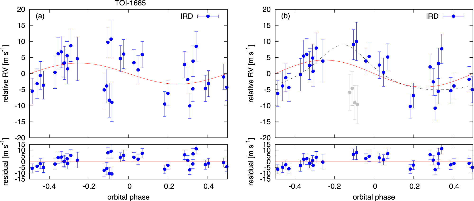
Figure 21. ESM and TSM (Kempton et al. 2018) are plotted for all transiting planets (Rp <2.0 R⊕) with measured masses. Those metrics indicate the relative signals of atmospheric characterizations by emission (ESM) and transmission spectroscopies (TSM). The size of the symbols corresponds to the planet radius.
Download figure:
Standard image High-resolution image
5. Summary
With a goal of confirming and characterizing the USP planet candidates around TOI-1634 and TOI-1685, we conducted intensive follow-up observations for the two targets including ground-based transit photometry, high-resolution imaging, reconnaissance spectroscopy, and high-precision RV measurements. The light curves from the ground-based photometry indicated transit depths consistent with those by the TESS photometry. The ground-based photometry also helped us to refine the orbital periods by more than an order of magnitude compared with the ephemeris obtained from TESS photometry alone. Spectroscopic follow-up observations revealed that the two stars are both ≈M3 dwarfs on the main sequence, having very similar effective temperatures, masses, and radii.
TOI-1634 has a bound, low-mass companion star separated by 25, which is estimated to have ≈0.1 M⊙, whose flux is contaminated in the light curves by both TESS and ground-based photometric observations, but we confirmed that the USP planet is indeed orbiting the primary star through the RV measurements using Subaru/IRD; the periodogram for the RV data exhibits the highest peak at the period of TOI-1634b (0.989 days), and its observed variations indicated the USP planet has a mass of Mp
= 10.14 ± 0.95 M⊕ when a circular orbit is assumed.
On the other hand, TOI-1685's RV data show a more puzzling behavior, but a significant peak (FAP<0.1%) is detected at the right transit period (0.669 days) in the periodogram when the RV points taken during a significant instrumental instability (Feb-02) were removed from the analysis. As a result of fitting the observed RVs without the Feb-02 data, we obtained the USP planet mass of 3.43 ± 0.93 M⊕ for the case of a circular orbit. The residual RVs around the best-fit circular model show an excess scatter, suggesting the presence of a moderate eccentricity, an unknown systematic effect by instrumental or stellar-activity induced noise, and/or an additional planet in the system; the secondary-planet scenario is the most preferred scenario according to the BIC values for different scenarios. The additional periodogram analysis on the residual RVs indeed suggests a possible periodicity at ≈2.6 days, but we were unable to claim that it is an additional planet signal due to the lack of phase coverage and unknown nature of stellar activity. Further observations are needed to confirm the presence of the additional planet(s).
When the planet masses for the circular, one-planet model are adopted (Table 2), both TOI-1634b and TOI-1685b are plotted near the theoretical curve for an Earth-like composition in the MR diagram. Therefore, the two new USP planets should have similar properties to those of all the other USP planets with Rp <3 R⊕, including their internal structure and atmosphere. TOI-1634b is one of the largest and most massive USP planets having an Earth-like composition, and therefore, it would become a benchmark target to study the formation and evolution history of massive USP planets. Both planets are listed among the best suitable targets for future atmospheric studies of small rocky planets by emission spectroscopy thanks to the brightness of the host stars, which encourages future characterizations using large-aperture telescopes including JWST. Although small USP planets (<2 R⊕) are likely to have lost the primordial atmospheres dominated by H2 and He, one may be able to probe and constrain the secondary atmosphere formed via outgassing from the planet interior.
This work is partly supported by JSPS KAKENHI Grant Numbers JP20K14518, JP19K14783, JP18H01265, JP18H05439, JP17H04574, JP18H05442, JP15H02063, JP21H00035, and JP22000005; JST PRESTO grant No. JPMJPR1775; Grant-in-Aid for JSPS Fellows, grant No. JP20J21872; and a University Research Support Grant from the National Astronomical Observatory of Japan (NAOJ). J.N.W. thanks the Heising-Simons Foundation for support. The data analysis was carried out, in part, on the Multi-wavelength Data Analysis System operated by the Astronomy Data Center (ADC), National Astronomical Observatory of Japan.
Based on observations obtained at the Observatoire du Mont-Mégantic, financed by Université de Montréal, Université Laval, the National Sciences and Engineering Council of Canada (NSERC), the Fonds québécois de la recherche sur la Nature et les technologies (FQRNT), and the Canada Economic Development program and the Quebec Ministère de l'Économie et de l'Innovation.
This paper includes data collected by the TESS mission. Funding for the TESS mission is provided by the NASA Explorer Program. We acknowledge the use of TESS Alert data, which is currently in a beta test phase, from pipelines at the TESS Science Office and at the TESS Science Processing Operations Center. Resources supporting this work were provided by the NASA High-End Computing (HEC) Program through the NASA Advanced Supercomputing (NAS) Division at Ames Research Center for the production of the SPOC data products. This research has made use of the Exoplanet Follow-up Observation Program website, which is operated by the California Institute of Technology, under contract with the National Aeronautics and Space Administration under the Exoplanet Exploration Program.
This work has made use of data from the European Space Agency (ESA) mission Gaia (https://www.cosmos.esa.int/gaia), processed by the Gaia Data Processing and Analysis Consortium (DPAC, https://www.cosmos.esa.int/web/gaia/dpac/consortium). Funding for the DPAC has been provided by national institutions, in particular the institutions participating in the Gaia Multilateral Agreement.
This work was enabled by observations made from the Subaru, Gemini North, and Keck telescopes, located within the Maunakea Science Reserve and adjacent to the summit of Maunakea. We are grateful for the privilege of observing the universe from a place that is unique in both its astronomical quality and its cultural significance.
Some of the Observations in the paper made use of the High-Resolution Imaging instrument 'Alopeke. 'Alopeke was funded by the NASA Exoplanet Exploration Program and built at the NASA Ames Research Center by Steve B. Howell, Nic Scott, Elliott P. Horch, and Emmett Quigley. Data were reduced using a software pipeline originally written by Elliott Horch and Mark Everett. 'Alopeke was mounted on the Gemini North telescope of the international Gemini Observatory, a program of NSF's OIR Lab, which is managed by the Association of Universities for Research in Astronomy (AURA) under a cooperative agreement with the National Science Foundation on behalf of the Gemini partnership: the National Science Foundation (United States), National Research Council (Canada), Agencia Nacional de Investigación y Desarrollo (Chile), Ministerio de Ciencia, Tecnología e Innovación (Argentina), Ministério da Ciência, Tecnologia, Inovações e Comunicações (Brazil), and Korea Astronomy and Space Science Institute (Republic of Korea). Data collected under program GN-2020B-LP-105.
This paper is based on observations made with the MuSCAT2 instrument, developed by the Astrobiology Center, at Telescopio Carlos Sánchez operated on the island of Tenerife by the IAC in the Spanish Observatorio del Teide. This paper is based on observations made with the MuSCAT3 instrument, developed by the Astrobiology Center and under financial supports by JSPS KAKENHI (JP18H05439) and JST PRESTO (JPMJPR1775), at Faulkes Telescope North on Maui, HI, operated by the Las Cumbres Observatory.
This work makes use of observations from the LCOGT network. Part of the LCOGT telescope time was granted by NOIRLab through the Mid-Scale Innovations Program (MSIP). MSIP is funded by NSF.
We express special thanks to the anonymous referee for the helpful comments and suggestions on this manuscript.
Facilities: Subaru (IRD) - , Gemini:Gillett ('Alopeke) - , Keck:II (NIRC2) - , LCOGT - , Okayama:1.88m(MuSCAT) - , Sanchez(MuSCAT2) - , FTN (MuSCAT3). -
Software: AstroImageJ (Collins et al. 2017), IRAF (Tody 1993), SpecMatch-Emp (Yee et al. 2017), BANYAN Σ (Gagné et al. 2018), TAPIR (Jensen 2013).
Cloutier et al. (2021) and Bluhm et al. (2021) independently validated and confirmed TOI-1634b and TOI-1685b, respectively, based on their own transit light-curve analyses (both TESS and ground-based ones) and follow-up RV measurements. For both planets, their measured masses (4.91+0.68 -0.70 M⊕ for TOI-1634b and 3.78 ± 0.63 M⊕ for TOI-1685b) were significantly lower than our results, presented in this paper. The reason for the disagreements is unknown, and future observations, preferably using a third spectrograph for RV measurements, would be able to settle the issue.
Footnotes
- *
Based on data collected at Subaru Telescope, which is operated by the National Astronomical Observatory of Japan.
- 45
- 46
- 47
- 48
- 49
Because we defocused the images to achieve a better photometric precision, we are unable to distinguish the fluxes from the two stars.
- 50
In most cases, the instrumental RV drift of IRD is less than 10–20 m s−1 over a few hours, but that night it showed a particularly drastic RV variation during the first half of the night.
- 51