


Abstract
Voyager 2 (V2) crossed the heliopause at 119.0 au on 2018 day 309, after which it observed compressive (longitudinal) magnetic field fluctuations along the average magnetic field direction in the very local interstellar medium (VLISM) at distances from 119.00 to 121.48 au and latitudes 32 2 to 324 S in heliographic inertial coordinates from 2018 day 309 to 2019 day 230. This result confirms the observations of longitudinal magnetic field fluctuations by Voyager 1 (V1) between 124.14 and 128.71 au at 346N (∼2–7 au upwind of the heliopause) from 2013 day 133 to 2014 day 235. V1 crossed the heliopause at 121.58 au and 345N on 2012 day 238. It came as a surprise to find it seemed that V1 observed transverse (Alfvénic) fluctuations of B between 131.40 and 135.98 au at latitude 346–347N (∼10–14 au upwind of the heliopause) from 2015 day 145 to 2016 day 248. The most recent V1 observations show the possible presence of transverse fluctuations of B in the VLISM from 141.44 to 146.01 au at 347–348N (∼20–24 au from the heliopause) between 2018 day 75 and 2019 day 178. Together, these observations show that longitudinal (compressive) magnetic field fluctuations are transmitted through the heliopause from the heliosheath into the VLISM, and are then converted into transverse (Alfvénic) fluctuations at ∼130 au (∼8 au from the heliopause) that are observed out at 146 au (∼24 au from the heliopause).
Export citation and abstract BibTeX RIS
1. Introduction
Voyager 1 (V1) crossed the heliopause on 2012 August 25 (2012.65, day 238) at a distance of 121.58 au from the Sun, and it entered the very local interstellar medium (VLISM) in the northern hemisphere (Burlaga et al. 2013; Gurnett et al. 2013; Krimigis et al. 2013; and Stone et al. 2013). Zank (2015) and Zank et al. (2017, p. 1) defined the VLISM as "that region of the interstellar medium surrounding the Sun that is modified or mediated by heliospheric processes or material." For general overviews of the interaction between the heliosphere and the interstellar medium, see Zank (1999, 2015).
An overview of the magnetic field in the heliosheath is given by Burlaga & Ness (2015). On scales less than 25 days, the turbulence cannot be simply described by a power-law spectrum, but rather has a multifractal structure on scales less than 25 days. Such a structure is appropriate for a driven open nonequilibrium system, and it can be described by the methods of nonextensive statistical mechanics (Burlaga & Viñas 2005; Tsallis 2009). Relatively high levels of compressible turbulence have been observed throughout the heliosheath, e.g., by Burlaga et al. (2006), Burlaga & Ness (2015), and Fraternale et al. (2019). In the distant heliosheath, near the heliopause, Burlaga et al. (2014) examined fluctuations of the hourly averages of the magnetic field B observed by V1 from 2011.0 to 2012.31, where the average magnetic field strength B was 0.17 nT. They found that the fluctuations in the heliosheath were again primarily longitudinal (compressive) fluctuations, varying nearly along the average direction of B.
In the VLISM, Burlaga et al. (2014) examined magnetic field fluctuations, again using hourly averages, observed by V1 during the interval from 2012.6503 to 2013.5855, when the average magnetic field strength B was 0.47 nT. In this case they could not determine whether fluctuations of hourly averages of B were compressive or transverse, because the magnetic field measurements were at the instrument noise level. Burlaga et al. (2014) considered the possibility that the fluctuations in B in the VLISM originated in the heliosheath, but they could not demonstrate that this was the case with the available data.
Burlaga et al. (2015) measured the fluctuations of the magnetic field in the VLISM on a larger scale, using filtered daily averages of the V1 data. In this case they were able to show that the fluctuations were predominantly longitudinal (compressible) in the region ∼2–7 au upwind of the heliopause during a quiet interval from 2013 day 133 to 2014 day 235, between 124.14 au and 128.71 au at 346N, which they called "Interval 1." They also demonstrated that the spectrum of the fluctuations was a Kolmogorov k−5/3 spectrum.
Zank et al. (2017) showed that only compressible fast magnetosonic modes can be transmitted from the inner heliosheath, across the heliopause, and into the VLISM and that they exhibit a k−5/3 spectrum. In particular, they showed that neither Alfvén waves nor slow magnetosonic modes can be transmitted from the inner heliosheath into the VLISM. This result has been confirmed by Matsukiyo et al. (2020) using particle-in-cell (PIC) simulations.
Burlaga et al. (2018) subsequently studied daily averages of magnetic fluctuations in the VLISM observed by V1 during a later quiet interval, "Interval 2," in the region ∼10–14 au upwind of the heliopause between 2015 day 145 and 2016 day 248, at distances between 131.40 and 135.98 au at latitude 346–347N. Surprisingly, they found that in this region the fluctuations were incompressible and dominated by transverse fluctuations of B over the same frequency range. Interval 2 was farther from the heliopause (located at ∼121.6 au) than was Interval 1. Thus, Burlaga et al. (2018) suggested that the nature of the magnetic fluctuations in the VLISM changed, from predominantly longitudinal to predominantly transverse, while moving from 2 to 7 au away from the heliopause to ∼10–14 au.
Since the observations of the fluctuations were contaminated by noise, the authors urged caution and recommended that these observations be confirmed. Fraternale et al. (2019), using the same data but a different method, confirmed that the fluctuations were predominantly transverse during Interval 2. This paper confirms the existence of this transformation of the nature of the fluctuations by studying fluctuations observed by the recent V2 observations near the heliopause (Section 2) and the recent V1 observations made relatively far from the heliopause (Section 3).
Zank et al. (2019) proposed a mechanism to explain the observations of the transformation of the nature of the fluctuations from only predominantly magnetosonic (longitudinal) fluctuations to predominantly Alfvénic (transverse) fluctuations. In particular, they showed theoretically that a low-plasma β VLISM admits three-wave interactions between a fast magnetosonic mode, a zero-frequency mode (an Elsässer vortex), and an Alfvén wave. The fast magnetosonic mode is converted to an incompressible Alfvén mode (or a zero-frequency mode) with wavenumber almost identical to that of the initial compressible fast mode. Fast magnetosonic waves undergo mode conversion via a three-wave interaction as they propagate in the approximately homogeneous VLISM, decaying into an Alfvén wave and a zero-frequency Elsässer vortex, both of which possess only a transverse magnetic field component for the wavelength range observed by V1. Zank et al. (2019) estimated that compressible fast modes are fully mode converted to incompressible fluctuations within ∼10 au of the heliopause, consistent with the observations.
Section 2 of this paper presents V2 observations of the fluctuations of B made just after it crossed the heliopause as V2 began to move through the VLISM. Based on the early results discussed above, we expect to observe longitudinal fluctuations during this interval, because V2 was close to the heliopause, and therefore presumably measuring fluctuations that crossed from the heliosheath into the VLISM, in accordance with the theory of Zank et al. (2019). We shall show that these observations confirm the results of Burlaga et al. (2015) and add additional support for the theory of Zank et al. (2019).
Section 3 of this paper presents the most recent V1 observations of the magnetic field fluctuations, in a third interval, Interval 3, between 2018 day 75 and 2019 day 178 from 141.44 to 146.01 au at ∼35°N. It will be shown that these observations in the VLISM even farther from the heliopause are still transverse observations. This result is further evidence that the fluctuations in the VLISM are fundamentally different than those observed in the heliosheath. Finally, we discuss and summarize the findings in Section 4.
2. Voyager 2 Observations of the VLISM Magnetic Field and its Fluctuations
The aim of this part of the paper is to describe the variations in the magnetic field observed recently by V2 in the region of the VLISM that was adjacent to the heliopause, which was crossed on 2018 day 309 and extends to 2019 day 230 at distances from 119.00 to 121.48 au at ∼323S, which is the current limit of the available V2 magnetic field observations. The crossing of the heliopause was predicted by Washimi et al. (2017).
Figure 1 shows daily averages of the magnetic field observations made by V2 during 2018 and 2019. V2 crossed the heliopause on 2018 day 309 (November 5), which is shown by the vertical solid line in Figure 1. A distinguishing feature of the heliopause in Figure 1 is the large increase in the magnetic field strength to 0.7 nT when V2 began to observe the magnetic field of the VLISM, compared to 0.44 nT observed earlier at heliopause by V1. Additional observations identifying and describing the heliopause crossing by V2 and its neighboring regions were discussed by Burlaga et al. (2019a), Krimigis et al. (2019), Richardson et al. (2019), and Stone et al. (2019). During the interval from 2018 day 309 to 2019 day 230, in Figure 1, the average azimuthal and elevation angles of B,  and
and  , were 267° ± 3° and 243 ± 04, respectively. These angles are close to the Parker spiral magnetic field direction,
  and
and  (Parker 1971a, 1971b), which is surprising since there is no reason for the direction of the magnetic field in the VLISM to be along the spiral magnetic field direction.
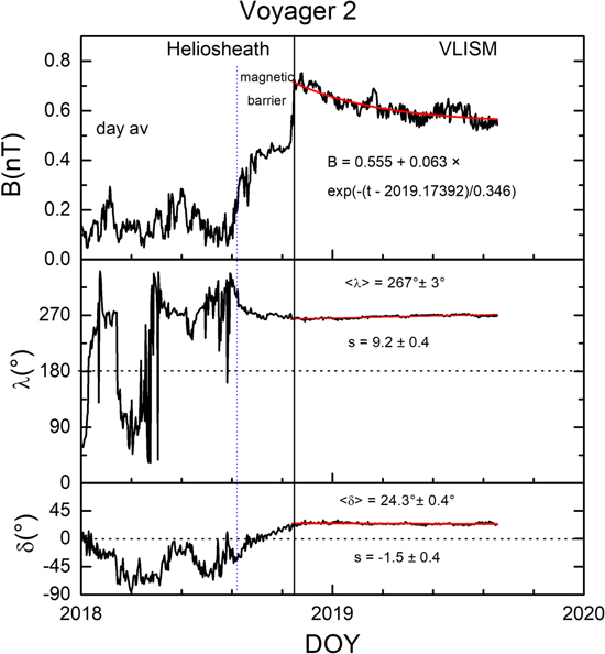
Figure 1. (a) Daily averages of magnetic field strength B, (b) the azimuthal angle λ, and (c) the elevation angle δ, observed by V2 from the time it crossed the heliopause (hp) into the VLISM on 2018.84587 at 119.0 au to 2019.63014 at 121.48 au. The red curve in the top panel is an exponential fit to the observations of B(t), which might be related to outward motion of the heliopause. Linear fits to λ(t) and δ(t) with slope "s" are shown in panels in lower panels (b) and (c), respectively.
Download figure:
Standard image High-resolution imageObservations of the heliosheath prior to the heliopause crossing are shown on the left side of Figure 1. Although the heliosheath and VLISM are very different, they are not independent. Both V1 and V2 observations show that the magnetic field direction did not change across the heliopause. Instead, Figure 1 shows that there was a smooth rotation of the magnetic field direction from the sunward side of the magnetic barrier (Washimi et al. 2011, 2017 Pogorelov et al. 2017) through the heliopause and into the VLISM as discussed by Burlaga et al. (2019a) for the V2 observations and by Burlaga et al. (2014) for the V1 data. It is well established that shocks and even pressure waves observed in the VLISM originate in the heliosphere. And, as we shall demonstrate in this paper, longitudinal fluctuations of the magnetic field can be transmitted from the heliosheath across the heliopause and into the VLISM, as suggested earlier.
Following the heliopause crossing, the magnetic field strength B of the interstellar magnetic field that was draped around the heliosphere decreased exponentially from 0.7 nT at the heliopause as 0.555+0.063 × exp(-(t-2019.17392)/0.346) with an exponential decay time of ∼125 days, and it approached 0.56 nT at the end of the data set shown in Figure 1. It seems possible that the relatively strong field and the exponential decay might be the result of outward motion of the heliopause. The magnetic field in the interstellar medium (ISM) was calculated by Izmodenov et al. (2020) who found, using a model and observations including the Voyager data, that BISM = 3.7–3.8 μG ∼ 0.4 nT directed toward ≈125° in longitude, and ≈37° in latitude in the heliographic inertial coordinate system. Whang (2010) calculated that BISM increased by as much as 1.6 as a result of draping, which would imply that the magnetic field in the VLISM could be as high as 1.6 times the interstellar magnetic field. For BISM ∼ 0.4 nT from Izmodenov & Alexashov (2020), Whang's result implies that the draped interstellar magnetic field as V2 could have been as large as 0.6 nT. The results of Whang (2010) and Izmodenov & Alexashov (2020) are consistent with the V2 observations of 0.7 nT.
As discussed in the introduction, Burlaga et al. (2014, 2015) emphasized the need to confirm the compressive nature of the magnetic field fluctuations observed by V1 near the heliopause with further measurements, since the signal was weak and it was contaminated by noise. The V2 observations allow us to confirm whether the fluctuations in B were compressive, as observed by V1 (Burlaga et al. 2015) and predicted by Zank et al. (2019), as discussed in the following paragraph. The fluctuations (δ B) of the measured magnetic field strength B and the components of B, in the spacecraft centered RTN coordinate system (in which the dimensionless unit vector R is directed radially away from the sun, T is parallel to the solar equatorial plane and aligned with the direction of the sun's rotation, and the unit vector N completes the right-handed coordinate system), were obtained by subtracting the large-scale exponential trend from the observations of B and the components of B from 2018 day 309 to 2019 day 230. As shown in Figure 2, the magnetic field strength B and the magnitude of the BR, BT, and BN components decreased exponentially with increasing time and increasing distance from the heliopause. The BT component was the largest component, comparable to B. The BR component was the smallest component, decreasing from less than 0.1 nT near the heliopause to ∼0 nT beyond 2019.4.

Figure 2. Daily averages of the V2 magnetic field strength B, the components BN, BR, and BT, respectively, in the spacecraft centered RTN coordinate system as a function of time. The smooth curves are exponential fits to these quantities.
Download figure:
Standard image High-resolution imageFigure 3 shows the fluctuations of the magnetic field components and strength as a function of time that were measured by V2 from 2018 day 309 to 2019 day 230 between 119.00 and 121.48 au. Near the heliopause, the fluctuations in the BR(t) component and the BN(t) component (δBR(t) and δBN(t), respectively) in panels b and d of Figure 3 are significantly smaller than the fluctuations δB(t) and δBT(t) in panel a and panel c, respectively. This result is confirmed by the values of the standard deviations (SDs) of the fluctuations, which were 0.013 nT for δBR(t) and 0.016 nT for δBN(t). The δBR and δBN were approximately half as large as δBT (0.027 nT), which is comparable to the value 0.029 nT of the SD for δB. In other words, the fluctuations in δBT were comparable to those in δB, and they were significantly larger than the fluctuations in δBR and δBN.
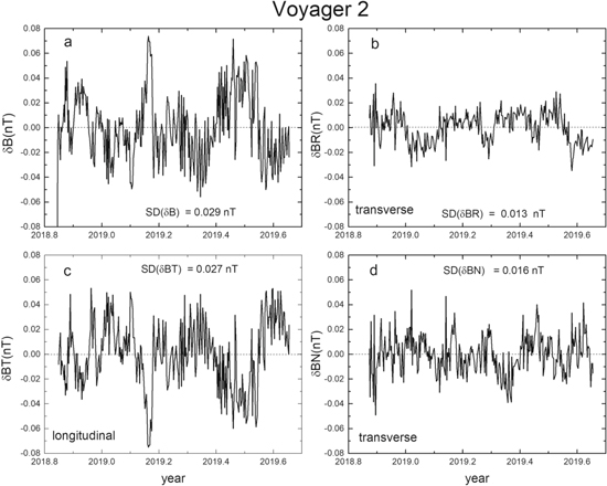
Figure 3. (a)–(d) Fluctuations of daily averages of (a) the detrended magnetic field strength, (b) δBR, (c) δBT, and (d) δBN measured by V2 as a function of time. The smallest fluctuations were in δBR and δBN as indicated by the SDs. The largest fluctuations were in the BT components of B, δBT, which were comparable in magnitude to the fluctuations in δB, indicating that they are longitudinal fluctuations.
Download figure:
Standard image High-resolution imageThe direction of the normalized average magnetic field was  R–0.91 T + 0.41 N, where the average magnetic field strength was Bav = 0.62 nT. Since the normalized average magnetic field direction is close to the BT direction (BT/Bav = −0.919), the fluctuations were primarily along the average magnetic field. Hence, the fluctuations were primarily longitudinal (compressive, perhaps magnetosonic) fluctuations. Since the T direction has coordinates λ = 270° and δ = 0°, the T direction was nearly along the normalized average magnetic field direction
  , for which λ = 267° ± 3° and δ = 243 ± 04. Specifically, the angle between
  and T was cos−1
  . Thus, the fluctuations in B were primarily along the average magnetic field direction. We conclude that the magnetic field fluctuations observed by V2 in the VLISM adjacent the heliopause were primarily longitudinal fluctuations.
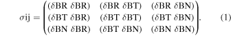
The preceding analysis is based directly on the measurements made by the magnetometers on V2. A more refined analysis, which is less direct, is based on the maximum variance method which gives the eigenvectors of B and the corresponding eigenvalues of the covariance matrix. The 3 × 3 covariance matrix σij can be calculated from the averages of the products of pairs of δBR, δBT, and δBN divided by the number of observations in the matrix
The eigenvectors of this matrix determine the dimensionless minimum variance direction Bm, the intermediate direction Bi, and the maximum variance direction BM. The corresponding eigenvalues obtained using this approach are 10−4 × (0.519, 3.018, 8.262), indicating that there is a clear maximum variance direction and a well-defined minimum variance direction. The corresponding eigenvectors are Bm = (−0.828 R̃ −2.74 T, −0.490 N), Bi = (0.515 R, −0.025 T, −0.857 N), and BM = (−0.222 R, 0.962 T, −0.161 N), respectively. The angle θ between the maximum variance direction BM and the average normalized magnetic field B/Bav in the preceding paragraph is determined by the dot product BM • B/Bav = cos(θ), which gives θ = 31°, and it is consistent with the estimate θ = 24° given above within the uncertainties. Again, we conclude that the fluctuations of the magnetic field B were nearly along the average magnetic field, indicating that they were longitudinal fluctuations, possibly magnetosonic fluctuations.
We also conduct a power spectrum analysis of the fluctuations of the magnetic field measured by V2 from 2018 day 310 to 2019 day 230, as shown in Figure 4. These power spectra are basically consistent with the Kolmogorov k−5/3 spectrum from 8 × 10⁻⁸ to 7 × 10⁻⁷ Hz, except BN. At frequencies higher than 7 × 10⁻⁷ Hz, the slopes of these power spectra are lower than −5/3 for the Kolmogorov turbulence.

Figure 4. (a)–(d) Spectra of the magnetic field fluctuations δBR, δBT, δBN, and δB observed by V2. The dashed line is the Kolmogorov k−5/3 spectrum which shows that the fluctuations in all components except BN tend to follow the Kolmogorov spectrum.
Download figure:
Standard image High-resolution imageIn Figure 5, we compare the compressional power (in blue) and transverse power (in red) of magnetic field fluctuations observed by V2 in the same interval. From 8 × 10⁻⁸ to 7 × 10⁻⁷ Hz, the slope of the transverse power spectrum is nearly consistent with the Kolmogorov k−5/3 spectrum while the slope of the compressional power spectrum is less steep than −5/3. At higher frequency, the slopes of both compressional and transverse power spectral densities are less steep than −5/3, possibly associated with intermittency and noise. This figure clearly shows the dominance of compressional fluctuations relative to transverse fluctuations, as shown by our former analysis of the observed fluctuations of the components of the magnetic field.

Figure 5. Spectra of the transverse power (red) and compressional power (blue) observed by V2. There is an enhancement in the compressional power relative to the transverse power between 2 × 10⁻⁷ Hz and 1.5 × 10⁻⁶ Hz, consistent with our conclusion derived from observational time series that show a dominance of compressional (longitudinal) fluctuations relative to transverse fluctuations.
Download figure:
Standard image High-resolution imageThe above results obtained from the recent V2 observations in the southern hemisphere at latitude 323S are consistent with the earlier results of Burlaga et al. (2015) obtained from V1 observations in the northern hemisphere at 346N. They also found that the fluctuations near but not adjacent to the heliopause (during the Interval 1 in Figure 6 discussed in the next section) were longitudinal fluctuations.
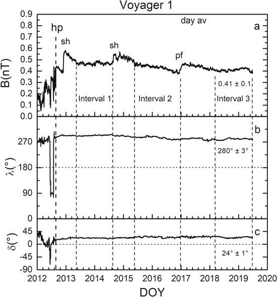
Figure 6. (a) Daily averages of the magnetic field strength B, (b) the azimuthal angle λ, and (c) the elevation angle δ, observed by V1 as a function of time in years. The fluctuations during the relatively undisturbed intervals (Interval 1, Interval 2, and Interval 3) are discussed in the text. These intervals were not close to the principal disturbances, namely the two shocks (sh) and the pressure front (pf).
Download figure:
Standard image High-resolution imageThese results strongly support the hypothesis of Burlaga et al. (2014) that the longitudinal (compressive) magnetic fluctuations from the heliosheath can cross the heliopause and be observed in the VLISM near the heliopause. The theory of Zank et al. (2017) shows that only compressive fluctuations from the heliosheath can cross the heliopause and enter the VLISM.
3. Voyager 1 Observations of the VLISM Magnetic Field and its Fluctuations
V1 crossed the heliopause into the VLISM on 2012 day 238 at 121.58 au (Burlaga et al. 2013; Gurnett et al. 2013; Krimigis et al. 2013; Stone et al. 2013) and it has remained in the VLISM until at least 2019.49 (2019 day 178). All of the daily averages of the magnetic field strength and direction in the VLISM are plotted in Figure 6. The latest observations, that are the subject of this paper, are the 2018–2019 data.
Several notable features in the earlier V1 VLISM data shown in Figure 6 were discussed previously. There were two shocks (labeled sh) characterized by a significant increase in B during 2012 (Burlaga & Ness 2014; Burlaga & Ness 2016). In each case, the magnetic field strength decreased following an outward propagating shock during a significant fraction of a year. A third notable increase in B, which was too broad to be a shock, was identified as a pressure front (labeled pf; Burlaga et al. 2019b). It was observed at the beginning of 2017, and followed by decreasing magnetic field strength for approximately one year. Each of the shocks and associated strong magnetic fields was followed by an extended interval with weaker and nearly uniform magnetic fields, labeled Interval 1 and Interval 2, respectively in Figure 6. The pressure front and its decaying magnetic field strength were followed by another interval with relatively weak and uniform magnetic fields, Interval 3, in the latest data, which is the main subject of this section.
We take the beginning of Interval 3 to be 2018.20469 (2018 day 75) and the end of the interval as the end of the data set on 2019.48629 (2019 day 178). Figure 7 shows the magnetic field strength B and the components BR, BT, and BN as a function of time during this interval. The uncertainties in these components is discussed by Berdichevsky (2009), and the instrument is described by Behannon et al. (1977). A linear least-squares fit was made to the data for B and each of its components, which is shown by the straight red lines in Figure 7. A linear trend is apparent for each of the components and for B. The slopes of the straight lines obtained from the fit are (0.011 ± 0.001) nT yr−1 for B, (0.016 ± 0.005) nT yr−1 for BN, (0.023 ± 0.002) nT yr−1 for BR, and (−0.006 ± 0.001) nT yr−1 for BT. All of the slopes of the linear fits are statistically significant, but higher-order polynomial fits are not justified.
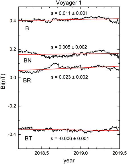
Figure 7. Daily averages of the V1 magnetic field strength B, and the components BN, BR, and BT, respectively, in the spacecraft centered RTN coordinate system as a function of time. The smooth lines are linear fits to these quantities with slopes "s."
Download figure:
Standard image High-resolution imageSubtracting the linear fits from the observations of B, BR, BT, and BN gives the fluctuations of the respective quantities that are plotted in Figure 8. The curves for δB ≡ (B − Bfit)(t) and δBT ≡ (BT − BTfit)(t) in Figures 8(a) and (c), respectively, are very similar, except for the sign. In particular, the SD is 0.011 nT for both curves, which is very small, close to the electronic noise level of the instruments, 0.005 nT. On the other hand, the curves for δBR ≡ (BR − BRfit)(t) and δBN ≡ (BN − BNfit)(t) in Figures 8(b) and (d), respectively, are somewhat different. The curve in Figure 8(b) is more disordered than that in Figure 8(d) which happens to be nearly sinusoidal. Nevertheless, both curves have the same standard deviation, 0.015 nT, which is significantly larger than that for the curves in Figures 6(a) and (c), although the fluctuations are small and contaminated by noise.
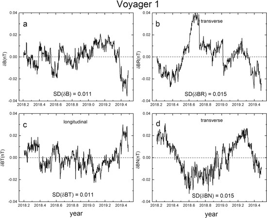
Figure 8. (a)–(d) Fluctuations of daily averages of (a) the detrended magnetic field strength δB, (b) δBR, (c) δBT, and (d) δBN measured by V1 as a function of time. The smallest fluctuations were in δBT and δB indicated by the SDs. The largest fluctuations were in δBR and δBN, which were comparable in magnitude, having the same standard deviations SDs. These fluctuations were orthogonal to the average magnetic field direction, thus they were transverse fluctuations.
Download figure:
Standard image High-resolution imageFor the V1 observations in Interval 3 shown in Figure 6, the magnitude of the average magnetic field  was B = 0.410 nT. The unit vector in the direction of the average magnetic field was
  . Thus, the results of the previous paragraph and Figure 8 suggest that the largest fluctuations were in the R–N plane, which was perpendicular to the average magnetic field direction. Thus, the fluctuations observed by V1 were primarily transverse fluctuations.
Using the minimum variance approach discussed in Section 2, the eigenvectors of the covariance matrix determine the minimum variance direction Bm, the intermediate direction Bi, and the maximum variance direction BM. The corresponding eigenvalues obtained using this approach are 10−4 × (0.726, 1.495, 3.100), indicating that there was a clear maximum variance direction and minimum variance direction. The corresponding eigenvectors are Bm = (0.395 R, 0.893 T, 0.216 N), Bi = (−0.578 R, 0.424 T, −0.697 N), and BM = (−0.714 R, 0.151 T, 0.635 N), respectively. The angle θ between the maximum variance direction BM and the average normalized magnetic field B/Bav given in the previous paragraph is determined by the dot product BM • B/Bav = 0.01 = cos(θ), which gives θ = 90°. We conclude that the fluctuations of the magnetic field B were nearly transverse to the average magnetic field, indicating that the fluctuations were primarily transverse fluctuations, presumably Alfvénic fluctuations.
The above results, obtained from the recent V1 observations during Interval 3 in the northern hemisphere from 141.44 to 146.01 au at latitude ∼347N, are consistent with the earlier results of Burlaga et al. (2018) which were obtained from V1 observations during Interval 2 in the northern hemisphere at ∼346N. They also found that the fluctuations moderately far from the heliopause at 131.40 to 135.98 au, during the Interval 2 in Figure 6, were transverse fluctuations. These results support the observation of Burlaga et al. (2018) that the longitudinal (compressive) magnetic fluctuations near the heliopause in the VLISM can be converted to transverse fluctuations farther from the heliopause. The theory of Zank et al. (2019) predicts that longitudinal fluctuations of the magnetic field near the heliopause can be converted to transverse fluctuations farther from the heliopause, as confirmed by the data in this paper.
We also conduct a power spectrum analysis of the fluctuations of the magnetic field measured by V1 in Interval 3 as shown in Figure 9. These power spectra are basically consistent with the Kolmogorov k−5/3 spectrum from 5 × 10⁻⁸ to 8 × 10⁻⁷ Hz. At frequencies higher than 8 × 10⁻⁷ Hz, the slopes of these power spectra are lower than −5/3 for the Kolmogorov turbulence.

Figure 9. (a)–(d) Spectra of the magnetic field fluctuations δBR, δBT, δBN, and δB observed by V1. The dashed line is the Kolmogorov spectrum which shows that the fluctuations in all components in VLISM tend to follow the Kolmogorov spectrum.
Download figure:
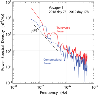
Standard image High-resolution imageIn Figure 10, we compare the compressional power (in blue) and transverse power (in red) of magnetic field fluctuations observed by V1 in the same interval. From 5 × 10⁻⁸ to 8 × 10⁻⁷ Hz, the slope of the compressional power spectrum is nearly consistent with the Kolmogorov  spectrum while the slope of the transverse power spectrum is steeper than −5/3. At higher frequency, the slopes of both compressional and transverse power spectral densities are less steep than −5/3, possibly associated with intermittency and noise. This figure clearly shows the dominance of transverse fluctuations relative to compressional fluctuations as far as 146 au, as shown by our analysis of the observed magnetic field fluctuations far from the Sun.
Figure 10. Spectra of the transverse power (red) and compressional power (blue) observed by V1. There is an enhancement in the transverse power relative to the compressional power between 2 × 10⁻⁷ Hz and 10−6 Hz, consistent with our conclusion derived from observational time series that show a dominance of transverse fluctuations relative to compressional (longitudinal) fluctuations.
Download figure:
Standard image High-resolution image
4. Summary and Discussion
This paper discusses the most recent observations of magnetic field fluctuations by V2 at distances from 119.00 to 121.48 au which crossed the heliopause at 119.0 au on 2018 day 309, as well as the most recent observations of magnetic field fluctuations by V1 from 141.44 to 146.01 au at ∼35°N in the VLISM in the context of earlier V1 observations in the VLISM with the aim of understanding the nature and behavior of these fluctuations.
We find that V2 in the southern hemisphere at ∼32°S observed longitudinal (compressive) fluctuations in the magnetic field along the average magnetic field direction B from the time that V2 crossed the heliopause at 119.00 au to 121.48 au, which corresponds to the end of the available data set. V1 crossed the heliopause at 121.58 au and entered the VLISM on 2012 day 238, at 345 N. In this case a shock was observed at 122.53 au on 2012 ∼day 335. Therefore, the data for the relatively undisturbed interval from 2013 day 133 to 2014 day 235 (from 124.14 to 128.71 au) were selected for analysis of the fluctuations. The exact distance to the heliopause at these times is not known, because the heliopause might have been moving, but the distance to the heliopause was of the order of 2.5 to 7 au. In this case, V1 again observed compressive fluctuations near the heliopause in the VLISM. Burlaga et al. (2014) suggested that longitudinal fluctuations observed in the heliosheath might be transmitted across the heliopause from the heliosheath and into the VLISM, but there was no definitive observational evidence for this at the time.
A surprising result, reported by Burlaga et al. (2018), showed that V1 observed transverse fluctuations B between 131.40 and 135.98 au at latitude 346N (∼10–14 au upwind of the heliopause) from 2015 day 145 to 2016 day 248, although the fluctuations were significantly contaminated by noise. The most recent V1 observations show the continued presence of transverse fluctuations of B in the VLISM from 141.44 to 146.01 au at 347N (∼20–24 au from the heliopause) between 2018 day 75 and 2019 day 178, again significantly contaminated by noise. Thus, we find that beyond ∼10 au from the heliopause the magnetic fields in the VLISM are likely predominantly transverse fluctuations, that are present throughout the VLISM out to at least 146 au and perhaps well beyond. Thus, the fluctuations in the VLISM may be predominantly Alfvénic.
Together, these observations indicate that longitudinal (compressive) magnetic field fluctuations are transmitted through the heliopause from the heliosheath into the VLISM, but shortly thereafter they are converted into transverse (Alfvénic) fluctuations at ∼131 au (∼10 au from the heliopause) which persist out to at least 146 au (∼24 au from the heliopause). Indeed, Zank et al. (2019) showed that the compressive magnetic fluctuations can be converted to transverse magnetic fluctuations by a mode conversion process, which they discussed in their paper. In other words, beyond ∼10 au from the heliopause the magnetic fluctuations in the VLISM are transverse fluctuations. This in turn implies that compressive fluctuations are not characteristic of the VLISM, except near the heliopause. From this, we conclude that the compressive fluctuations observed in the VLISM near the heliopause were produced by compressive fluctuations in the heliosheath that were transmitted across the heliopause and persisted for at least a short distance of the order of 10 au, before the mode conversion into transverse fluctuations of B. Future V1 observations will show whether or not the dominance of the transverse fluctuations of B will continue to be observed, and future V2 observations will confirm whether the transverse fluctuations replace the dominance of compressive fluctuations as it travels further away from the heliopause.
J.P. was supported by the NASA Voyager Project to the NASA/GSFC Magnetometer Team under internal NASA funding. N.F.N. was supported by the NASA Voyager Project under a cooperative agreement to the University of Maryland, Baltimore County. L.F.B. was supported by the NASA contract 80GSFC19C0012. D.B.B. was supported by the Voyager Project under a cooperative agreement with the TRIDENT-BERTICHEVSKY DANIEL B. partnership. J.K.L thanks the support from NASA's Living with a Star and Heliophysics Supporting Research programs. We thank OMNIWeb of Space Physics Data Facility (https://omniweb.gsfc.nasa.gov/coho/helios/heli.html) for providing the spacecraft orbit data to public.