


Abstract
We report the discovery by the HATSouth project of five new transiting hot Jupiters (HATS-54b through HATS-58Ab). HATS-54b, HATS-55b, and HATS-58Ab are prototypical short-period (P = 2.5–4.2 days, Rp ∼ 1.1–1.2  ) hot Jupiters that span effective temperatures from 1350 to 1750 K, putting them in the proposed region of maximum radius inflation efficiency. The HATS-58 system is composed of two stars, HATS-58A and HATS-58B, which are detected thanks to Gaia DR2 data and which we account for in the joint modeling of the available data—with this, we are led to conclude that the hot Jupiter orbits the brighter HATS-58A star. HATS-57b is a short-period (2.35 day), massive (3.15
  ), 1.14
  , dense (
 ) hot Jupiter orbiting a very active star (2% peak-to-peak flux variability). Finally, HATS-56b is a short-period (4.32 day), highly inflated hot Jupiter (1.7
  , 0.6
, 0.6  ), which is an excellent target for future atmospheric follow-up, especially considering the relatively bright nature (V = 11.6) of its F dwarf host star. This latter exoplanet has another very interesting feature: the radial velocities show a significant quadratic trend. If we interpret this quadratic trend as arising from the pull of an additional planet in the system, we obtain a period of
  days for the possible planet HATS-56c, and a minimum mass of
 . The candidate planet HATS-56c would have a zero-albedo equilibrium temperature of Teq = 332 ± 50 K, and thus would be orbiting close to the habitable zone of HATS-56. Further radial-velocity follow-up, especially over the next two years, is needed to confirm the nature of HATS-56c.
Export citation and abstract BibTeX RIS
1. Introduction
With more than 3000 confirmed exoplanets,20 the field of exoplanet discovery and characterization has seen an exponential increase in the number of discovered far-away worlds. While space-based dedicated surveys such as Kepler (Borucki et al. 2010) have excelled at the detection of small (Rp < 4R⊕) exoplanets, ground-based dedicated surveys such as HATNet (Bakos et al. 2004), HATSouth (Bakos et al. 2013), WASP (Pollacco et al. 2006), KELT (Pepper et al. 2018), and the recently started MASCARA (Snellen et al. 2012) and NGTS (Wheatley et al. 2018) surveys have been pioneering the search of giant exoplanets. This has produced a sample of exoplanets amenable for characterization both in terms of radial-velocity (RV) follow-up—which allows us to constrain their densities—or in terms of atmospheric follow-up—which allows us to have a glimpse at what their atmospheres look like. It has also generated a large sample of well-characterized exoplanets from which we have been able to extract useful information to put our planet formation and evolution theories to test.
Despite the relatively large number of known exoplanets, less than 10% (∼300) are well characterized (i.e., have a mass and radius constrained to better than 20% precision). Discovered mostly from ground-based transit surveys, these often-short-period (P ≲ 10 days) and hot transiting giant exoplanets have provided unique information that has aided the understanding of the formation, evolution, and composition of those far-away worlds. For example, structure modeling coupled with the mass, radius, and ages of the warmer (<1000 K) of these systems has allowed us to understand that they are heavily enriched in metals (Thorngren et al. 2016), which in turn has explicit predictions for their compositions (Espinoza et al. 2017). This understanding, in turn, has allowed us to calibrate how mass and heavy elements are related, which in turn has been used to elucidate the nature of the observed radius inflation of highly irradiated giant exoplanets, bringing us closer to an understanding of the mechanism(s) producing this radius anomaly over a wide range of stellar irradiation, masses, and sizes (Sestovic et al. 2018; Thorngren & Fortney 2018). In terms of formation, short-period giant exoplanets are fundamental probes of the mechanisms that shape their orbits to their present-day forms. Although in situ formation has still not been ruled out (Batygin et al. 2016), the orbital migration scenario—either by direct disk migration and/or by interaction with other bodies in the system (see, e.g., Lin et al. 1996; Li et al. 2014; Petrovich 2015)—is by far the most popular theory to explain the observed short-period orbits of these hot giant exoplanets. All of them have discernible features that can be studied with transiting exoplanets, for which one is able to unveil their three-dimensional orbital shapes if sufficient follow-up is performed. In addition, some transiting systems actually reside in systems with other planetary or substellar companions (see, e.g., Becker et al. 2015; Rey et al. 2018; Sarkis et al. 2018; Yee et al. 2018), which provide new laboratories to study how multiplanetary systems form and evolve.
In this work, we present the discovery of five new transiting hot giant exoplanets, one of which is in a possible multiplanetary system with a substellar companion on a possible temperate, eccentric orbit. The paper is divided as follows. Section 2 details our observations, including the HATSouth photometric detection and both photometric and RV follow-up. Section 3 details the analysis of the data presented, while in Section 4 we discuss our results. Finally, in Section 5 we present our conclusions.
2. Observations
2.1. Photometric Detection
The photometric detection of the exoplanets presented in this work was made with the HATSouth units based in Las Campanas Observatory (LCO; HS-1 and HS-2), at the HESS site in Namibia (HS-3 and HS-4), and at the site in Siding Spring Observatory (SSO; HS-5 and HS-6), the operations of which are described in detail in Bakos et al. (2013). The details of these observations for each of the presented exoplanets can be found in Table 1.
Table 1. Summary of Photometric Observations
| Instrument/Fielda | Date(s) | No. of Images | Cadenceb | Filter | Precisionc |
|---|---|---|---|---|---|
| (s) | (mmag) | ||||
| HATS-54 | |||||
| HS-2/G700 | 2011 Apr–2012 Jul | 4521 | 292 | r | 9.8 |
| HS-4/G700 | 2011 Jul–2012 Jul | 3799 | 301 | r | 10.4 |
| HS-6/G700 | 2012 Jan–2012 Jul | 1425 | 300 | r | 10.7 |
| Swope 1 m | 2016 Feb 09 | 89 | 79 | i | 2.2 |
| PEST 0.3 m | 2016 Feb 25 | 169 | 132 | RC | 6.3 |
| CHAT 0.7 m | 2017 Feb 12 | 50 | 222 | i | 2.1 |
| LCO 1 m/SAAO/DomeB | 2017 May 10 | 73 | 221 | i | 1.7 |
| Swope 1 m | 2017 May 30 | 137 | 160 | g | 1.9 |
| LCO 1 m/SAAO/DomeC | 2017 Jul 05 | 78 | 221 | i | 2.2 |
| LCO 1 m/SSO/DomeB | 2017 Jul 13 | 68 | 224 | i | 3.1 |
| HATS-55 | |||||
| HS-2/G602 | 2011 Aug–2012 Feb | 4192 | 295 | r | 8.8 |
| HS-4/G602 | 2011 Aug–2012 Feb | 3047 | 296 | r | 9.3 |
| HS-6/G602 | 2011 Oct–2012 Feb | 1248 | 303 | r | 8.8 |
| PEST 0.3 m | 2015 Feb 14 | 171 | 132 | RC | 5.1 |
| PETS 0.3 m | 2015 Mar 03 | 144 | 132 | RC | 4.8 |
| Swope 1 m | 2015 Apr 01 | 250 | 59 | i | 3.1 |
| LCO 1 m/CTIO/DomeA | 2017 Apr 10 | 69 | 220 | i | 1.8 |
| LCO 1 m/CTIO/DomeC | 2017 Apr 10 | 69 | 220 | i | 2.5 |
| HATS-56 | |||||
| HS-4/G698 | 2015 May–2015 Jul | 5 | 499 | r | 4.7 |
| HS-6/G698 | 2015 Dec–2016 Jun | 4846 | 343 | r | 6.6 |
| HS-2/G698 | 2015 Mar–2016 May | 2487 | 352 | r | 4.6 |
| HS-4/G698 | 2015 Mar–2016 Jun | 6851 | 324 | r | 5.6 |
| HS-6/G698 | 2015 Mar–2016 Jun | 5638 | 343 | r | 6.1 |
| PEST 0.3 m | 2017 Mar 05 | 182 | 134 | RC | 2.0 |
| LCO 1 m/CTIO | 2017 Mar 22 | 139 | 130 | i | 1.1 |
| LCO 1 m/SSO | 2017 Mar 27 | 47 | 130 | i | 0.8 |
| HATS-57 | |||||
| HS-1/G548 | 2014 Sep–2015 Feb | 5719 | 287 | r | 11.5 |
| HS-2/G548 | 2014 Jun–2015 Apr | 7689 | 348 | r | 10.4 |
| HS-3/G548 | 2014 Sep–2015 Mar | 5214 | 353 | r | 10.5 |
| HS-4/G548 | 2014 Jun–2015 Mar | 5430 | 352 | r | 10.6 |
| HS-5/G548 | 2014 Sep–2015 Mar | 5041 | 359 | r | 10.6 |
| HS-6/G548 | 2014 Jul–2015 Mar | 5989 | 351 | r | 10.7 |
| CHAT 0.7 m | 2017 Aug 28 | 83 | 143 | i | 1.3 |
| CHAT 0.7 m | 2017 Oct 21 | 90 | 146 | i | 1.6 |
| HATS-58 | |||||
| HS-1/G699 | 2011 Apr–2012 Aug | 3645 | 290 | r | 4.9 |
| HS-3/G699 | 2011 Jul–2012 Aug | 3150 | 291 | r | 5.7 |
| HS-5/G699 | 2011 May–2012 Aug | 750 | 290 | r | 4.7 |
| PEST 0.3 m | 2017 Mar 09 | 220 | 132 | RC | 2.2 |
| PEST 0.3 m | 2017 Apr 20 | 223 | 132 | RC | 2.2 |
| LCO 1 m+SAAO/DomeB | 2017 May 15 | 40 | 130 | i | 0.7 |
| LCO 1 m+SSO/DomeB | 2017 Jul 05 | 106 | 134 | i | 2.6 |
Notes.
aFor HATSouth data, we list the HATSouth unit, CCD, and field name from which the observations are taken. HS-1 and -2 are located at Las Campanas Observatory in Chile, HS-3 and -4 are located at the H.E.S.S. site in Namibia, and HS-5 and -6 are located at Siding Spring Observatory in Australia. Each unit has four CCDs. Each field corresponds to one of 838 fixed pointings used to cover the full 4π celestial sphere. All data from a given HATSouth field and CCD number are reduced together, while detrending through External Parameter Decorrelation (EPD) is done independently for each unique unit+CCD+field combination. bThe median time between consecutive images rounded to the nearest second. Due to factors such as weather, the day–night cycle, guiding, and focus corrections, the cadence is only approximately uniform over short timescales. cThe rms of the residuals from the best-fit model.Download table as: ASCIITypeset image
As with previous results from our group, the data were reduced and analyzed with the procedures detailed in Bakos et al. (2013) and Penev et al. (2013); in brief, the light curves were detrended using the trend-filtering algorithm (Kovács et al. 2005) as described in Bakos et al. (2013), and then a search for periodic, transit-like signals using the box-fitting least-squares algorithm (BLS; see Kovács et al. 2002) was performed. Peaks in the BLS periodogram were found for HATS-54, HATS-55, HATS-56, HATS-57, and HATS-58 with periods of 2.54, 4.20, 4.32, 2.35, and 4.21 days, respectively, which prompted us to obtain further photometric and spectroscopic follow-up in order to confirm the planetary nature of the signals, which we detail in the following sections. The phase-folded light curves for each planet are presented in Figures 1 and 2. The data are described in Table 1 and presented in Table 2.
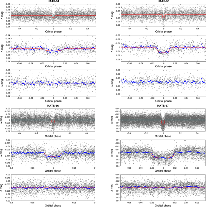
Figure 1. Phase-folded unbinned HATSouth light curves for HATS-54 (upper left), HATS-55 (upper right), HATS-56 (bottom left), and HATS-57 (bottom right). In each case we show three panels. The top panel shows the full light curve, the middle panel shows the light curve zoomed-in on the transit, and the bottom panel shows the residuals from the best-fit model zoomed-in on the transit. The solid lines show the model fits to the light curves. The dark filled circles in the middle and bottom panels show the light curves binned in phase with a bin size of 0.002. The slight systematic discrepancy between the model and binned values in the middle panel is an artifact of plotting data from multiple HATSouth fields for which the effective transit dilution differs. The quality of the fit in this case is best judged by inspection of the residuals shown in the bottom panel.
Download figure:
Standard image High-resolution image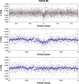
Figure 2. Same as Figure 1, here we show the phase-folded unbinned HATSouth light curves for HATS-58.
Download figure:
Standard image High-resolution imageTable 2. Light Curve Data for HATS-54, HATS-55, HATS-56, HATS-57, and HATS-58
| Objecta | BJDb | Magc | σMag | Mag(orig)d | Filter | Instrument |
|---|---|---|---|---|---|---|
| (2,400,000+) | ||||||
| HATS-54 | 56117.38698 | 0.00004 | 0.00677 | ⋯ | r | HS |
| HATS-54 | 56018.16380 | 0.01046 | 0.00648 | ⋯ | r | HS |
| HATS-54 | 55725.58263 | −0.00472 | 0.01126 | ⋯ | r | HS |
| HATS-54 | 56025.79655 | −0.01178 | 0.01018 | ⋯ | r | HS |
| HATS-54 | 56091.94646 | −0.00523 | 0.00612 | ⋯ | r | HS |
| HATS-54 | 56089.40256 | −0.00491 | 0.00689 | ⋯ | r | HS |
| HATS-54 | 55941.83994 | 0.01812 | 0.00695 | ⋯ | r | HS |
| HATS-54 | 56066.50503 | −0.00225 | 0.00702 | ⋯ | r | HS |
| HATS-54 | 56061.41691 | −0.00072 | 0.00768 | ⋯ | r | HS |
| HATS-54 | 55969.82681 | −0.01631 | 0.00868 | ⋯ | r | HS |
Notes.
aEither HATS-54, HATS-55, HATS-56, HATS-57, or HATS-58. bThe Barycentric Julian Date is computed directly from the UTC time without correction for leap seconds. cThe out-of-transit level has been subtracted. For observations made with the HATSouth instruments (identified by "HS" in the "Instrument" column), these magnitudes have been corrected for trends using the EPD and TFA procedures applied prior to fitting the transit model. This procedure may lead to an artificial dilution in the transit depths. The blend factors for the HATSouth light curves are listed in Table 6. For observations made with follow-up instruments (anything other than "HS" in the "Instrument" column), the magnitudes have been corrected for a quadratic trend in time, and for variations correlated with up to three PSF shape parameters, fit simultaneously with the transit. dRaw magnitude values without correction for the quadratic trend in time, or for trends correlated with the seeing. These are only reported for the follow-up observations.Only a portion of this table is shown here to demonstrate its form and content. A machine-readable version of the full table is available.
Download table as: DataTypeset image
The light curves were also further analyzed in the search for additional periodic signals, either transit-like (with BLS, in the search for additional transiting companions in the system) or sinusoidal (with the generalized Lomb–Scargle, GLS, periodogram described by Zechmeister & Kürster 2009, in the search for signals of nontransiting companions and/or intrinsic variability of the star). For this, the portions of the detected transits were masked out, and GLS and BLS periodograms were produced and inspected. No additional signals were found using GLS and BLS in our light curves for HATS-54, HATS-55, HATS-56, and HATS-58. However, the light curve of HATS-57 shows two clear peaks in the GLS periodogram at 6 and 12.8 days. A visual inspection of the light curve shows that the star is clearly undergoing quasi-periodic modulations with signatures typical of starspots going in and out of view, with a peak-to-peak variation of ∼2%. We analyze this signature in detail in Section 3.1.
2.2. Spectroscopic Observations
Spectroscopic follow-up was performed on our planet candidates in order to confirm their planetary nature. This spectroscopic follow-up, as in previous works, was divided in two types: (1) reconnaissance spectroscopy, usually performed with lower resolution instruments and which serves to both get coarse stellar atmospheric parameters (to identify, e.g., if the target is a giant star from the derived value of its log gravity) and identify if there is any large RV variation (indicative of an eclipsing binary and/or blend), and (2) high-precision spectroscopy, used both to obtain better stellar atmospheric parameters and to measure the RV signature that our candidate planets should imprint on the star.
Reconnaissance spectroscopy was performed with the Wide Field Spectrograph (WiFeS; Dopita et al. 2007), located on the Australian National University (ANU) 2.3 m telescope and the CORALIE (Queloz et al. 2001) spectrograph, mounted on the 1.2 m Euler Telescope at La Silla Observatory (LSO). The observing strategy, reduction, and data processing of the WiFeS spectra can be found in Bayliss et al. (2013), whereas the CORALIE data were reduced using the CERES pipeline (Brahm et al. 2017a). WiFeS spectra were obtained for HATS-54 (four spectra), HATS-55 (four spectra), HATS-57 (three spectra), and HATS-58 (three spectra), all of which passed our initial screenings in terms of having high surface gravities ( ) and no large RV variations (≤1 km s−1). HATS-55 (four spectra), HATS-56 (one spectra), and HATS-58 (one spectra) had CORALIE spectra taken, which also helped to rule out false positives with similar standards as for the WiFeS data.
High-precision spectroscopy, on the other hand, was performed with both the FEROS (Kaufer & Pasquini 1998) and HARPS (Mayor et al. 2003) spectrographs, which are located at the MPG 2.2 m telescope and 3.6 m ESO telescope, respectively, at LSO. Data obtained from both of those instruments were also reduced with the CERES pipeline. Details of all the spectroscopic observations are provided in Table 3. The observed high-precision RVs are presented in Table 4.
Table 3. Summary of Spectroscopic Observations
| Instrument | UT Date(s) | No. of Spec. | Res. | S/N Rangea | γRVb | RV Precisionc |
|---|---|---|---|---|---|---|
| Δλ/λ/1000 | ( ) ) |
( ) ) |
||||
| HATS-54 | ||||||
| ANU 2.3 m/WiFeS | 2014 Jun 3 | 1 | 3 | 26 | ⋯ | ⋯ |
| ANU 2.3 m/WiFeS | 2014 Jun 3–5 | 3 | 7 | 23–112 | 42.7 | 4000 |
| ESO 3.6 m/HARPS | 2015 Apr–2017 May | 3 | 115 | 5–12 | 46.060 | 53 |
| MPG 2.2 m/FEROS | 2015 Jun–2017 Aug | 31 | 48 | 17–44 | 46.127 | 64 |
| HATS-55 | ||||||
| ANU 2.3 m/WiFeS | 2014 Dec 13 | 1 | 3 | 60 | ⋯ | ⋯ |
| ANU 2.3 m/WiFeS | 2014 Dec 29–31 | 3 | 7 | 7–103 | −2.3 | 4000 |
| ESO 3.6 m/HARPS | 2015 Feb–Nov | 8 | 115 | 12–20 | −2.919 | 18 |
| Euler 1.2 m/Coralie | 2015 Feb–Mar | 4d | 60 | 11–14 | −2.935 | 240 |
| HATS-56 | ||||||
| MPG 2.2 m/FEROS | 2017 Jan–2018 Mar | 56 | 48 | 24–97 | 35.740 | 25 |
| Euler 1.2 m/Coralie | 2017 Jan 25 | 1d | 60 | 27 | 37.99 | ⋯ |
| ESO 3.6 m/HARPS | 2017 Feb 20–22 | 3 | 115 | 21–36 | 35.730 | 10 |
| HATS-57 | ||||||
| ANU 2.3 m/WiFeS | 2017 Jul 11 | 1 | 3 | 30 | ⋯ | ⋯ |
| ANU 2.3 m/WiFeS | 2017 Jul 11–12 | 2 | 7 | 36–59 | −0.5 | 4000 |
| MPG 2.2 m/FEROS | 2017 Jul–Oct | 15 | 48 | 21–65 | 0.5455 | 28 |
| HATS-58 | ||||||
| MPG 2.2 m/FEROS | 2016 Dec–2017 Mar | 11 | 48 | 47–91 | 19.298 | 58 |
| ANU 2.3 m/WiFeS | 2016 Dec 20 | 1 | 3 | 54 | ⋯ | ⋯ |
| ANU 2.3 m/WiFeS | 2016 Dec 20–22 | 2 | 7 | 52 | 18.7 | 4000 |
| Euler 1.2 m/Coralie | 2017 Jan 26 | 1d | 60 | 20 | 19.223 | ⋯ |
| ESO 3.6 m/HARPS | 2017 Feb–Apr | 9 | 115 | 23–45 | 19.415 | 12 |
Notes.
aS/N per resolution element near 5180 Å. bFor high-precision RV observations included in the orbit determination, this is the zero-point RV from the best-fit orbit. For other instruments, it is the mean value. We do not provide this quantity for the lower resolution WiFeS observations, which were only used to measure stellar atmospheric parameters. cFor high-precision RV observations included in the orbit determination, this is the scatter in the RV residuals from the best-fit orbit (which may include astrophysical jitter); for other instruments, this is either an estimate of the precision (not including jitter) or the measured standard deviation. We do not provide this quantity for lower resolution observations from ANU 2.3 m/WiFeS. dWe list here the total number of spectra collected for each instrument, including observations that were excluded from the analysis due to very low S/N or substantial sky contamination. For HATS-55, we did not include any of the Coralie observations in the analysis as they had RV precision that was too low to detect the orbital variation. For HATS-56 and HATS-58, we did not include the single Coralie observations in the analysis.Download table as: ASCIITypeset image
Table 4. Relative Radial Velocities and Bisector Spans for HATS-54–HATS-58
| BJD | RVa | σRVb | BS | σBS | Phase | Instrument |
|---|---|---|---|---|---|---|
| (2,450,000+) | ( ) ) |
( ) ) |
( ) ) |
( ) ) |
||
| HATS-54 | ||||||
| 7120.76007 | 68.29 | 19.00 | 15.0 | 31.0 | 0.879 | HARPS |
| 7181.50030 | 115.34 | 13.00 | 24.0 | 18.0 | 0.753 | FEROS |
| 7182.69946 | −196.66 | 15.00 | −56.0 | 20.0 | 0.225 | FEROS |
| 7185.49965 | −133.66 | 14.00 | −59.0 | 19.0 | 0.325 | FEROS |
| 7186.66323 | −50.66 | 23.00 | 14.0 | 30.0 | 0.782 | FEROS |
| 7187.66100 | −141.66 | 15.00 | −50.0 | 20.0 | 0.175 | FEROS |
| 7195.53227 | −64.66 | 15.00 | 15.0 | 20.0 | 0.268 | FEROS |
| 7224.61924 | 126.34 | 23.00 | 157.0 | 30.0 | 0.701 | FEROS |
| 7228.51247 | −47.66 | 16.00 | 84.0 | 21.0 | 0.231 | FEROS |
| 7232.53561 | 6.34 | 21.00 | 40.0 | 25.0 | 0.813 | FEROS |
| 7887.75568 | 20.19 | 43.10 | −51.0 | 57.0 | 0.349 | HARPS |
| 7888.76435 | 161.59 | 59.00 | 6.0 | 77.0 | 0.746 | HARPS |
| 7903.67827 | −75.86 | 26.50 | −84.0 | 34.0 | 0.608 | FEROS |
| 7905.74906 | −146.16 | 14.70 | 4.0 | 20.0 | 0.421 | FEROS |
| 7906.67308 | 180.54 | 12.60 | 3.0 | 18.0 | 0.785 | FEROS |
| 7907.58913 | −76.76 | 12.30 | −129.0 | 17.0 | 0.145 | FEROS |
| 7908.61270 | 91.74 | 15.10 | 36.0 | 20.0 | 0.547 | FEROS |
| 7911.51620 | 92.54 | 14.30 | −33.0 | 19.0 | 0.688 | FEROS |
| 7913.54999 | 8.84 | 15.30 | −48.0 | 19.0 | 0.488 | FEROS |
| 7914.54968 | 103.74 | 13.10 | −64.0 | 18.0 | 0.881 | FEROS |
| 7915.61554 | −104.86 | 12.60 | −4.0 | 17.0 | 0.299 | FEROS |
| 7943.48406 | −63.86 | 11.50 | −22.0 | 16.0 | 0.253 | FEROS |
| 7944.53353 | 147.34 | 11.80 | 10.0 | 16.0 | 0.666 | FEROS |
| 7945.60475 | 7.24 | 14.40 | −62.0 | 19.0 | 0.087 | FEROS |
| 7946.50173 | −43.96 | 12.70 | 50.0 | 18.0 | 0.439 | FEROS |
| 7948.62577 | −92.56 | 23.00 | −24.0 | 28.0 | 0.274 | FEROS |
| 7949.63156 | 156.44 | 24.60 | 193.0 | 32.0 | 0.670 | FEROS |
| 7964.52884 | 2.04 | 18.40 | 83.0 | 25.0 | 0.525 | FEROS |
| 7966.57374 | −58.46 | 20.10 | 108.0 | 26.0 | 0.329 | FEROS |
| 7967.50871 | 176.74 | 33.10 | 95.0 | 34.0 | 0.696 | FEROS |
| 7969.51414 | 35.44 | 18.70 | −31.0 | 25.0 | 0.485 | FEROS |
| 7970.52194 | 152.64 | 16.30 | −82.0 | 22.0 | 0.881 | FEROS |
| 7971.52200 | −77.06 | 14.40 | 66.0 | 19.0 | 0.274 | FEROS |
| 7972.53369 | 135.74 | 15.70 | 26.0 | 20.0 | 0.671 | FEROS |
| HATS-55 | ||||||
| 7069.70274 | −94.56 | 16.00 | 9.0 | 24.0 | 0.313 | HARPS |
| 7070.69336 | 54.44 | 16.00 | −54.0 | 24.0 | 0.549 | HARPS |
| 7071.67030 | 96.44 | 12.00 | 26.0 | 17.0 | 0.781 | HARPS |
| 7072.65330 | −10.56 | 21.00 | 18.0 | 27.0 | 0.015 | HARPS |
| 7119.60123 | −113.56 | 19.00 | −92.0 | 27.0 | 0.182 | HARPS |
| 7120.58327 | −37.56 | 24.00 | −78.0 | 31.0 | 0.415 | HARPS |
| 7331.79680 | 66.44 | 20.00 | 78.0 | 27.0 | 0.654 | HARPS |
| 7332.82189 | 60.44 | 14.00 | −20.0 | 21.0 | 0.898 | HARPS |
| HATS-56 | ||||||
| 7768.73601 | 42.88 | 17.40 | 105.0 | 14.0 | 0.545 | FEROS |
| 7796.68850 | −4.07 | 10.50 | 113.0 | 10.0 | 0.008 | FEROS |
| 7801.88207 | −50.01 | 15.20 | 133.0 | 13.0 | 0.209 | FEROS |
| 7803.87790 | 31.05 | 11.30 | 105.0 | 10.0 | 0.671 | FEROS |
| 7804.76141 | 43.23 | 10.60 | 119.0 | 10.0 | 0.875 | HARPS |
| 7805.79949 | −43.34 | 9.30 | 151.0 | 9.0 | 0.115 | HARPS |
| 7806.82285 | −60.47 | 19.00 | 110.0 | 18.0 | 0.352 | HARPS |
| 7809.88240 | −42.12 | 13.30 | 118.0 | 11.0 | 0.059 | FEROS |
| 7810.78947 | −65.04 | 11.00 | 82.0 | 10.0 | 0.269 | FEROS |
| 7812.80965 | 40.61 | 11.60 | 94.0 | 10.0 | 0.736 | FEROS |
| 7814.84266 | −50.74 | 11.40 | 78.0 | 10.0 | 0.206 | FEROS |
| 7829.60532 | 33.78 | 11.90 | 90.0 | 11.0 | 0.620 | FEROS |
| 7829.72742 | 57.80 | 12.00 | 149.0 | 11.0 | 0.648 | FEROS |
| 7834.69030 | 61.15 | 11.00 | 103.0 | 10.0 | 0.795 | FEROS |
| 7835.77029 | 7.73 | 13.60 | 151.0 | 12.0 | 0.045 | FEROS |
| 7836.69418 | −31.26 | 13.70 | 121.0 | 12.0 | 0.259 | FEROS |
| 7837.61306 | −29.83 | 13.70 | 90.0 | 12.0 | 0.471 | FEROS |
| 7843.77804 | 15.56 | 13.00 | 86.0 | 11.0 | 0.897 | FEROS |
| 7844.62448 | −32.17 | 12.30 | 97.0 | 11.0 | 0.092 | FEROS |
| 7902.69762 | 26.35 | 16.90 | 95.0 | 14.0 | 0.521 | FEROS |
| 7905.61364 | −76.07 | 11.60 | 111.0 | 11.0 | 0.195 | FEROS |
| 7907.66550 | 54.25 | 15.50 | 96.0 | 13.0 | 0.669 | FEROS |
| 7909.56595 | −43.57 | 13.00 | 55.0 | 11.0 | 0.109 | FEROS |
| 7910.56691 | −66.16 | 13.20 | 112.0 | 11.0 | 0.340 | FEROS |
| 7911.67981 | 30.26 | 16.30 | 142.0 | 13.0 | 0.597 | FEROS |
| 7913.66972 | −13.28 | 23.20 | 50.0 | 17.0 | 0.058 | FEROS |
| 7914.57791 | −71.47 | 14.40 | 54.0 | 12.0 | 0.268 | FEROS |
| 7915.52162 | −25.48 | 10.60 | 96.0 | 10.0 | 0.486 | FEROS |
| 7943.53037 | −37.36 | 11.80 | 86.0 | 11.0 | 0.962 | FEROS |
| 7944.57253 | −103.15 | 12.40 | 138.0 | 11.0 | 0.203 | FEROS |
| 7945.56468 | −58.69 | 13.50 | 149.0 | 12.0 | 0.433 | FEROS |
| 7946.58367 | 26.85 | 13.10 | 145.0 | 11.0 | 0.668 | FEROS |
| 7948.60621 | 27.86 | 20.80 | 115.0 | 16.0 | 0.136 | FEROS |
| 7949.61253 | −46.77 | 23.40 | 50.0 | 18.0 | 0.368 | FEROS |
| 7964.49356 | 57.71 | 19.50 | 185.0 | 15.0 | 0.809 | FEROS |
| 7966.51932 | −93.54 | 14.00 | 80.0 | 12.0 | 0.278 | FEROS |
| 7972.49885 | 46.05 | 13.70 | 93.0 | 12.0 | 0.660 | FEROS |
| 7973.49841 | 48.98 | 20.50 | 113.0 | 16.0 | 0.892 | FEROS |
| 7975.50082 | −34.63 | 33.70 | 197.0 | 25.0 | 0.355 | FEROS |
| 7980.48538 | −50.37 | 14.20 | 102.0 | 12.0 | 0.507 | FEROS |
| 7981.49226 | −31.98 | 13.90 | 53.0 | 12.0 | 0.740 | FEROS |
| 7982.48565 | −38.78 | 12.50 | 99.0 | 11.0 | 0.970 | FEROS |
| 7983.48566 | −100.48 | 12.30 | 113.0 | 11.0 | 0.201 | FEROS |
| 8096.76533 | −77.55 | 11.50 | 88.0 | 10.0 | 0.394 | FEROS |
| 8109.85445 | −21.52 | 13.20 | 90.0 | 11.0 | 0.421 | FEROS |
| 8112.83173 | −46.41 | 11.40 | 102.0 | 10.0 | 0.109 | FEROS |
| 8113.86302 | −75.60 | 11.20 | 104.0 | 10.0 | 0.348 | FEROS |
| 8135.86022 | −31.29 | 12.00 | 79.0 | 11.0 | 0.434 | FEROS |
| 8137.86692 | −10.99 | 12.00 | 59.0 | 11.0 | 0.898 | FEROS |
| 8141.87523 | 49.60 | 15.40 | 100.0 | 13.0 | 0.825 | FEROS |
| 8143.80200 | −94.07 | 13.10 | 140.0 | 11.0 | 0.270 | FEROS |
| 8144.68258 | −34.95 | 11.70 | 114.0 | 11.0 | 0.474 | FEROS |
| 8145.88228 | 17.60 | 12.80 | 91.0 | 11.0 | 0.751 | FEROS |
| 8148.88292 | −47.14 | 11.40 | 120.0 | 10.0 | 0.445 | FEROS |
| 8151.76621 | −61.30 | 12.10 | 82.0 | 11.0 | 0.112 | FEROS |
| 8160.72106 | −39.10 | 13.80 | 101.0 | 12.0 | 0.182 | FEROS |
| 8166.89247 | 35.14 | 11.70 | 101.0 | 11.0 | 0.609 | FEROS |
| 8170.82889 | −11.54 | 11.00 | 70.0 | 10.0 | 0.520 | FEROS |
| 8200.69631 | 20.61 | 11.70 | 138.0 | 11.0 | 0.426 | FEROS |
| HATS-57 | ||||||
| 7964.90759 | −458.04 | 10.30 | 10.0 | 14.0 | 0.303 | FEROS |
| 7971.92111 | −486.64 | 10.30 | 5.0 | 14.0 | 0.287 | FEROS |
| 7972.89572 | 453.36 | 14.10 | 32.0 | 18.0 | 0.701 | FEROS |
| 7974.85803 | 122.76 | 13.90 | −44.0 | 18.0 | 0.536 | FEROS |
| 7979.88799 | 382.66 | 12.10 | 51.0 | 16.0 | 0.676 | FEROS |
| 7980.87108 | −259.54 | 9.50 | 14.0 | 13.0 | 0.094 | FEROS |
| 7981.91787 | 123.36 | 10.90 | 44.0 | 15.0 | 0.540 | FEROS |
| 7982.90648 | 164.26 | 10.30 | 18.0 | 14.0 | 0.960 | FEROS |
| 7983.87763 | −315.54 | 10.10 | 45.0 | 14.0 | 0.373 | FEROS |
| 7984.84588 | 482.36 | 15.60 | −48.0 | 20.0 | 0.785 | FEROS |
| 7985.84967 | −515.34 | 23.20 | 112.0 | 28.0 | 0.212 | FEROS |
| 8032.81260 | −419.54 | 9.30 | 41.0 | 12.0 | 0.191 | FEROS |
| 8036.87243 | 243.76 | 9.40 | 27.0 | 12.0 | 0.918 | FEROS |
| 8037.82663 | −424.04 | 12.80 | 52.0 | 16.0 | 0.324 | FEROS |
| 8038.82127 | 440.66 | 10.90 | 36.0 | 14.0 | 0.747 | FEROS |
| HATS-58 | ||||||
| 7734.84067 | 61.42 | 19.30 | 27.0 | 15.0 | 0.375 | FEROS |
| 7803.86422 | 68.82 | 11.40 | 21.0 | 10.0 | 0.739 | FEROS |
| 7804.80057 | 36.10 | 10.40 | 50.0 | 9.0 | 0.961 | HARPS |
| 7805.82841 | −64.00 | 13.10 | 26.0 | 12.0 | 0.204 | HARPS |
| 7806.84926 | −21.90 | 16.80 | 4.0 | 15.0 | 0.446 | HARPS |
| 7809.86928 | −8.18 | 13.20 | 24.0 | 11.0 | 0.162 | FEROS |
| 7810.58776 | −103.38 | 14.80 | 1.0 | 12.0 | 0.332 | FEROS |
| 7812.82176 | 72.92 | 12.30 | 8.0 | 11.0 | 0.862 | FEROS |
| 7814.80930 | 32.52 | 12.10 | 38.0 | 10.0 | 0.333 | FEROS |
| 7815.84641 | −13.68 | 11.50 | −8.0 | 10.0 | 0.579 | FEROS |
| 7829.71397 | −37.58 | 12.30 | −57.0 | 11.0 | 0.867 | FEROS |
| 7831.74171 | −63.48 | 14.30 | −8.0 | 12.0 | 0.348 | FEROS |
| 7832.70462 | 45.12 | 14.40 | 19.0 | 12.0 | 0.576 | FEROS |
| 7835.72891 | −17.98 | 14.60 | 60.0 | 12.0 | 0.293 | FEROS |
| 7866.56935 | 40.40 | 6.60 | 53.0 | 6.0 | 0.604 | HARPS |
| 7867.58943 | 37.60 | 8.50 | 17.0 | 8.0 | 0.846 | HARPS |
| 7869.47820 | −74.60 | 11.10 | 38.0 | 10.0 | 0.294 | HARPS |
| 7869.48251 | −74.60 | 11.10 | 38.0 | 10.0 | 0.295 | HARPS |
| 7870.56130 | 34.40 | 6.60 | 29.0 | 6.0 | 0.551 | HARPS |
| 7871.58342 | 51.90 | 9.70 | 34.0 | 9.0 | 0.793 | HARPS |
Notes.
aThe zero point of these velocities is arbitrary. An overall offset γrel fitted independently to the velocities from each instrument has been subtracted. bInternal errors excluding the component of astrophysical jitter considered in Section 3.3.Only a portion of this table is shown here to demonstrate its form and content. A machine-readable version of the full table is available.
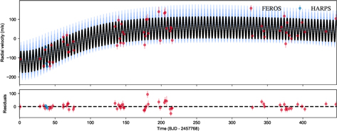
All of our targets showed RV variations at the periods of the observed transits consistent with being of planetary nature, with no indication of being correlated with other stellar parameters (e.g., bisector spans). HATS-56, however, showed an additional long-term trend in its RV signal, which shows no correlation with other parameters (e.g., bisector span). The phase-folded RVs are presented in Figures 3 and 4. We analyze these in detail in Section 3.3.

Figure 3. Phased high-precision RV measurements for HATS-54 (upper left), HATS-55 (upper right), HATS-57 (bottom left), and HATS-58 (bottom right). The RVs for HATS-56 are shown in Figure 4. The instruments used are labeled in the plots. In each case we show three panels. The top panel shows the phased measurements together with our best-fit model (see Table 6) for each system. Zero phase corresponds to the time of midtransit. The center-of-mass velocity has been subtracted. The second panel shows the velocity  residuals from the best fit. The error bars include the jitter terms listed in Table 6 added in quadrature to the formal errors for each instrument. The third panel shows the bisector spans (BS). Note the different vertical scales of the panels.
Download figure:
Standard image High-resolution image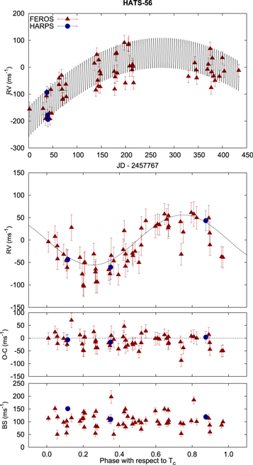
Figure 4. High-precision RV measurements for HATS-56. In the top panel of this figure, we show the RVs plotted vs. time, together with our best-fit model including the orbital wobble of the star due to the planet HATS-56b together with a significant quadratic trend. The bottom three panels are similar to those plotted for the other systems in Figure 3, except here we have subtracted the quadratic trend from the RVs in the panel showing the phase-folded measurements.
Download figure:
Standard image High-resolution image2.3. Photometric Follow-up Observations
Photometric follow-up was obtained for our five systems in order to both refine the transit parameters (including the transit ephemerides) and to rule out possible false-positive scenarios (e.g., blended eclipsing binaries, hierarchical triples). The photometric follow-up included data from the 1 m telescopes at the Las Cumbres Observatory Global Telescope (LCOGT) Network (Brown et al. 2013), the 0.3 m Perth Exoplanet Survey Telescope (PEST), the 1 m Swope Telescope at Las Campanas Observatory (LCO), and the recently commissioned 0.7 m Chilean-Hungarian Automated Telescope (CHAT), also located at LCO. The data reduction for the LCOGT telescopes follows the procedures outlined in Bayliss et al. (2015), which have been updated for automation and will be detailed in a future publication (N. Espinoza et al. 2019, in preparation); this latter set of procedures is similar to the ones used to reduce the Swope telescope data. The data reduction for the PEST telescope is detailed in Zhou et al. (2014). The data reduction for the CHAT telescope follow similar procedures to those described for the LCOGT and Swope data; a full description of CHAT, its reduction, and scheduling will be detailed in a future publication (A. Jordán et al. 2019, in preparation).
Photometric follow-up observations were obtained for HATS-54 with all of the mentioned instruments between 2016 and 2017, with a total of six transits observed in that period (Figure 5). For HATS-55b, transits were observed with PEST, and the Swope and LCO 1 m telescopes (Figure 6). This latter data set is interesting as we observed the same transit of this target from the Cerro Tololo Inter-American Observatory (CTIO) using two different LCOGT 1 m telescopes (on Domes A and C), observing an excellent agreement between both data sets. One transit, a partial transit, and an in-transit portion of the light curve were observed for HATS-56b as well in 2017 from the PEST and LCOGT 1 m telescopes (Figure 7). For HATS-57, photometric follow-up was obtained with the CHAT telescope, including a partial transit of HATS-57b in 2017 August and a full transit in 2017 October (Figure 8). Finally, photometric follow-up was also obtained for HATS-58 in 2017 including two full transits of HATS-58b (Figure 9). The photometric follow-up observations are summarized in Table 1.

Figure 5. Unbinned transit light curves for HATS-54. The light curves have been corrected for quadratic trends in time and for linear trends with up to three parameters characterizing the shape of the PSF, fitted simultaneously with the transit model. The dates of the events, filters, and instruments used are indicated. Light curves following the first are displaced vertically for clarity. Our best fit from the global modeling described in Section 3.3 is shown by the solid lines. The residuals from the best-fit model are shown on the right-hand side in the same order as the original light curves. The error bars represent the photon and background shot noise, plus the readout noise.
Download figure:
Standard image High-resolution image
Figure 6. Same as Figure 5; here we show light curves for HATS-55.
Download figure:
Standard image High-resolution image
Figure 7. Same as Figure 5; here we show light curves for HATS-56.
Download figure:
Standard image High-resolution image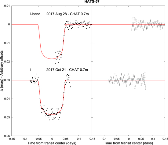
Figure 8. Same as Figure 5; here we show light curves for HATS-57.
Download figure:
Standard image High-resolution image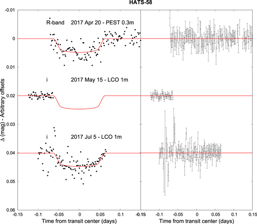
Figure 9. Same as Figure 5; here we show light curves for HATS-58.
Download figure:
Standard image High-resolution image2.4. Lucky Imaging
High spatial resolution imaging via "Lucky imaging" was obtained for HATS-54 and HATS-55 using AstraLux Sur (Hippler et al. 2009) at the New Technology Telescope located in LSO. The data for HATS-54 were obtained on 2015 December 28 with the i' band and for HATS-55 on 2015 December 22 with the z' band. The stacked images, obtained by selecting the best 10% of all the obtained images, are shown in Figure 10, where the plate scale derived in Janson et al. (2017) of 15.2 mas pixel−1 has been used. We analyzed the images using the algorithms described in Espinoza et al. (2016), obtaining an effective FWHM for the stacked HATS-54 observations of 42.36 ± 5.43 mas and for the stacked HATS-55 observations of 52.54 ± 5.50 mas. These are excellent considering the diffraction limit of the instrument is ∼50 mas according to Hippler et al. (2009). The 5σ contrasts curves were generated with the same algorithm, and are presented in Figure 11. No neighboring stars were detected for our targets.
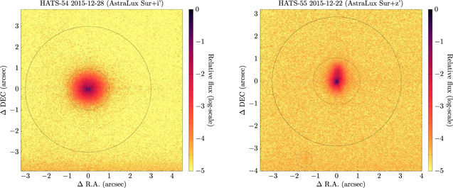
Figure 10. AstraLux lucky images of HATS-54 (left) and HATS-55 (right). No neighboring sources are detected for HATS-54 and HATS-55. The elongated PSF in the HATS-55 image is due to instrumental effects.
Download figure:
Standard image High-resolution image
Figure 11. 5σ contrast curves for HATS-54 (left) and HATS-55 (right) based on our AstraLux Sur z'-band observations. Gray bands show the uncertainty given by the scatter in the contrast in the azimuthal direction at a given radius.
Download figure:
Standard image High-resolution image2.5. Gaia DR2
We queried the coordinates of our target stars into Gaia DR2 (Gaia Collaboration et al. 2018) in order to search for possible companion stars detected by the Gaia mission within 5'' from our targets. No companions were found in Gaia for HATS-54 and HATS-57. We did find companions to our other target stars, which we detail below:
- 1.HATS-55. A very faint source (ΔG = 5.84) was found at ΔR.A. = −1
 52613 ± 0.00032 and Δdecl. = −348374 ± 0.00039 from the target. We note that these coordinates are observable on the field observed by our AstraLux observations and, actually, once these coordinates are known, it is possible to see a faint signal (still within the noise level) in the AstraLux image of HATS-55 (Figure 10). Performing photometry on the AstraLux image at those coordinates, we obtain a magnitude difference of Δz' = 5.30 ± 0.10, which is below our 5σ contrast level (i.e., below the noise level on our image). From Gaia, the proper motion of the target and the companion are inconsistent with each other, which implies they are not physically bound.
 - 2.HATS-56. A faint (ΔG = 3.94) source was found at ΔR.A. = −148296 ± 0.00026 and Δdecl. = 059747 ± 0.00044 from this target, the proper motion (−9.19 ± 0.57 mas yr−1 in R.A., −3.00 ± 0.74 mas yr−1 in decl.) of which is consistent with that of the target (−8.604 ± 0.046 mas yr−1 in R.A., −2.950 ± 0.035 mas yr−1 in decl.), which could imply it is physically bound. However, it is unclear whether the Gaia parallax is reliable enough to claim this latter hypothesis as true, as it is very uncertain for the faint companion to HATS-56. In any case, the neighbor is faint enough relative to the target star that it can be ignored in the analysis.
- 3.HATS-58. A bright source (ΔG = 0.92 fainter than the target star) was found at ΔR.A. = 029733 ± 0.00051 and Δdecl. = −068025 ± 0.00028 from our target. The proper motion of this object measured by Gaia DR2 (−12.96 ± 0.92 mas yr−1 in R.A., −2.30 ± 0.44 mas yr−1 in decl.) is consistent with the proper motion of our target (−12.70 ± 0.30 mas yr−1 in R.A., −3.23 ± 0.16 mas yr−1 in decl.) and, therefore, we assume they are physically bound. Because of this, from now on in this work we refer to the brighter star as HATS-58A and to the fainter companion as HATS-58B. The Gaia photometry gives a very uncertain effective temperature for HATS-58B of
 K. This neighbor is sufficiently bright relative to the target star that it must be taken into account.

3. Analysis
3.1. Properties of the Parent Star
In order to determine the parameters of the parent stars of our planetary candidates, we obtained precise stellar atmospheric parameters using the Zonal Atmospherical Stellar Parameter Estimator (ZASPE; Brahm et al. 2017b), by using the stacked HARPS spectra for HATS-55 and the stacked FEROS spectra for the rest of our targets. With these atmospheric parameters, we performed a joint analysis with all available data following the method explained in detail in Hartman et al. (2019; see Section 3.3 for a brief overview) in order to obtain the physical parameters of the stars. With these physical parameters in hand, a second ZASPE iteration was performed for all targets, where the revised value of the log gravity was used as input in order to derive the final atmospheric parameters of the stars; these were then used again in a second iteration of the joint modeling to be detailed in Section 3.3 to obtain the final parameters of the stars, which are presented in Table 5. We present the locations of our target stars on the absolute G magnitude versus Gaia DR2 BP – RP colors in Figures 14 and 15 for all our targets except for HATS-58A, for which we present it in the absolute G magnitude versus effective temperature plane as this target did not have a well-measured BP – RP color. In addition, as will be detailed in Section 3.3, the analysis for this latter star was special as it is blended with HATS-58B in all of our measurements with the exception of Gaia, where the two components of the blend are resolved, as mentioned in the previous section. We account for this in our modeling, and we were able to obtain a mass for HATS-58B of  M⊙.
M⊙.
Table 5. Stellar Parameters for HATS-54–HATS-58A
| HATS-54 | HATS-55 | HATS-56 | HATS-57 | HATS-58 | ||
|---|---|---|---|---|---|---|
| Parameter | Value | Value | Value | Value | Value | Source |
| Astrometric properties and cross-identifications | ||||||
| Gaia DR2-ID | 6087996849371141248 | 5592019557950033536 | 6144125887172751232 | 5094406193214399616 | 6128363666439822208 | |
| 2MASS-ID | 13223237-4441196 | 07370802-3245195 | 12003962-4547579 | 04034760-1903242 | 12270898-4858423 | |
| GSC-ID | GSC 7799-01184 | GSC 7109-00596 | GSC 8229-02228 | GSC 5885-00663 | GSC 8239-00065 | |
| R.A. (J2000) |

|

|

|

|

|
Gaia DR2 |
| Decl. (J2000) |

|

|

|

|

|
Gaia DR2 |
μR.A. ( ) ) |

|

|

|

|

|
Gaia DR2 |
μDecl. ( ) ) |

|

|

|

|

|
Gaia DR2 |
| Parallax (mas) |

|

|

|

|

|
Gaia DR2 |
| Spectroscopic properties | ||||||
 (K) (K) |

|

|

|

|

|
ZASPEa |
![$[\mathrm{Fe}/{\rm{H}}]$](https://content.cld.iop.org/journals/1538-3881/158/2/63/revision1/ajab26bbieqn54.gif)
|

|

|

|

|

|
ZASPE |
 ( ( ) ) |

|

|

|

|

|
ZASPE |
 ( ( ) ) |

|

|

|

|

|
Assumed |
 ( ( ) ) |

|

|

|

|

|
Assumed |
γRV ( )... )... |

|

|

|

|

|
FEROS/HARPSb |
 ( ( d−1) d−1) |
⋯ | ⋯ |

|
⋯ | ⋯ | FEROS/HARPSc |
 ( ( d−2)... d−2)... |
⋯ | ⋯ |

|
⋯ | ⋯ | FEROS/HARPSc |
| Photometric properties | ||||||
| B (mag) |

|

|

|

|

|
APASSd |
| V (mag) |

|

|

|

|

|
APASSd |
| g (mag) |

|

|

|

|

|
APASSd |
| r (mag) |

|

|

|

|

|
APASSd |
| i (mag) |

|

|

|

|

|
APASSd |
| G (mag) |
|
|

|

|

|
Gaia DR2 |
| BP (mag) |

|

|

|

|
⋯ | Gaia DR2 |
| RP (mag) |

|

|

|

|
⋯ | Gaia DR2 |
| J (mag) |

|

|

|

|

|
2MASS |
| H (mag) |

|

|

|

|

|
2MASS |
| Ks (mag) |

|

|

|

|

|
2MASS |
| Derived properties | ||||||
 ( ( ) ) |

|

|

|

|

|
Joint fite |
 ( ( ) ) |

|

|

|

|

|
Joint fit |
| Teff (K) |

|

|

|

|

|
Joint fit |
 (cgs) (cgs) |

|

|

|

|

|
Joint fit |
| Fe/H (dex) |

|

|

|

|
⋯ | Joint fit |
 ( ( ) ) |

|

|

|

|

|
Joint fit |
 ( ( ) ) |

|

|

|

|

|
Joint fit |
| Age (Gyr) |

|

|

|

|

|
Joint fit |
| AV (mag) |

|

|

|

|

|
Joint fit |
| Distance (pc) |

|

|

|

|

|
Joint fit |
Notes. The adopted parameters for all five systems are from a model in which the orbit is assumed to be circular. For HATS-58, all the values refer to the brightest of the components of the two-component stellar system (HATS-58A)—note that all photometry but that of Gaia is blended for this star. See the discussion in Section 3.3.
aZASPE = Zonal Atmospherical Stellar Parameter Estimator routine for the analysis of high-resolution spectra (Brahm et al. 2017b), applied to the FEROS spectra of each system. These parameters rely primarily on ZASPE, but have a small dependence also on the iterative analysis incorporating the isochrone search and global modeling of the data. bThe listed γRV is from FEROS for HATS-54, HATS-56, HATS-57, and HATS-58. For HATS-55, it is from HARPS. The error on γRV is determined from the orbital fit to the RV measurements and does not include the systematic uncertainty in transforming the velocities to the IAU standard system. The velocities have not been corrected for gravitational redshifts. cFor HATS-56, the RVs show a significant quadratic trend in addition to the Keplerian orbital variation, due to the transiting planet HATS-56b (Figure 4). This trend is modeled as , where
  is the center time of the first transit observed in the HATSouth light curve.
dFrom APASS DR6 as listed in the UCAC 4 catalog (Zacharias et al. 2012).
eObtained through the joint fit detailed in Hartman et al. (2019) and briefly summarized in Section 3.3.
is the center time of the first transit observed in the HATSouth light curve.
dFrom APASS DR6 as listed in the UCAC 4 catalog (Zacharias et al. 2012).
eObtained through the joint fit detailed in Hartman et al. (2019) and briefly summarized in Section 3.3.
As mentioned in Section 2.1, we observe that HATS-57 shows variability at the 2% level. This variability could be used to estimate the rotation period of the star which, combined with the value of  given in Table 5, could in turn give us an estimate of the inclination of the star with respect to the line of sight, i*. To find the period of this modulation, we model the light curve using a Gaussian Process (GP) regression. We use the quasi-periodic kernel presented in Foreman-Mackey et al. (2017) of the form
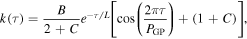
where τ = ti − tk, with ![$i,k\in [1,2,\,\ldots \,N]$](https://content.cld.iop.org/journals/1538-3881/158/2/63/revision1/ajab26bbieqn207.gif) , where N is the number of data points, and B, C, L and PGP are the hyperparameters of the model, with the last one corresponding to the period of the quasi-periodic oscillations defined by this kernel. We assume that the light curve has a zero-point flux and an extra jitter, which we also model. In order to efficiently explore the full parameter space, we use MultiNest (Feroz et al. 2009) with the PyMultinest Python wrapper (Buchner et al. 2014) to find the posterior density of the parameters of the GP. This code, which we call GPRotatioNest, is available at GitHub.21
, where N is the number of data points, and B, C, L and PGP are the hyperparameters of the model, with the last one corresponding to the period of the quasi-periodic oscillations defined by this kernel. We assume that the light curve has a zero-point flux and an extra jitter, which we also model. In order to efficiently explore the full parameter space, we use MultiNest (Feroz et al. 2009) with the PyMultinest Python wrapper (Buchner et al. 2014) to find the posterior density of the parameters of the GP. This code, which we call GPRotatioNest, is available at GitHub.21
Using GPRotatioNest on the light curve of HATS-57, we find two modes for the period, one at 6.355 ± 0.018 days, which is the dominant peak in the posterior distribution, and another one at 11.27 ± 0.57 days. When phasing the data with both periods, it is evident that the former does a significantly better job at coherently adding the periodicity; however, from the same phasing of the data it is obvious that this is half the real periodicity as well. Based on this, we interpret 2PGP, i.e., 12.71 ± 0.037 days, as the rotation period of the star. Figure 12 shows a portion of the data for the light curve of HATS-57, along with the prediction from the GP, whereas Figure 13 shows the photometry phased at this period. With this period, the  , and the radius of the star presented in Table 5, we derive an inclination of the star with respect to the line of sight of
  degrees.
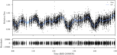
Figure 12. (Top) Portion of the light curve of HATS-57 (black points) along with the posterior GP model (blue line—darker blue bands denote the 3σ credibility bands around it). (Bottom) Residuals between the GP and the data in parts per million (ppm).
Download figure:
Standard image High-resolution image
Figure 13. Phased light curve of HATS-57 to the period of 12.71 days found via our GP regression (see text and Figure 12). Black points show the original data, whereas blue circles show the binned light curve.
Download figure:
Standard image High-resolution image3.2. Excluding Blend Scenarios
In order to exclude blend scenarios, we carried out an analysis following Hartman et al. (2012) and the updates to the procedure outlined in Hartman et al. (2019), which allows us to account for the information in Gaia DR2 together with all the available photometric and spectroscopic data presented in previous sections. We attempt to model the available photometric data (including light curves and catalog broadband photometric measurements) for each object as (1) a hierarchical triple-star system where the two fainter stars form an eclipsing binary, (2) a blend between a bright foreground star and a fainter background eclipsing binary star system, and (3) a bright star with a transiting planet and a fainter unresolved stellar companion. The possibilities are then rejected based on that data or based on the RVs and bisector span variations they would imply. We constrain the physical properties of the stars in these systems using the PARSEC stellar evolutionary models (Marigo et al. 2017) along with the MWDUST 3D Galactic extinction model (Bovy et al. 2016), which is used in order to place priors on the extinction coefficient AV. The results for each system are as follows:
- 1.HATS-54—the best-fit blend model, which corresponds to the blend between a bright foreground star and a fainter background eclipsing binary system, has a slightly higher χ2 than the best-fit model of a single star with a planet based solely on the photometry (Δχ2 = 4.7). However, simulated bisector span and RV observations for blend models that come close to matching the photometry cannot reproduce the observed bisector span and RV measurements.
- 2.HATS-55—all blend models can be rejected in favor of a model of a single star with a planet based solely on the photometry.
- 3.HATS-56—the best-fit blend model, which corresponds to the blend between a bright foreground star and a fainter background eclipsing binary system, has a slightly higher χ2 than the best-fit model of a single star with a planet based solely on the photometry (Δχ2 = 13.6). However, as with HATS-54, simulated bisector span and RV observations for blend models that come close to matching the photometry cannot reproduce the observed bisector span and RV measurements. In particular, the simulated bisector spans show scatters in excess of 100 m s−1, which we do not observe in our data.
- 4.HATS-57—all blend models can be rejected in favor of a model of a single star with a planet based solely on the photometry.
- 5.HATS-58A—The blend analysis in this case was special as all of our data but the Gaia DR2 photometry is blended with the companion star HATS-58B. The blend analysis is performed assuming the two sources are a binary and trying each as a potential object that either hosts a planet, or is blended with an eclipsing binary. The blend models in which HATS-58A is the blending source are ruled out using the photometry alone. The blending model in which HATS-58B is a hierarchical triple-star system, however, cannot be ruled out using only the photometry. However, this can be rejected based on simulated RVs implied by such a system. To perform these simulations, we selected a random subset of the links from a Markov Chain Monte Carlo (MCMC) modeling of this scenario and calculated simulated RVs and simulated bisector span variations for each scenario. We found that the simulated RVs have amplitudes larger than about 2 km s−1, and the simulated bisector span variations have a scatter larger than 400 m s−1, both of which are inconsistent with our observations. The blending model in which HATS-58B is a blend between a bright foreground star and a fainter background eclipsing binary system has actually a lower chi-square than the model in which HATS-58A hosts a transiting exoplanet (Δχ2 = −38.6). However, this scenario can also be rejected when the implied RVs and bisector spans for this scenario are compared to our data: they imply RV amplitudes in excess of 1 km s−1 and bisector span variations with scatters larger than about 700 m s−1, both of which are inconsistent with our observations. Based solely on the photometry, we cannot differentiate between the scenarios in which either HATS-58A or HATS-58B hosts the transiting exoplanet. However, the clean orbital variation measured with HARPS suggests HATS-58A is the star hosting the exoplanet, and this is the model we select for this system.
As is generally the case, we cannot rule out in all of the above detailed cases whether there are additional unresolved faint foreground and/or physically associated stars contaminating our measurements. We can, however, put limits on the masses of possible companion stars: based on our analysis, we place 95% confidence upper limits on the masses of any unresolved stellar companions of 0.28  for HATS-54, 0.15
  for HATS-55, and 0.41
  for HATS-57. For HATS-56, if the faint detected Gaia source is indeed physically bound to it, it would have a mass of 0.8058 ± 0.0076
  .
.
3.3. Global Modeling of the Data
The global modeling of the photometric and RV data was made following the method recently introduced in detail in Hartman et al. (2019), which simultaneously models the light curves, RVs, atmospheric parameters (effective temperature and metallicity), the Gaia DR2 parallax, and Gaia broadband photometry. Light curves are modeled using the formalism outlined in Mandel & Agol (2002). RV modeling assumes Keplerian orbits, and stellar parameters and parallax are modeled using the PARSEC stellar evolution models (Marigo et al. 2017). A Differential Evolution MCMC procedure was used to explore the parameter space and obtain the posterior distributions for our systems. This same procedure was applied to all of our targets except for the HATS-58 system, for which a blended object (in all of our observations and in non-Gaia broadband photometric measurements) is detected in Gaia DR2 at 074239 ± 000032 from the target. This latter pair of blended stars, in turn, have common proper motions and consistent parallaxes, which indicate that they form a bound system. We model both stars simultaneously in our fits and do not consider their Gaia BP and RP measurements as they are unreliable.
Fits using both circular and eccentric models were tried for all of our systems, and the method of Weinberg et al. (2013) was used to estimate the Bayesian evidence for each scenario. In all cases, the eccentricity is consistent with zero. The resulting parameters for each system are listed in Table 6; the photometric fits are shown in Figure 1 for the HATSouth discovery photometry: Figures 5 through 9 for the follow-up light curves, Figures 3 and 4 for the RVs, Figures 14 and 15 show the stellar evolutionary tracks in the Gaia BP – RP versus absolute G magnitude Hertzsprung–Russell diagram for all stars except HATS-58(A), where the same tracks are shown in the effective temperature–absolute G-magnitude plane and, finally, Figures 16 and 17 show the broadband spectral energy distribution (SED) fits to the observed bands, with the latter figure showing the one corresponding to both stellar components of the HATS-58 system, HATS-58A and HATS-58B.
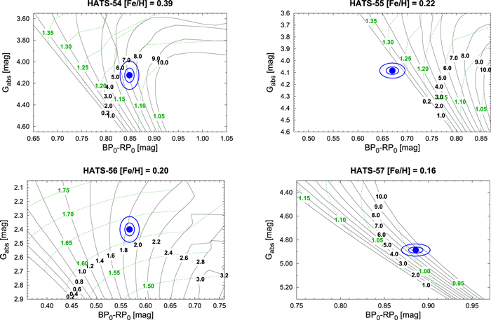
Figure 14. Model isochrones (black solid lines) from Yi et al. (2001) for the measured metallicities of HATS-54 (upper left), HATS-55 (upper right), HATS-56 (bottom left), and HATS-57 (bottom right). HATS-58A is shown in Figure 15. The age of each isochrone in gigayears is labeled in black. We also show evolutionary tracks for stars of fixed mass (dashed green lines) with the mass of each tracked labeled in solar mass units in green. The dereddened BP0 − RP0 colors and absolute G magnitudes from Gaia DR2 are shown for each host star using filled blue circles together with their 1σ and 2σ confidence ellipsoids (blue lines).
Download figure:
Standard image High-resolution image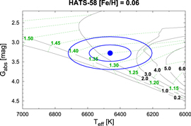
Figure 15. Same as Figure 14; here we show HATS-58A. In this case, however, we use the spectroscopically determined stellar effective temperature value instead of BP0 − RP0, as this target did not have a well-measured BP – RP color (see text).
Download figure:
Standard image High-resolution image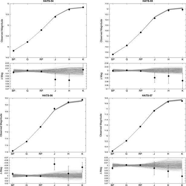
Figure 16. Best-fit SED posterior samples from our joint modeling (gray lines) for Gaia's BP, G, and RP bands and 2MASS J, H, and K bands (black points) for HATS-54 (upper left), HATS-55 (upper right), HATS-56 (bottom left), and HATS-57 (bottom right). The one for the HATS-58 system is shown in Figure 17.
Download figure:
Standard image High-resolution image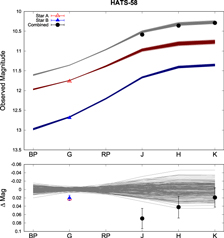
Figure 17. Same as Figure 14; here for the HATS-58 system. In this case, however, we show the fits for both stellar components (HATS-58A, red, and HATS-58B, blue lines), which are blended in the J, H, and K 2MASS photometry (black dots), but resolved in Gaia's G band (red and blue triangles).
Download figure:
Standard image High-resolution imageTable 6. Orbital and Planetary Parameters for HATS-54b–HATS-58Ab
| HATS-54b | HATS-55b | HATS-56b | HATS-57b | HATS-58Ab | |
|---|---|---|---|---|---|
| Parameter | Value | Value | Value | Value | Value |
| Light curve parameters | |||||
| P (days) |

|

|
|

|

|
| Tc (BJD)a |

|

|

|

|

|
| T14 (days)a |

|

|

|
|

|
| T12 = T34 (days)a |

|

|
|

|

|

|

|

|

|

|

|
 b b
|

|

|

|

|

|
 / /
|

|

|

|

|

|
| b2 |

|

|

|

|

|

|

|

|

|

|

|
| i (deg) |

|

|

|

|

|
| HATSouth dilution factorsd | |||||
| Dilution factor 1 |

|

|

|

|
⋯ |
| Dilution factor 2 | ⋯ | ⋯ |

|
⋯ | ⋯ |
| Limb-darkening coefficientse | |||||
| c1, g |

|
⋯ | ⋯ | ⋯ | ⋯ |

|

|
⋯ | ⋯ | ⋯ | ⋯ |
| c1, r |

|

|

|

|

|
| c2, r |

|

|

|

|

|
| c1, R |

|

|

|
⋯ |

|
| c2, R |

|

|

|
⋯ |

|
| c1, i |

|

|

|

|

|
| c2, i |

|

|

|

|

|
| RV parameters | |||||
K ( ) ) |

|

|

|

|

|
| ef | <0.126 | <0.092 | <0.019 | <0.028 | <0.168 |
RV jitter FEROS ( )g )g
|

|
⋯ |

|

|

|
RV jitter HARPS ( ) ) |
<242.8 | <9.3 | <10.3 | ⋯ | <19.2 |
| Planetary parameters | |||||
 ( ( ) ) |

|

|

|

|

|
 ( ( ) ) |

|

|

|

|

|
 h h
|

|

|

|

|
⋯ |
 ( ( ) ) |

|

|

|

|

|
 (cgs) (cgs) |

|

|

|

|

|
| a (AU) |

|

|

|

|

|
| Teq (K) |

|

|

|

|

|
| Θ i |

|

|

|

|

|
 (cgs)j (cgs)j
|

|

|

|

|

|
Notes. For all five systems, we adopt a model in which the orbit is assumed to be circular. See the discussion in Section 3.3.
aTimes are in Barycentric Julian Date calculated directly from UTC without correction for leap seconds. Tc: reference epoch of the midtransit that minimizes the correlation with the orbital period. T12: total transit duration, time between first to last contact; T12 = T34: ingress/egress time, time between first and second, or third and fourth, contact. bReciprocal of the half-duration of the transit used as a jump parameter in our MCMC analysis in place of . It is related to
  by the expression
  (Bakos et al. 2010).
dScaling factor applied to the model transit that is fit to the HATSouth light curves. This factor accounts for dilution of the transit due to blending from neighboring stars and overfiltering of the light curve. These factors are varied in the fit, with independent values adopted for each HATSouth light curve. The factors listed HATS-54, HATS-55, HATS-57, and HATS-58 are for the G700.3, G602.4, G548.3, and G699.1 light curves, respectively. For HATS-56, we list the factors for the G698.1 and G698.4 light curves in order.
eValues for a quadratic law, adopted from the tabulations by Claret (2004) according to the spectroscopic (ZASPE) parameters listed in Table 5.
fThe 95% confidence upper limit on the eccentricity determined when
(Bakos et al. 2010).
dScaling factor applied to the model transit that is fit to the HATSouth light curves. This factor accounts for dilution of the transit due to blending from neighboring stars and overfiltering of the light curve. These factors are varied in the fit, with independent values adopted for each HATSouth light curve. The factors listed HATS-54, HATS-55, HATS-57, and HATS-58 are for the G700.3, G602.4, G548.3, and G699.1 light curves, respectively. For HATS-56, we list the factors for the G698.1 and G698.4 light curves in order.
eValues for a quadratic law, adopted from the tabulations by Claret (2004) according to the spectroscopic (ZASPE) parameters listed in Table 5.
fThe 95% confidence upper limit on the eccentricity determined when  and
and  are allowed to vary in the fit.
gTerm added in quadrature to the formal RV uncertainties for each instrument. This is treated as a free parameter in the fitting routine. In cases where the jitter is consistent with zero, we list its 95% confidence upper limit.
hCorrelation coefficient between the planetary mass
are allowed to vary in the fit.
gTerm added in quadrature to the formal RV uncertainties for each instrument. This is treated as a free parameter in the fitting routine. In cases where the jitter is consistent with zero, we list its 95% confidence upper limit.
hCorrelation coefficient between the planetary mass  and radius
  estimated from the posterior parameter distribution.
iThe Safronov number is given by
estimated from the posterior parameter distribution.
iThe Safronov number is given by  (see Hansen & Barman 2007).
jIncoming flux per unit surface area, averaged over the orbit.
(see Hansen & Barman 2007).
jIncoming flux per unit surface area, averaged over the orbit.
For the HATS-58 system, we adopt the parameters determined through the blend analysis described in Section 3.2. This analysis makes use of the JKTEBOP detached eclipsing binary light curve model (Nelson & Davis 1972; Etzel 1981; Popper & Etzel 1981; Southworth et al. 2004a, 2004b) in place of the Mandel & Agol (2002) transit models. We also treat the stellar masses (for both the planet host and its binary star companion) and the system age as jump parameters in this analysis, rather than the inverse half-duration of the transit and the stellar effective temperature.
As can be seen, HATS-54b, HATS-55b, and HATS-58Ab are very similar in terms of densities, consistent with being typical hot Jupiters. On the other hand, HATS-56b is highly inflated and has a very low density of only  g cm−3, while HATS-57b is massive. We discuss the retrieved parameters of the systems in the next section.
4. Discussion
Figure 18 puts our newly discovered exoplanets in the context of known and well-studied exoplanets (with radii and masses estimated to better than 20%) in both the equilibrium temperature/radius and the mass/radius diagrams. As can be observed, the parameters of HATS-54b, HATS-55b, and HATS-58Ab make them consistent with being part of the well-represented population of inflated hot Jupiters, with HATS-54b and HATS-58Ab falling in terms of equilibrium temperature on the interesting regime of maximum heating efficiency for inflation proposed by Thorngren & Fortney (2018). In addition, as discussed in Section 2.5, both HATS-56 and HATS-58 are most likely systems composed of at least two stars. On one hand, given the separation observed by Gaia DR2 between HATS-55 and the companion of 380336 ± 0.00038, and the calculated distance to the system of 623.6 ± 6.2 pc, the projected separation of the stars assuming they are bound is 2361 ± 23 au. On the other hand, given the separation observed by Gaia DR2 between HATS-58A and HATS-58B of 074238 ± 0.00033 and the calculated distance to the system of 492 ± 21 pc, the projected separation of the stars assuming they are bound is 365 ± 15 au.

Figure 18. Equilibrium-temperature–radius and mass–radius diagrams of known exoplanets obtained from TEPcat (Southworth 2011). Colored points with error bars indicate HATS-54b to HATS-58Ab, with colors indicating the planetary effective temperature of our newly discovered transiting exoplanets. The color is consistent between both diagrams.
Download figure:
Standard image High-resolution imageHATS-57b, on the other hand, is a dense ( gr cm−3) and quite massive hot Jupiter that seems to fall within the expected size given its equilibrium temperature, especially if one considers that inflation is slightly less pronounced for more massive planets (Sestovic et al. 2018). The planet's radius and mass are consistent with the models of Thorngren & Fortney (2018) for HATS-57b's equilibrium temperature of
  K, suggesting that the inflation mechanism is indeed operating in HATS-57b just like in every other hot Jupiter with a similar equilibrium temperature. Interestingly, the expected amplitude of the Rossiter–Mclaughlin (RM) effect on this system is of order
  m s−1; this is about one-half of the total observed uncertainties on the RVs observed in our high-precision RV follow-up, and thus this could be a good system to characterize with this effect. The system is particularly interesting because according to the derived stellar period in Section 3.1, the star shows hints of being slightly misaligned with respect to the plane of the sky (
 degrees). Given the nearly edge-on inclination of the planetary system with respect to the plane of the sky (i = 87
 88 ± 040), this hints that this may be a misaligned system, a hypothesis that can be tested with RM measurements.
Finally, HATS-56b is highly inflated and possesses a very low density of  gr cm−3. Its inflated nature is, however, not rare given its relatively large equilibrium temperature of
  K, which in turn makes it a very good candidate for future atmospheric follow-up, especially given the brightness of the host star (V = 11.6). The expected atmospheric scale height for HATS-56b is around 1100 km, which in turn implies an expected signal in transmission between 120 and 360 ppm, around 70% the expected transmission signal for HD 209458b. An additional very interesting feature of this hot Jupiter is that it shows a significant quadratic trend in its RVs (see Figure 4) that could imply an additional companion. In order to see what this latter interpretation would mean if it actually were another planet around HATS-56, we used juliet22
(Espinoza et al. 2018), a tool that allows us not only to fit multiplanetary systems but also to estimate the Bayesian evidence, Z, of different models, in order to fit a two-planet solution to the RVs. To do this, juliet couples radvel (Fulton et al. 2018) with MultiNest in order to perform the posterior sampling and to calculate said Bayesian evidences. We used the already-derived properties of HATS-56b (defined mainly by its transits) as inputs. We fix in our two-planet fit the eccentricity of HATS-56b to zero and give as priors for this planet the posteriors on the period and time-of-transit center presented in Table 6; with this, we perform a two-planet fit to the RV data in order to explore the parameter space using wide priors on the parameters for the candidate planet HATS-56c (a Jeffreys prior for the period from 5 to 10,000 days, a time of transit center uniform between 2,457,700 and 2,467,700, a uniform prior for the semiamplitude between 0 and 1000 m s−1), and wide priors for the semiamplitude of the known transiting planet (uniform between 0 and 100 m s−1), allowing eccentric orbits for the outer planet.
K, which in turn makes it a very good candidate for future atmospheric follow-up, especially given the brightness of the host star (V = 11.6). The expected atmospheric scale height for HATS-56b is around 1100 km, which in turn implies an expected signal in transmission between 120 and 360 ppm, around 70% the expected transmission signal for HD 209458b. An additional very interesting feature of this hot Jupiter is that it shows a significant quadratic trend in its RVs (see Figure 4) that could imply an additional companion. In order to see what this latter interpretation would mean if it actually were another planet around HATS-56, we used juliet22
(Espinoza et al. 2018), a tool that allows us not only to fit multiplanetary systems but also to estimate the Bayesian evidence, Z, of different models, in order to fit a two-planet solution to the RVs. To do this, juliet couples radvel (Fulton et al. 2018) with MultiNest in order to perform the posterior sampling and to calculate said Bayesian evidences. We used the already-derived properties of HATS-56b (defined mainly by its transits) as inputs. We fix in our two-planet fit the eccentricity of HATS-56b to zero and give as priors for this planet the posteriors on the period and time-of-transit center presented in Table 6; with this, we perform a two-planet fit to the RV data in order to explore the parameter space using wide priors on the parameters for the candidate planet HATS-56c (a Jeffreys prior for the period from 5 to 10,000 days, a time of transit center uniform between 2,457,700 and 2,467,700, a uniform prior for the semiamplitude between 0 and 1000 m s−1), and wide priors for the semiamplitude of the known transiting planet (uniform between 0 and 100 m s−1), allowing eccentric orbits for the outer planet.
Figure 19 shows our modeling of the RV assuming a two-planet model for them. As expected, we recover the same semiamplitude for HATS-56b derived in previous sections, while for the possible planet HATS-56c, we obtain a highly uncertain period of Pc =  days and a time of transit center of
  days (BJD UTC), coupled with a possible eccentric orbit with ec = 0.46 ± 0.07 and
  degrees, and a semiamplitude of
  m s−1. It is interesting to note that this model is favored over a fit with a simple quadratic trend (
 in favor of the two Keplerians). These values imply a minimum mass for the possible planet c of
  . Perhaps the most interesting feature of the possible planet HATS-56c is its derived distance from the star and, hence, its equilibrium temperature. We use the very tight constraint on the stellar density for the star and the derived period for this possible planet to derive a value
  from Kepler's third law (1.99 ± 0.43 au). Combining this with the stellar effective temperature, we obtain a zero-albedo equilibrium temperature for the possible planet HATS-56c of Teq = 332 ± 50 K, which would imply a temperate companion that would fall very close to the habitable zone of the star. If confirmed, HATS-56c would be a very interesting system to study, due to the possibility that satellites orbiting it could present habitable conditions in terms of the stellar irradiation.
Figure 19. Two-planet modeling of the radial velocities (red points, FEROS; blue points, HARPS) for HATS-56. The best-fit radial-velocity model is shown in solid black line with blue bands denoting the 68%, 95% and 99% credibility interval. The bottom panel shows the residuals of the fit in m s−1.
Download figure:
Standard image High-resolution image
It is interesting to note that on top of the exciting feature of the HATS-56 system being a multicomponent system, Gaia DR2 data reveal an additional (possibly bound, stellar) companion to HATS-56. Given the observed separation of this companion from HATS-56 of 159879 ± 0.00029 and the derived distance to the system of 577.1 ± 9.6 pc, if physically bound, the companion would be at least at a distance of 922 ± 15 au (which is inconsistent with the derived distance of HATS-56c). This is inconsistent with the derived range of distances that could give rise to the observed RV long-term trend, and as such, this cannot explain it given our data.
Confirmation of the candidate exoplanet HATS-56c could be performed if further RV follow-up is performed within the next ∼2 yr. The expected time of periastron passage, taking our best-fit model for the candidate, is expected to occur around mid-2020, but monitoring the decrease of the RV curve as it approaches this point will be very important to both predict the exact time of periastron passage (in order to increase the sampling of the RV follow-up) and to constrain the exact shape of the RV curve, which has useful information for constraining the orbit of the possible planet. Regarding possible transits, given the current uncertainty on the period and time of transit center, catching a possible transit event of the candidate planet is rather difficult. We inspected the HATSouth photometry but we found it is not precise enough to provide any constraints on possible events; the errors on the transit parameters are so large that it is very difficult to analyze the light curve, especially considering that we are most likely searching for only one transit. With further RV follow-up, however, this search could be made even in the current HATSouth light curves, which could be joined with other photometric surveys in order to search for the possible transit signature of HATS-56c. In fact, the TESS mission (Ricker et al. 2015) will observe HATS-56 during its passage through Sector 2, and this could provide a brief but interesting search for this extra possible signal
5. Conclusions
In this work, we have presented the discovery of HATS-54b through HATS-58Ab. HATS-54b, HATS-55b, and HATS-58Ab are typical hot Jupiters in many aspects, but sample the interesting effective temperature range where the maximum heating efficiency for inflation is proposed to occur (Thorngren & Fortney 2018). HATS-56b and HATS-57b, however, are special: the latter is a dense hot Jupiter that could be a good target for RM observations and orbits an apparently active star showing peak-to-peak variability on the order of 2%, whereas HATS-56b is not only an excellent target for future atmospheric follow-up but also for future RV monitoring in order to confirm the planetary nature of an evident long-term RV signal observed during our high-resolution spectroscopic follow-up. If we assume this latter signal is actually from an additional planet in the system, this would be a super-Jupiter with a minimum mass of  and could orbit close to the habitable zone of HATS-56, which would be interesting in terms of habitability if there are satellites orbiting the possible planet HATS-56c. RV monitoring of this system during the next two years will be very useful in order to both constrain the time of periastron passage (expected to occur in 2020) and to constrain the possible times of transit center of this external possible companion.
Development of the HATSouth project was funded by NSF MRI grant NSF/AST-0723074, operations have been supported by NASA grants NNX09AB29G, NNX12AH91H, and NNX17AB61G, and follow-up observations have received partial support from grant NSF/AST-1108686. N.E. acknowledges support from the Gruber Foundation. A.J. acknowledges support from FONDECYT project 1171208, CONICYT project BASAL AFB-170002, and by the Ministry for the Economy, Development, and Tourism's Programa Iniciativa Científica Milenio through grant IC 120009, awarded to the Millennium Institute of Astrophysics (MAS). M.R. acknowledges support from CONICYT project Basal AFB-170002. R.B. acknowledges support from project IC120009 "Millenium Institute of Astrophysics (MAS)" of the Millennium Science Initiative, Chilean Ministry of Economy. V.S. acknowledges support form BASAL CATA PFB-06. A.V. is supported by the NSF Graduate Research Fellowship, grant No. DGE 1144152. This work is based on observations made with ESO Telescopes at the La Silla Observatory. This paper also uses observations obtained with facilities of the Las Cumbres Observatory Global Telescope. We acknowledge the use of the AAVSO Photometric All-Sky Survey (APASS), funded by the Robert Martin Ayers Sciences Fund, and the SIMBAD database, operated at CDS, Strasbourg, France. Operations at the MPG 2.2 m Telescope are jointly performed by the Max Planck Gesellschaft and the European Southern Observatory. The imaging system GROND has been built by the high-energy group of MPE in collaboration with the LSW Tautenburg and ESO. We thank the MPG 2.2 m telescope support team for their technical assistance during observations." This work has made use of data from the European Space Agency (ESA) mission Gaia (https://www.cosmos.esa.int/gaia), processed by the Gaia Data Processing and Analysis Consortium (DPAC, https://www.cosmos.esa.int/web/gaia/dpac/consortium). Funding for the DPAC has been provided by national institutions, in particular the institutions participating in the Gaia Multilateral Agreement.
Footnotes
- *
The HATSouth network is operated by a collaboration consisting of Princeton University (PU), the Max Planck Institute für Astronomie (MPIA), the Australian National University (ANU), and the Pontificia Universidad Católica de Chile (PUC). The station at Las Campanas Observatory (LCO) of the Carnegie Institute is operated by PU in conjunction with PUC, the station at the High Energy Spectroscopic Survey (H.E.S.S.) site is operated in conjunction with MPIA, and the station at Siding Spring Observatory (SSO) is operated jointly with ANU. Based in part on observations made with the MPG 2.2 m Telescope at the ESO Observatory in La Silla.
- 20
- 21
- 22