


Abstract
The Wilson–Devinney program has been used to analyze well-calibrated photometric and new radial velocity data to determine the properties and distance of DS Andromedae, a 1.01 day period, double-lined, totally eclipsing binary system of early-F spectral type and a likely member of the intermediate-age open cluster NGC 752. The determinations of many of the system elements including the distance are robust against modest changes in model assumptions. Third light is present in all passbands at the 10% level. The weighted means of the best-fitting model yield a distance of 477 ± 4 ±12 pc, equivalent to (m – M)0 = 8.390 ± 0.018 ± 0.060 mag, and masses of 1.655 ± 0.003 ± 0.030 MSun and 1.087 ±0.005 ± 0.040 MSun, radii of 2.086 ± 0.003 ± 0.013 and 1.255 ± 0.005 ± 0.012 RSun, and effective temperatures 7056 ± 21 ± 140 RSun and 5971 ± 33 ± 130 K, for components 1 and 2, respectively, where the formal internal uncertainties are followed by conservatively estimated systematic errors. Possible but less satisfactory semidetached models produce more parameter variations and larger mean residuals. The primary star is seen to be at or very close to the main-sequence turnoff at an age of 1.55 ± 0.05 Gyr but appears to be too small for its mass, whereas the secondary appears to be too luminous for its temperature and too large for its mass compared to models of single stars.
Export citation and abstract BibTeX RIS
1. Introduction
The potential synergy presented by an eclipsing, double-lined spectroscopic binary (hereafter ESB2) within a star cluster has been a motivation for one of us (E.F.M.) since the early 1970s and was the inspiration for a Binary Stars in Clusters conference (Milone & Mermilliod 1996), and, less explicitly, for IAU Colloquium 191 (Allen & Scarf 2004), among others. The relevance of cluster binaries to the Gaia space mission to determine the dynamics of the galaxy was explored in Milone (2003). The collective properties of stars that were likely born and evolved together, coupled with the precise dimensions that emerge from the analyses of ESB2s, can provide accurate and precise fundamental data that can be used to refine models of stellar, binary, and cluster evolution. Interesting dynamical or modeling challenges are presented when components in a binary system in a star cluster do not appear to be coeval, or have different composition, or are anomalous in some other way. As part of a program to study such binary stars in clusters, the eclipsing, double-lined system DS Andromedae = H219 (Heinemann 1926) in the field of the galactic cluster NGC 752, along with the Hyades binary HD 27130, was observed and analyzed within a PhD study of the evolution of detached ESB2s by one of us (Schiller 1986). Another one of us (Th.M.A.) later obtained high-precision radial velocities and analyzed them together with photometric data. Studies of DS Andromedae and of NGC 752 prior to that of Schiller & Milone (1988, hereafter SM88) are reviewed in the latter work and further updated in the MSc thesis of Mellergaard Amby (2011). A principal motivation for the present work has been to capitalize on the advantages of recent versions of the Wilson–Devinney (WD) program (for background, see Wilson & Devinney 1971, Wilson 2004, 2005, 2008; for applications, see, e.g., Wilson et al. 2009; Wilson & Van Hamme 2009, Wilson & Van Hamme 2010, Wilson & Raichur 2011; and for relevant practical usage, see Wilson & Van Hamme 2013) to obtain the binary's distance as a system parameter, along with its standard error, obviating the previous requirement to do this outside the light-curve analysis program and thus any need to simplify the system's geometry or the radiation characteristics of the real components of the system. The method and process are discussed and illustrated for the Hyades system HD 27130 by Milone & Schiller (2013).
Previous studies indicated that DS And is likely to be a member of the galactic open cluster NGC 752 = Melotte 12 = Ocl 363. Twarog et al. (2015) summarized previous work on the cluster, and based on Strömgren photometry, determined an apparent distance modulus, (m – M) = 8.30(5), metallicity, [Fe/H] = −0.03(2), and age, t = 1.45(5) Gyr. When not otherwise indicated, in this paper, parentheses following each determined quantity contain uncertainties in units of the last decimal place.
In the following sections, we present and review the DS And data sets; the detailed steps of the new analyses; results of numerous trials of all viable models and many other tests; and the adopted stellar and system parameters. We arrive at new conclusions about the system, its evolutionary state, and its relationship with NGC 752.
2. DS Andromedae Observations
2.1. Photometry
The BVRCIC data described previously in SM88, and a much smaller number of U observations, constitute the photometric data we used for the current analyses. We now summarize the acquisition and treatment of these data and provide additional detail not included in SM88. All are photoelectric data. The photometry was obtained by S.J.S. in the 1982–83 observing season at the Rothney Astrophysical Observatory (RAO) in Alberta, the McDonald Observatory (McDO) in Texas, and the Table Mountain Observatory (TMO) in California, over the HJD intervals 2445243.8 to 2445384.8, 2445600.8 to 2445604.0, and 2445683.6 to 2445683.8, respectively. The RAO data are differential, obtained with the chopped, gated pulse-counting photoelectric setup designated RADS, for Rapid Alternate Detection System. RADS is described and discussed in Milone et al. (1982), Milone & Robb (1983), Schiller (1986), and Milone & Pel (2011), the last in the context of the historical development of differential photometry. The inconvenient 1.01 day period of DS And necessitated that RADS be used to gather as much data as possible within a season, even on nights that were not quite photometric or when low-grade aurora and air glow were present, although pains were taken to avoid nights with strong auroral activity. Variable and comparison star data were measured alternately, with background sky near the variable and near the comparison stars sampled prior to stellar measurements. The chopping distance between sky and star was kept small to minimize ringing by the secondary mirror as it momentarily came to a stop at each position. The effect on photon counting was minimized further by a selected dead time, during which no pulses could be counted, inserted into the mirror driving function via a potentiometer on the RADS control box. Tests of accuracy and precision achieved with RADS are described by Schiller (1986). The m.s.e. (mean standard error, or rms error) of a single RAO observation was found to be in the range 0.010 to 0.020 mag in V. The number of RADS observations made in each passband were 150, 193, 354, and 197 in IC, RC, V, and B, respectively.
The five-filter McDO and TMO data were obtained on larger telescopes (90 and 60 cm, respectively) in darker and more photometric conditions, yielding a typical m.s.e. of a single observation of about 0.005 mag There are 145 observations in each of the IC, RC, V, and B passbands, and 94 in U. The reduced, systemic data were standardized to the Johnson–Cousins system through observations at each site of stars in the standard star lists of Landolt (1983). The comparison and check stars for all differential observations were BD +37°425 (F6) and BD +37°450 (G8). The standard deviation of a single observational difference was found to be 0.015 mag in V, and both stars were considered constant within this level of precision. Along with the lists of absolute photometry data, a full list of the extinction coefficients, transformation coefficients, and their uncertainties, the procedure used to obtain them, as well as checks and tests of their reliability, are given in Schiller (1986, pp. 36–43, 142–162ff). These steps fulfill the requirement of the Direct Distance Estimation (DDE) method incorporated in recent versions of the WD program that the photometric data be in a well-calibrated system.
2.2. Radial Velocity Spectroscopy
The radial velocity (RV) data acquired at the Dominion Astrophysical Observatory (DAO) and listed in SM88 were obtained from image-tube-enhanced large-grained photographic IIa-O emulsion plates. The spectra have low signal-to-noise ratio (S/N) and display a distorted (S-shaped) cross-dispersion distribution on the plates. The adopted measurement procedure was designed to avoid the most significant curvature at the edges of the spectral lines. The scanner digitized the spectra in 5 μm steps, and care was taken to align the scanner slit perpendicular to the spectrometer dispersion direction projected onto the photographic plate. The length of the scanner slit was narrowed to about one-third the width of the stellar spectrum on the photographic plate. Two separate scans were made of each stellar spectrum, one above and one below the center of the stellar spectrum. The slit length was short enough that the two scans digitized the central, most perpendicular/linear portion of the spectrum and avoided the edges. The lamp comparison spectra, both above and below the stellar spectra, were scanned similarly. The two stellar spectral scans were wavelength-calibrated separately, based on lamp calibration spectra, with the use of a fourth- or fifth-order polynomial fit to remove residual nonlinearities (to less than 1 μm, rms) in the wavelength calibration that still remained from the S-shape effects. After wavelength calibration, the two spectra were combined to improve the S/N ratio. This was carried out for each plate for both the variable and RV standard star spectra. Application of the VCROSS cross-correlation analysis package (Hill 1982) between pairs of velocity standards revealed a precision for a single measurement of ±1.5 km s−1, setting a lower limit for this technique; the upper limit was estimated to be 10–15 km s−1. Further details on the DAO data and analyses can be found in SM88 and Schiller (1986, pp. 43–60).
Initially, analyses were carried out only on the photometric and RV data presented in Schiller (1986) and SM88. New RV data (Mellergaard Amby 2011) were used first to enhance and later to replace the older RV data to obtain more precise results for the dynamic parameters. The Mellergaard Amby (2011) data are listed in Table 1. The spectra were obtained with the Nordic Optical Telescope and the FIES spectrograph in the medium-resolution (R = 46,000) mode (http://www.not.iac.es/instruments/fies/). Higher resolution was precluded by the large rotational velocities of V sin i = 106(3) and 62(2) km s−1 for the two components, in agreement with rotational velocities of stars synchronously rotating with the orbital period, 104 and 63 km s−1, respectively. Exposure lengths of 20 minutes provided sufficient S/N and limited cosmic-ray hits. The data were reduced using the FIEStool package and wavelength calibrations were obtained with ThAr spectra framing the target exposures. The wavelength calibration is good to roughly 100 ms−1. The RVs were calculated from the wavelength-calibrated reduced spectra by the method of broadening functions developed by Rucinski (1999a, 1999b) and employed as described by Lu et al. (2001). In the broadening function, we included the rotation velocity as a free parameter as well as the RVs, as the rotation is the major broadening component and the rotational velocity V sin i is different for the two components. The technique fails during eclipses, where the two spectra overlap heavily; three spectra obtained at these phases were not used in the analyses. Mellergaard Amby (2011) analyzed these RV data (see Section 5). RV data and varied photometry suites were used simultaneously in all runs.
Table 1. DS Andromedae Radial Velocity Data
| HJD | RV1 km s−1 | RV2 km s−1 |
|---|---|---|
| 2454335.5633 | 125.8 | −165.8 |
| 2454336.5446 | 126.4 | −169.6 |
| 2454336.6118 | 118.5 | −151.8 |
| 2454337.4992 | 119.4 | −157.8 |
| 2454337.5719 | 127.6 | −167.0 |
| 2454671.6019 | −103.0 | 162.1 |
| 2454671.6279 | −93.9 | 148.2 |
| 2454671.6782 | −68.2 | 113.3 |
| 2454693.6104 | −60.1 | 114.2 |
| 2454696.6507 | −65.3 | 122.6 |
| 2454707.5434 | 90.4 | −105.1 |
| 2454762.4326 | −104.8 | 180.2 |
| 2454762.5010 | −106.4 | 186.3 |
| 2454787.6315 | −83.6 | 145.0 |
Download table as: ASCIITypeset image
3. DS Andromedae Curves Analyses
Here we describe 10 stages of improving and testing the models. A more detailed version of this section, pdf copies of two expanded auxiliary tables, data, and a sample input text file are available from the Zenodo repository 10.5281/zenodo.2553042.
First, we discuss the procedure, initial trials in which the temperature of the hotter star was kept fixed and those in which both temperatures were adjusted, and the number of curves that were modeled simultaneously (Section 3.1); second, models with different interstellar extinction and metallicity in various combinations (Section 3.2); third, models that included third light (Section 3.3); fourth, models that treated the RADS and non-RADS data differently, either by running them in separate bands or by weighting the RADS data relative to the non-RADS data (Section 3.4); fifth, models with spots on one or both components (Section 3.5); sixth, models with different passband absolute calibration constants and with different metallicities (Section 3.6); seventh, models with detailed reflection options of two and three reflections, with and without convective envelope values for albedo and gravity-darkening parameters, A2 and g2, respectively, and with nonsynchronous rates, i.e., with F1,2  1 (Section 3.7); eighth, semidetached binary models (Section 3.8); ninth, the effects of adjusting the period variation parameter, P-dot (Section 3.9); and tenth, the effects of including the U data (Section 3.10).
3.1. Modeling Procedure and Temperature Adjustment Models
The 2013 version of the WD program (Wilson & Van Hamme 2013 and references therein) was used exclusively. In WD, there are general level weights, more specific curve weights, and, for each datum, an individual weight. The level weight switch, labeled "NOISE" in WD, was set at 1, appropriate for photon statistics, for all runs. The WD Differential Corrections routine (hereafter DC), output file provides two tables to measure the goodness of the fitting: "Standard Deviations for Computation of Curve Dependent Weights" for each curve, and the "Input–Output in F and D formats." The first table provides sigmas for each curve, in specified VUNITS (here, 100 km s−1) for RV data and units of erg cm−3 s−1 for photometric data; they must be inserted into the DC input file for the following run. The weights are computed internally. These weights are critical to the adequate relative weighting of the RV and photometric data. A software switch (KSD = 1) when set in the input file automatically updates the curve weights after each iteration during a run. Multiple iterated corrections of the main set, and subsets of uncorrelated or weakly correlated parameters, are always obtained. The second table lists input and output parameters and their standard errors, and, at the foot of this table, "the mean residual for input values," a mean weighted residual of all the curves, in which weights are applied so that both light and RV curves contribute appropriately to the resulting, mixed-unit, weighted mean residual. This  is the fitting datum that we used to assess the overall goodness of fit of each converged solution. Parameter correlations were dealt with in two ways. First, the Marquardt (1963) damping constant, λ, was set to 10−6 to lessen the effects of parameter correlations in the full set on the damped least-squares results. Second, several subsets of weakly correlated parameters were adjusted in each run. The subsets were rarely needed, as the multiple iteration operation usually produced full convergence within six runs. Each run consisted of 30 or 40 iterations. We considered full convergence to be achieved when adjustments became smaller than the probable errors, i.e., less than two-thirds of the standard deviations listed in the DC output files for all adjusted parameters.
In all cases, we adjusted the semimajor axis, a; the systemic or gamma velocity, Vsys; the orbital inclination, i; the temperature of the cooler star, T2; the modified Kopal potentials, Ω1,2; the mass ratio, q = M2/M1 (where component 1 is the primary star, taken here as that eclipsed at primary minimum, thus the hotter component); the epoch, t0, specifying the instant of a particular conjunction and primary eclipse minimum; and the orbital period, P. In many runs, T1, was adjusted also. In some runs, the passband luminosity parameters,  , were adjusted; otherwise, the logarithm of the distance, log d, was adjusted. In most runs, the third-light parameter,
  , was adjusted. The initial values of the limb-darkening coefficients were taken from Van Hamme's (1993) table via a desk-top GUI devised by D. Terrell (1995, private communication). For all trials, we used logarithmic limb-darkening coefficients (LD1,2 = −2), internally computed beyond the first iteration. These values closely matched the flux-weighted limb-darkening coefficients produced by the LC routine. Usually the albedo parameters, ALB1, 2, were fixed at 1.000, appropriate for the radiative envelopes of stars earlier than the Sun in spectral type. In Section 3.8, we discuss trials where these were set to values appropriate for convective envelopes.
Modeling began with Model 0, the BVRCIC and RV data listed in Schiller (1986), with initial values for the parameters from SM88. Note that by "model" we mean any WD data configuration run to convergence. As work progressed, S.J.S. and E.F.M. became aware of the work of Th.M.A. and obtained permission to make use of his RV data (Section 2.2). Both RV sets were incorporated in the modeling, and these data were used in the preliminary results reported by us in 2014 (Milone et al. 2015), but it soon became clear that Th.M.A.'s RVs alone would provide greater precision in the dynamically sensitive parameters (a, Vsys, i, q, Ω1,2, t0, P). From Model 21 on, the Mellergaard Amby (2011) RVs alone were used in the modeling. In the earliest runs, the temperature of the hotter star was fixed at 6775 K, the temperature adopted by Schiller (1986) and Schiller & Milone (1988) from the early-F spectral classification and apparent color index of the system according to Table 1 of Popper (1980). Other fixed values assumed for T1 were 6795 K, to test the effects of a small change, and 6964 K, found in the newer tables and formulae of Flower (1996), as corrected by Torres (2010). Later, when  was adjusted in four-passband runs, T1 values were fixed at the means of two- or three-passband runs in which log d and both temperatures had been adjusted. We call the fixed T1 runs the "1T" models. Modeling thus consists of two types of runs: those involving all four passbands, in which the passband luminosities, T2, and the other parameters are adjusted but not the log d parameter; and those involving only two or three passbands, in which both T1 and T2 and the log d parameter, along with other parameters except the passband luminosities, are adjusted. The reason for the latter scheme is the temperature–distance (T–d) theorem as discussed by Wilson (2007) and Wilson (2008, their Sections 2–4), which, to avoid under- or overconditioned circumstances, specifies the number of passbands run simultaneously if log d is one of the adjusted parameters. With this operational dichotomy, several groups of models were explored. We label models in which both temperatures and log d were adjusted "2T" Models.
3.2. Interstellar Extinction and Metallicity Test Models
Models 1–27 tested the effects of different interstellar extinction coefficients, AV, and metallicity, [M/H], across the ranges reported in studies of the cluster NGC 752 (see Section 6). Three values of both quantities were tested in early trials: AV = 0.075, 0.100, 0.125 mag and [M/H] = −0.1, 0, +0.1, in all combinations. The resulting effects on the parameters, including the distance, were found to be slight. Models with AV = 0.125 and [M/H] > 0 yielded larger mean residuals and so were slightly less favored. The trials suggested that 0.075 ≤ AV ≤ 0.100 and −0.1 ≤ [M/H] ≤ 0.0, in accordance with the trends of the cluster studies. It should be noted that Models 0 to 27 did not include adjustments for third light. In most of the later runs, AV was fixed at 0.100, and [M/H] was fixed at 0, the solar value. We also carried out grid determinations for AV, adjusting all parameters, including third light, for the suite of VB and RV data, where each individual RADS datum was weighted relative to non-RADS data (see Section 3.4). Fixed AV values were stepped from 0.05 to 0.15 in units of 0.0125. A fitting of the squares of the mean residuals to a parabola yielded a minimum at AV = 0.1059, justifying the use of the values 0.1 for the bulk of the previous trials. The conclusions about [M/H] were tested further (see Section 3.6), along with the effects of different calibration constants (see Table 3 of Wilson & Van Hamme 2013). With an adopted solar abundance and AV = 0.100 interstellar extinction values, iterations between the four-passband,  - adjusted runs of Model 41 and the three-passband, log d adjusted runs were performed in the Model 28 series to obtain fully consistent values of T1 and
  in the final averages of the runs where log d was adjusted. This was not strictly necessary, as not having fully consistent
  and
and  input values does not affect other parameters, but the input values of
  as well as the computed values of
  are listed in the LC output, so it is desirable for them to be seen consistent with other quantities.
3.3. Third-light Models
As no previous work had produced evidence of third light in the DS And system, we did not immediately explore that possibility in the present study. However, in checking over a problem we had with data input, R. E. Wilson ran one of our input files adjusting third light and found it to be significant. Subsequently, from Model 28 onward, with a few exceptions mentioned later, third light was adjusted, and, in nearly every case where this was done, it was found to be significant at about the 10% level in each passband, including U. This result implies that DS And appears slightly dimmer and farther than we at first reported: an average detached model distance of 436(1) pc (Milone et al. 2015), where the uncertainty is the formal m.s.e. of the mean, signifying mainly the lack of dispersion among models. The estimated systematic error is an order of magnitude greater. Nevertheless, most of the adjusted parameters were not significantly affected by the adjustment of third light.
3.4. RADS and Non-RADS Photometry Treatment Models
The RADS and non-RADS data (hereafter, R & n-R in this section and in tables) were obtained at slightly different epochs over the 1982–83 observing season (see Section 2.1), and these contribute unevenly to the folded light curves. Accordingly, experiments were undertaken to see if separating the R & n-R data or weighting one set relative to the other would improve the fittings. R & n-R data in each passband were entered as separate bands in Models 28A and 37–40. For all runs, curve weights (see Section 3.1) were applied to each band of all runs. In Models 40a–f (the ICRC, VB, ICV, ICB, RCV, and RCB runs, respectively), the R & n-R data were divided into separate bands, and the sigma of each band was inserted into the next run's DC input file, with unit individual weights in all bands. The parameter means of these models, which we call Model 40, produced the smallest mean residual,  , of any of the models, with extremes of 2.77 ×10⁻⁸ for Model 40a and 4.02 × 10⁻⁸ for Model 40b, and an average of 3.53(20) × 10−8 for Model 40. The ratio of the inverse square of the mean of the full curve sigmas in each passband of the R & n-R light curves in Models 37 (RADS) and 38 (non-RADS) was used as the basis to compute and apply a relative weighting to the RADS data for some runs. These were found to be 0.2391, 0.1569, 0.0933, and 0.0884, for the IC, RC, V, and B passbands, respectively. In Model 28B, three-passband suites with combined R & n-R data, these weights were applied to each individual RADS datum; non-RADS data had unit weight. The Model 28B fitting precision,
  = 4.396 × 10⁻⁸, was better than that for most but not the best models. To test the robustness of the Model 40 solutions, we ran all four passbands, again divided into R & n-R bands (for a total of eight bands, in formal violation of the T–d theorem): Model 40''. Model 40'' fittings are not quite as good as those with fewer bands, possibly due to overconditioning, but the parameters are consistent. The adjusted parameters for Models 40a–f, 40'', and 40 are given in Table 2. The m.s.e.'s are below each weighted mean, and the errors computed from the inverse square root of the sums of the squares of the inverse standard deviations of each parameter follow in brackets. The adopted uncertainty is the larger of the two in each case; systematic error is not included. The values for third light normalized by the sum of the light of both stars and third light are listed for both R & n-R bands in the lower part of the table, and the weighted means of the combined R & n-R sets are given in footnote a. The light curves and RV curves of Models 40a and 40b are plotted in Figures 1(A)–(C) with their residuals. VB passbands with the weighted RADS data and the non-RADS data combined were used in the AV grid search (see Section 3.2). The AV grid-fitting curve is shown in Figure 2. Figures 1(b) and (c) show that the R & n-R data are not fully consistent. Modeling them separately, or together but applying the derived individual weights to the RADS data, produces fitting curves that overall do not appear to match the data perfectly. The non-RADS data have less scatter, but less phase coverage at maximum light and none at secondary minimum. The RADS data are relatively sparse in the first maximum of the IC curve, and although suggestive of an asymmetry in the maxima (the O'Connell effect—see Davidge & Milone 1984), the enhancement at 0.25p is absent in the RC light curve. SM88 suggested that this and mid-eclipse discrepancies were due to variability in the system on timescales shorter than the two months required to observe the full light curve. Attempts to model the IC anomaly have not been satisfactory, given that at least two light curves are required to model the base temperatures of the two stars and log d. A new complete light curve in this passband would be desirable. Nevertheless, both R & n-R data treatments yielded the smallest mean residuals of all models, and parameter values are consistent with those of group means.
Download figure:
Standard image High-resolution image
Download figure:
Standard image High-resolution image
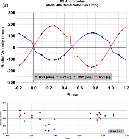
Figure 1. (a) The radial velocity data (obs) obtained by Mellergaard Amby (2011) and Model 40b computed radial velocities (c) described in the text. The data of the hotter and more massive component are represented by filled squares, those of the cooler secondary star by filled circles, and the computed curves are depicted in blue and red, respectively. The kinks in the computed curves at conjunctions for the star in eclipse are due to the McLaughlin–Rossiter effect, which the WD program simulates, along with proximity effects. Residuals in units of 100 km s−1 are shown in the bottom panel. (b) The Model 40a fittings of the IC and RC, RADS and non-RADS photometry passband data. The IC and RC data are represented by filled diamonds in the upper and middle panel sets, respectively, with the RADS data on the left and the non-RADS data on the right. In the combined data sets in the lower panels, IC and RC curves are on the left and right, respectively; the RADS data are shown as crosses, the non-RADS data as unfilled diamonds. In the lowest panel, IC and RC residuals are shown as gray and red filled squares for RADS and circles for non-RADS data, respectively. (c) The Model 40b fittings of the V and B RADS and non-RADS photometry passband data. The V and B data are represented by diamonds in the upper two panel sets, the RADS data on the left and the non-RADS data on the right. In the combined third panel sets, V and B are on the left and right, respectively; the RADS data are shown as crosses, the non-RADS data as filled diamonds. In the lowest two panels, V and B residuals are shown as squares for RADS and diamonds for non-RADS data.
Download figure:
Standard image High-resolution image
Figure 2. The fitting to a parabola of the square of the input average residual from a grid search for the visual extinction, AV, of two-passband RADS-weighted runs of a 2T, third-light model. The minimum of that fitting, at AV = 0.1059, is indicated.
Download figure:
Standard image High-resolution imageTable 2. DS Andromedae Model 40 Adjusted Parametersa
| Model | 40a | 40b | 40c | 40d | 40e | 40f | 40'' | 40 |
|---|---|---|---|---|---|---|---|---|
| (Passbands)/ | (IcRc) | (VB) | (IcV) | (IcB) | (RcV) | (RcB) | (IcRcVB) |
 IcRcVB IcRcVB 
|
| Parameter | (eight bands) | (columns 2–7) | ||||||
| a | 5.941 | 5.923 | 5.945 | 5.918 | 5.938 | 5.910 | 5.877 | 5.930 |
| (RSun) | 0.036 | 0.035 | 0.034 | 0.037 | 0.034 | 0.037 | 0.039 | 0.006[0.015] |
| Vsys | +8.09 | +8.21 | +8.16 | +8.09 | +8.17 | +8.08 | +8.05 | +8.13 |
| (km s−1) | 0.56 | 0.63 | 0.58 | 0.57 | 0.59 | 0.58 | 0.60 | 0.02[0.24] |
| i | 89.47 | 88.86 | 89.01 | 88.71 | 89.56 | 89.81 | 89.44 | 89.35 |
| (deg) | 0.53 | 0.37 | 0.46 | 0.45 | 0.40 | 0.26 | 0.28 | 0.19[0.16] |
| T1 | 6884 | 7052 | 7014 | 7027 | 7162 | 7091 | 7059 | 7056 |
| (K) | 81 | 30 | 38 | 21 | 51 | 20 | 16 | 21[12] |
| T2 | 5752 | 6019 | 5983 | 5894 | 6087 | 5968 | 5987 | 5971 |
| (K) | 66 | 31 | 38 | 36 | 46 | 29 | 21 | 33[15] |
| Ω1 | 3.566 | 3.577 | 3.580 | 3.572 | 3.579 | 3.567 | 3.551 | 3.574 |
| 0.017 | 0.015 | 0.016 | 0.017 | 0.015 | 0.017 | 0.016 | 0.003[0.007] | |
| Ω2 | 4.274 | 4.321 | 4.304 | 4.319 | 4.314 | 4.271 | 4.238 | 4.302 |
| 0.068 | 0.051 | 0.063 | 0.072 | 0.054 | 0.059 | 0.052 | 0.009[0.024] | |
| q | 0.659 | 0.656 | 0.663 | 0.653 | 0.661 | 0.650 | 0.642 | 0.657 |
| 0.009 | 0.009 | 0.009 | 0.010 | 0.009 | 0.010 | 0.010 | 0.002[0.004] | |
| t0 | .403315 | .401926 | .402397 | .403477 | .402252 | .403277 | .402898 | .402813 |
| HJD | .001093 | .001232 | .001150 | .001119 | .001149 | .001112 | .001130 | .000265 |
| fractn | [.000465] | |||||||
| P(day) | 188143 | 189627 | 189052 | 188180 | 189142 | 188299 | 188576 | 188697 |
| 1.0105+ | 001137 | 001301 | 001206 | 001171 | 001211 | 001171 | 001196 | 000247[000488] |
| log d | 2.666 | 2.675 | 2.676 | 2.668 | 2.692 | 2.682 | 2.675 | 2.678 |
| (pc) | 0.011 | 0.006 | 0.008 | 0.008 | 0.008 | 0.006 | 0.004 | 0.004[0.003] |
| (m0 – M) | 8.329 | 8.373 | 8.380 | 8.338 | 8.462 | 8.412 | 8.376 | 8.390 |
| (mag) | 0.056 | 0.030 | 0.040 | 0.042 | 0.039 | 0.028 | 0.020 | 0.018[0.015] |
| ℓ3(Ic)R | 0.113 | ⋯ | 0.100 | 0.086 | ⋯ | ⋯ | 0.103 | 0.100 |
| (ℓ1+2+3) | 0.021 | ⋯ | 0.019 | 0.023 | ⋯ | ⋯ | 0.008 | 0.007[0.012] |
| ℓ3(Rc)R | 0.112 | ⋯ | ⋯ | ⋯ | 0.099 | 0.101 | 0.090 | 0.103 |
| (ℓ1+2+3) | 0.019 | ⋯ | ⋯ | ⋯ | 0.015 | 0.013 | 0.007 | 0.004[0.009] |
| ℓ3(V)R | ⋯ | 0.099 | 0.112 | ⋯ | 0.106 | ⋯ | 0.105 | 0.103 |
| (ℓ1+2+3) | ⋯ | 0.010 | 0.018 | ⋯ | 0.014 | ⋯ | 0.006 | 0.004[0.007] |
| ℓ3(B)R | ⋯ | 0.097 | ⋯ | 0.097 | ⋯ | 0.109 | 0.104 | 0.101 |
| (ℓ1+2+3) | ⋯ | 0.009 | ⋯ | 0.022 | ⋯ | 0.012 | 0.006 | 0.004[0.007] |
| ℓ3(Ic)n | 0.110 | ⋯ | 0.097 | 0.083 | ⋯ | ⋯ | 0.097 | 0.098 |
| (ℓ1+2+3) | 0.021 | ⋯ | 0.019 | 0.023 | ⋯ | ⋯ | 0.007 | 0.008[0.012] |
| ℓ3(Rc)n | 0.116 | ⋯ | ⋯ | ⋯ | 0.100 | 0.104 | 0.092 | 0.105 |
| (ℓ1+2+3) | 0.020 | ⋯ | ⋯ | ⋯ | 0.015 | 0.013 | 0.007 | 0.004[0.009] |
| ℓ3(V)n | ⋯ | .0.084 | 0.098 | ⋯ | 0.092 | ⋯ | 0.092 | 0.088 |
| (ℓ1+2+3) | ⋯ | 0.009 | 0.018 | ⋯ | 0.015 | ⋯ | 0.006 | 0.004[0.007] |
| ℓ3(B)n | ⋯ | 0.083 | ⋯ | 0.086 | ⋯ | 0.097 | 0.090 | 0.088 |
| (ℓ1+2+3) | ⋯ | 0.009 | ⋯ | 0.022 | ⋯ | 0.012 | 0.006 | 0.005[0.007] |
 × 10−8 × 10⁻⁸ |
2.7720 | 4.0207 | 3.3160 | 3.8900 | 3.2863 | 3.8837 | 3.5380 | 3.5281 |
Note.
aThe Model 40 entries in the last column are the weighted means of Models 40a through 40f; the m.s.e.'s of the means are below (followed by those from the combination of parameter s.d.'s, in brackets). They indicate only the dispersion among the runs and contain no systematic error estimates (see Sections 3.4 and 4). The third-light parameter values have been normalized by the total system light (at phases 0.25 and 0.75). The first four ℓ3(pb) rows are the RADS bands values, the last four are non-RADS bands values. The weighted means of both bands are IC: 0.099(1); RC: 0.104(1); V: 0.095(7); B: 0.094(7).Download table as: ASCIITypeset image
3.5. Spot Models
Spots were introduced to model the largest RV1 residuals in Figure 1(a) as well as the slight light-curve enhancements in Figures 1(b) and (c) and described in Section 3.4. In spot modeling, it is typical to place cool spots on the cooler star, but in this system, that model did not converge. Thus, to improve the fitting of the RV1 data in the first quadrature by weighting some disk grid elements to simulate a velocity distortion, a cool spot was placed on star 1 (in Models 42A, 42B, and 43r), and for this spot, start and stop times were set for the RV data interval only. For the most noticeable enhancement in maximum I (that following the primary minimum) seen in the IC light curve (Figure 1(b)), a hot spot was placed on star 1 (Models 42–50). Usually all four parameters of a spot were adjusted. In two-spot models, usually only one parameter was adjusted per spot, and the parameters cyclically adjusted until consistency was obtained. The moments of onset and end of the spots were varied prior to runs to test the effects of spots on each of the observing segments, but no improvements were found. The latter spot parameters were relatively poorly determined, and the RV fitting not noticeably improved, so the two-spot models were abandoned. In Model 51, a hot spot was placed on star 2's opposite hemisphere. In Model 52, a single cool spot was placed on star 1 but on the opposite hemisphere from that assumed for models with a hot spot on star 1. Star 2 could be expected to have a deeper convection zone, if present, than star 1, but model runs with a cool spot on star 2 failed to converge. Third light was removed for Models 47 and 48 to see if spots alone could provide a better fit. None of the spot models, with or without third light, improved the fit significantly. The mean parameters of this group of models are listed in Column 7 of Table 3; note the large  value. A pdf of the full spreadsheet Table 3 in the repository shows the spot parameters of all models. The adopted model does not include spots.
Table 3. DS Andromedae Adjusted Parameters Summarya
| Group/ | 2-T | ARV | Av = .1 | Solar | Third | Spot | Non-sp | R/nR | Wtd Means |
|---|---|---|---|---|---|---|---|---|---|
| Parameter | Models | Models | Models | [M/H] | Light | Models | Models | Cases | |
| a | 5.862 | 5.925 | 5.933 | 5.933 | 5.937 | 5.948 | 5.934 | 5.917 | 5.940 |
| (RSun) | 0.015 | 0.006 | 0.007 | 0.007 | 0.005 | 0.003 | 0.007 | 0.011 | 0.004 |
| Vsys | +7.34 | +8.13 | +8.14 | +8.14 | +8.15 | +8.16 | +8.15 | +8.11 | +8.15 |
| (km s−1) | 0.22 | 0.01 | 0.01 | 0.01 | 0.01 | 0.01 | 0.02 | 0.02 | 0.01 |
| i | 87.43 | 88.49 | 88.92 | 88.87 | 89.55 | 89.08 | 89.23 | 89.23 | 89.32 |
| (deg) | 0.30 | 0.26 | 0.24 | 0.25 | 0.07 | 0.33 | 0.22 | 0.08 | 0.17 |
| T1 | 7059 | 7063 | 7067 | 7064 | 7070 | 7053 | 7071 | 7046 | 7064 |
| (K) | 6 | 8 | 9 | 9 | 8 | 11 | 12 | 21 | 3 |
| T2 | 5931 | 5929 | 5928 | 5921 | 5962 | 5946 | 5926 | 5954 | 5950 |
| (K) | 13 | 17 | 23 | 25 | 08 | 14 | 34 | 18 | 6 |
| Ω1 | 3.542 | 3.593 | 3.595 | 3.595 | 3.592 | 3.608 | 3.587 | 3.575 | 3.595 |
| 0.012 | 0.004 | 0.004 | 0.005 | 0.006 | 0.005 | 0.005 | 0.012 | 0.005 | |
| Ω2 | 4.252 | 4.355 | 4.334 | 4.338 | 4.286 | 4.352 | 4.299 | 4.282 | 4.305 |
| 0.034 | 0.017 | 0.018 | 0.019 | 0.008 | 0.033 | 0.014 | 0.015 | 0.010 | |
| q | 0.624 | 0.656 | 0.658 | 0.658 | 0.659 | 0.656 | 0.658 | 0.654 | 0.657 |
| 0.008 | 0.002 | 0.002 | 0.002 | 0.002 | 0.001 | 0.002 | 0.003 | 0.001 | |
| log d | 2.657 | 2.664 | 2.670 | 2.669 | 2.690 | 2.670 | 2.677 | 2.675 | 2.673 |
| (pc) | 0.004 | 0.004 | 0.004 | 0.005 | 0.008 | 0.009 | 0.003 | 0.004 | 0.003 |
| t0 | .399622 | .402897 | .402789 | .402793 | .402663 | .402679 | .402751 | .402719 | .402756 |
| 2436142+ | .001099 | .000071 | .000071 | .000071 | .000058 | .000098 | .000070 | .000083 | .000056 |
| P (day) | 92165 | 88605 | 88693 | 88703 | 88776 | 88791 | 88733 | 88711 | 88729 |
| 1.010514+ | 1189 | 58 | 57 | 57 | 33 | 60 | 62 | 61 | 40 |
 × 10−8 × 10⁻⁸ |
7.907 | 9.469 | 8.858 | 8.789 | 9.337 | 10.511 | 8.623 | 5.198 | 8.587 |
Note.
aBelow each group mean is the m.s.e. of the mean, signifying mainly the dispersion among models of that group but containing no estimate of the significant systematic error. Column 10 shows the grand means of the weighted means of columns 3 through 9, and the same qualification for its m.s.e.'s applies. The square root of the sum of the inverse squares of the m.s.e.'s of the means is usually smaller; for parameters a to log d these are, respectively, a, 0.002; Vsys, 0.004; i, 0.05; T1, 4; T2, 6; Ω1, 0.002; Ω2, 0.005; q, 0.001, log d, 0.002, t0, .000028; and P, 19 × 10−8. A pdf copy of the complete spreadsheet version of Table 3 can be found in the Zenodo repository 10.5281/zenodo.2553042. See the text for details.Download table as: ASCIITypeset image
3.6. Passband Absolute Calibration Constants and Metallicity Tests
The DDE algorithm deals with absolute units and requires a calibration constant (CALIB in Wilson & Van Hamme 2013) for each passband. The calibration constants are used when log d is adjusted. The constants for V and B used for all previous modeling were 0.36949 for V and 0.62350 for B (Wilson 2015, private communication), 0.122 for IC and 0.225 for RC (Bessell 1979), all in units of erg s−1 cm−3. The effects of changing both metallicity and passband calibration constants were explored in Models 28C and 28D. AV = 0.1059 (see Sections 3.2 and 3.4, and Figure 2) was adopted for these trials. The test series made use of only two passbands, ensuring strict adherence to the T–d theorem (Section 3.1). The designations, calibration constants, and the sources from which they were derived were taken from Wilson & Van Hamme (2013, Table 3, reproduced in the detailed Section 3, in the repository). For each of the listed models, runs were made for each of the three metallicities −0.1, 0, 1, and +0.1, signified by suffixes a, b, and c, respectively, in Tables 4 and 5. The last two columns of Table 4 contain  means for the calibration set, i.e., averaged across the metallicities, and the m.s.e. of the means. The mean residuals of the three metallicity runs for each calibration constant are not significantly different. There is no significant difference in
  between the runs with the R. E. Wilson (2015, private communication) and the Wilson et al. (2010) calibration constants, but those of the former are consistently smaller. Those for the other pairs of calibration constants are significantly larger.
Table 4. Models 28Cn and 28Dn Metallicity and Calibration Constant Trial Resultsa
| Model | [M/H] |
 × 10−8 × 10⁻⁸ |
Mean cal n  × 10−8 × 10⁻⁸ |
eMean × 10−8 |
|---|---|---|---|---|
| 28C1a | −0.1 | 4.71649 | ||
| 28C1b | 0.0 | 4.71141 | 4.70260 | 0.01145 |
| 28C1c | +0.1 | 4.67989 | ||
| 28C2a | −0.1 | 5.18844 | ||
| 28C2b | 0.0 | 5.20415 | 5.20268 | 0.00784 |
| 28C2c | +0.1 | 5.21546 | ||
| 28C3a | −0.1 | 4.98328 | ||
| 28C3b | 0.0 | 4.99198 | 4.98632 | 0.00283 |
| 28C3c | +0.1 | 4.98370 | ||
| 28C4a | −0.1 | 4.76459 | ||
| 28C4b | 0.0 | 4.77593 | 4.76320 | 0.00779 |
| 28C4c | +0.1 | 4.74907 | ||
| 28C5a | −0.1 | 4.73450 | ||
| 28C5b | 0.0 | 4.73586 | 4.72445 | 0.01073 |
| 28C5c | +0.1 | 4.70300 | ||
| 28D1a | −0.1 | 2.98538 | ||
| 28D1b | 0.0 | 2.98791 | 2.99006 | 0.00349 |
| 28D1c | +0.1 | 2.99689 | ||
| 28D2a | −0.1 | 2.87757 | ||
| 28D2b | 0.0 | 2.87112 | 2.87095 | 0.00387 |
| 28D2c | +0.1 | 2.86416 | ||
 runs runs |
0.0 | ⋯ | 4.88387 | 0.09422 |
 runs runs |
0.0 | ⋯ | 2.92951 | 0.08258 |
Note.
aColumns 4 and 5 show the mean residuals and their uncertainties for the three metallicity models (suffixes a, b, and c, respectively) of each calibration constant. The mean residuals for the Model 28Ca,c and 28Da,c runs are 4.87746(9138), 4.86622(10268) × 10−8; and 2.93146(7623), 2.93052(9385) × 10−8, respectively.Download table as: ASCIITypeset image
Table 5. DS Andromedae [M/H] and Calibration Test Models 28Cn,Dn Adjusted Parameter Meansa
| Model/ | 28C1 | 28C2 | 28C3 | 28C4 | 28C5 | 28D1 | 28D2 | [M/H] | [M/H] | [M/H] |
|---|---|---|---|---|---|---|---|---|---|---|
| Parameter | −0.1 | +0.0 | +0.1 | |||||||
 b
b
|
 b
b
|
 b
b
|
||||||||
| a | 5.956 | 5.956 | 5.958 | 5.956 | 5.957 | 5.939 | 5.944 | 5.956 | 5.957 | 5.957 |
| (RSun) | 0.002 | 0.001 | 0.001 | 0.001 | 0.000 | 0.002 | 0.002 | 0.002 | 0.001 | 0.002 |
| Vsys | +8.35 | +8.35 | +8.37 | +8.36 | +8.34 | +8.07 | +8.10 | +8.35 | +8.35 | +8.37 |
| (km s−1) | 0.01 | 0.00 | 0.01 | 0.02 | 0.06 | 0.01 | 0.01 | 0.00 | 0.01 | 0.01 |
| i | 89.46 | 89.78 | 89.42 | 89.12 | 89.15 | 88.93 | 89.09 | 89.88 | 89.11 | 89.27 |
| (deg) | 0.10 | 0.19 | 0.25 | 0.33 | 0.10 | 0.06 | 0.20 | 0.10 | 0.10 | 0.24 |
| T1 | 7052 | 7510 | 7539 | 7327 | 7088 | 6817 | 7275 | 7318 | 7287 | 7305 |
| (K) | 13 | 13 | 14 | 74 | 13 | 6 | 14 | 114 | 100 | 105 |
| T2 | 5876 | 6210 | 6230 | 6079 | 5903 | 5731 | 6081 | 6061 | 6039 | 6080 |
| (K) | 24 | 10 | 10 | 52 | 24 | 8 | 3 | 88 | 77 | 68 |
| Ω1 | 3.570 | 3.569 | 3.575 | 3.567 | 3.570 | 3.569 | 3.568 | 3.572 | 3.571 | 3.567 |
| 0.002 | 0.001 | 0.001 | 0.003 | 0.001 | 0.001 | 0.002 | 0.001 | 0.002 | 0.002 | |
| Ω2 | 4.289 | 4.271 | 4.288 | 4.286 | 4.295 | 4.285 | 4.281 | 4.279 | 4.286 | 4.293 |
| 0.005 | 0.003 | 0.005 | 0.005 | 0.007 | 0.002 | 0.004 | 0.002 | 0.004 | 0.008 | |
| q | 0.664 | 0.665 | 0.666 | 0.665 | 0.662 | 0.658 | 0.663 | 0.665 | 0.664 | 0.663 |
| (M2/M1) | 0.001 | 0.000 | 0.001 | 0.000 | 0.002 | 0.001 | 0.002 | 0.000 | 0.001 | 0.002 |
| t0 | .4014 | .4013 | .4013 | .4013 | .4015 | .4033 | .4032 | .4014 | .4014 | .4013 |
| HJDfr. | .0001 | .0000 | .0000 | .0001 | .0001 | .0000 | .0000 | .0000 | .0000 | .0001 |
| P (day) | 19025 | 19031 | 19035 | 19039 | 19018 | 18813 | 18822 | 19079 | 19025 | 19037 |
| 1.0105+ | 00005 | 00002 | 00003 | 00013 | 00006 | 00002 | 00002 | 00002 | 00004 | 00011 |
| log d | 2.681 | 2.733 | 2.746 | 2.706 | 2.685 | 2.658 | 2.715 | 2.706 | 2.710 | 2.715 |
| (pc) | 0.003 | 0.003 | 0.003 | 0.001 | 0.002 | 0.002 | 0.000 | 0.013 | 0.012 | 0.013 |
Notes.
aMean standard errors are given for each model below the parameters. The inverse square root of the sums of the inverse squares of the individual-run errors is usually similar but sometimes may exceed the m.s.e. of the mean. The robustness of most parameters is striking but T1,2 are particularly sensitive to the choice of calibration constant, as the m.s.e.'s of their means indicate. bThe mean parameters for the same [M/H] in columns 9–11 are for 28C models only.Download table as: ASCIITypeset image
Some VB runs yielded T1,2 that were too high for the early-F observed spectral type of the system, so their use here can be rejected as unphysical, further supporting the selection of the R. E. Wilson (2015, private communication) V and B calibration constants. For the IC and RC passbands, the constants of Bessell et al. (1998) produced consistently smaller mean residuals compared with the Bessell (1979) calibration constants, but yielded temperatures that were, again, too high. The resulting high temperatures skew the radiative parameter means across the models as can be seen in the last three columns of Table 5. The m.s.e. of T1,2 are ∼100 and 80 K, and those of log d ∼ 0.012, setting upper limits for systematic error due to calibration constant selection.
3.7. Detailed Reflection Model Tests
Suspecting that the secondary star may exhibit a large reflection effect, due to the proximity in this system of a larger and hotter companion, we ran the template model 28C1b with enhanced reflection (Wilson et al. 2010), mref = 3, keeping the number of reflections at (nref =) 2. This model (28C1bR) showed significant changes to some of the parameters, but the overall fit was no better. The mean residual for this model was 4.758 × 10⁻⁸, whereas  = 4.711 × 10⁻⁸ for Model 28C1b. As the temperature of star 2 had now slipped below that of the Sun (in WD 2013, TSun = 5779 K is assumed), Model 28C1bR was rerun with convective envelope coefficients A2 = 0.500 and g2 = 0.32, and designated Model 28C1bRC. This did not improve the fitting (
 = 4.964 × 10⁻⁸). The insertion of nonsynchronous rotation factors did not make significant changes to the parameters and to their uncertainties: we set F1 = Porb/Prot,1 = 1.047 and F2 = Porb/Prot,2 = 1.006, appropriate for v1 = 103 and v2 = 63 km s−1, slightly off synchronism. Running this last model with an additional reflection, nref = 3, again produced no significant changes and only a slight improvement in
  . The means of the adjusted parameters of two trials are included in Table 6 (column 2).
Table 6. DS Andromedae Adjusted Parameters of Detailed Reflection and Semidetached Modelsa
| Modela/ | 28...R3 | 53a | 53a1 | 53a2 | 53b | 53b1 | 53b2 |
|---|---|---|---|---|---|---|---|
| Parameter | |||||||
| a (RSun) | 5.947 | 6.305 | 6.300 | 6.302 | 6.424 | 6.016 | 5.968 |
| 0.030 | 0.042 | 0.042 | 0.042 | 0.048 | 0.029 | 0.050 | |
| Vsys | +8.33 | +8.18 | +8.17 | +8.17 | +7.62 | +8.08 | +8.16 |
| (km s−1) | 0.46 | 0.42 | 0.42 | 0.42 | 0.72 | 0.52 | 0.52 |
| i | 86.84 | 72.60 | 72.74 | 72.74 | 73.49 | 85.09 | 89.70 |
| (deg) | 0.18 | 0.10 | 0.24 | 0.24 | 0.13 | 0.47 | 1.10 |
| T1 | 7043 | 7347 | 7116 | 7116 | 7923 | 7386 | 7337 |
| (K) | 23 | 11 | 43 | 43 | 27 | 79 | 80 |
| T2 | 5712 | 5908 | 5722 | 5722 | 6657 | 6232 | 6388 |
| (K) | 21 | 23 | 38 | 38 | 22 | 64 | 67 |
| Ω1 | 3.559 | 3.927 | 3.940 | 3.939 | 4.611 | 5.266 | 5.086 |
| 0.011 | 0.030 | 0.033 | 0.034 | 0.049 | 0.082 | 0.039 | |
| Ω2b | 4.437 | 3.205 | 3.206 | 3.205 | 3.135 | 3.135 | 3.209 |
| 0.034 | ⋯ | ⋯ | ⋯ | ⋯ | ⋯ | ⋯ | |
| q | 0.676 | 0.677 | 0.677 | 0.677 | 0.722 | 0.680 | 0.681 |
| (M2/M1) | 0.006 | 0.008 | 0.008 | 0.008 | 0.010 | 0.006 | 0.009 |
| t0 | .3939 | .3957 | .3957 | .3956 | .4043 | .4024 | .3975 |
| HJDfr.c | 0012 | .0013 | .0013 | .0013 | .0014 | .0013 | .0014 |
| P (day)1.0105+ | 19829 | 19627 | 19627 | 19631 | 18717 | 18916 | 19425 |
| 00128 | 00130 | 00131 | 00130 | 00148 | 00151 | 00151 | |
| log d | 2.667 | 2.723 | 2.692 | 2.682 | 2.782 | 2.750 | 2.764 |
| (pc) | 0.005 | 0.003 | 0.008 | 0.008 | 0.005 | 0.010 | 0.008 |
Notes.
aModel 28...R3 results are the means of the small and large grid size detached Model 28C1bRCR3 runs. The error below each parameter is the inverse square root of the sum of inverse squares of the two s.d.'s; this error exceeds the m.s.e. of the mean in every case. Columns 3–8 are individual-run results from Mode 5 semidetached models in the "53a" (VB) and "53b" (ICRC) series, and their s.d.'s are given below. See Section 3.8 for further details. bOmega2 values are unadjusted in mode 5. cHJDfr = fraction of the heliocentric Julian date.Download table as: ASCIITypeset image
3.8. Semidetached Test models
Star 1 had been consistently the larger component in all detached model run results. Thus, we initially tested semidetached (SD) models in mode 4, in which the potential of Star 1 is not adjusted but internally set to that of its inner Lagrangian surface; they failed to converge.
After the runs described in Sections 3.1–3.7 were completed, we sought a model that would not only provide better fittings to the data but would also help with the secondary luminosity problem, to be discussed in Section 6. We used a template with detailed reflection, convective envelope parameters for A2 and g2 and ran tests in mode 5, in which Ω1 is adjusted while Ω2 is internally computed by the program. After many runs, convergence was achieved with  fixed at zero: Model 53_SD5a, the parameters of which are listed in column 3 of Table 6 under header "53a." The errors, beneath the parameters, are their standard deviations, from the DC output files. With the ICRC suite and
  fixed at 0, convergence was achieved after 15 runs. This is Model 53_SD5b (header "53b" in Table 6). The two sets of SD models differ significantly from each other and from the detached solutions. To check the robustness of the SD solutions, third light was again adjusted and after four runs, convergence was achieved for the ICRC passband suite, Model 53_SD5b1 (header "53b1" in Table 6). For the VB passband suite, convergence was also found, Model 53_SD5a1 (header "53a1" in Table 6), but in this case, the
  value was not significant and the
  value only marginally so. In all the SD5 models studied thus far, T1,2 were larger than those in the detached models, but had been run with convective envelope parameters A2 and g2 Setting both to 1.00, appropriate for radiative envelopes (leaving aside the issue of the appropriateness of such an envelope for a lobe-filling star), we obtained convergence for the ICRC passband suite in the next run; this is Model 53_SD5b2 ("53b2" in the Table 6 header). No convergence was found for the VB passband suite for the radiative envelope case. We had previously found that restricting the range of phases around quadrature from 0.10P to 0.06P for the calculation of the standard errors at maximum light improved
  for VB suite runs. ICRC suite runs showed no such improvement, so the range was left at 0.1P. Model 53_SD5a1 rerun with the range reset to 0.10P is Model 53_SD5a2 (Table 6 header "53a2"). The results are not significantly different. Although parameter errors may differ, in all cases,
  for the converged semidetached models exceeded those of Model 40 detached models. These results confirm the impression given by the rounded, transit-like primary minimum and the occultation-like secondary minimum already seen in the SM88 plots. We therefore favor the detached mode models.
3.9. Period Variation Trials
Given the presence of third light, Models 28C1b and 28D1b were rerun with the period variation, or P-dot (for dP/dt), parameter adjusted along with all the other parameters. The two sets of trials show significant dP/dt terms, but one only marginally, and they disagree. Only the period and epoch, among the other parameters, were significantly changed. For Model 28C1bP, involving VB passbands,  = 4.462 × 10⁻⁸ and critical parameters t0 = 2436142.2819(183), P0 = 1.01053838(295), and dP/dt = −1.393 (211) × 10−9 days/day. With detailed reflection, nref = 3, Model 28C1bPR yielded
  = 4.481 × 10⁻⁸, t0 =2436142.2798(185), P0 = 1.01053864(299), and dP/dt =−1.405(214) × 10−9. For Model 28D1bPR, with ICRC passbands,
  = 2.879 × 10⁻⁸, t0 = 2436142.4493(204), P0 = 1.01051138(329), and dP/dt = +5.330(2356) × 10−9. The results for the VB and ICRC suites are significantly different, casting doubt on the reality of the dP/dt term and making determination of parameters of any third body a matter for future investigation. A recent major O − C study is not supportive: an examination of all the times of minimum over the interval 1932 to 2015 by R. H. Nelson (2018, private communication; data available at http://www.aavso.org/bob-nelsons-o-c-files). With weightings of 0.1 applied to visual and photographic data and 1 for photoelectric and CCD times of minima, he found a marginally significant but very small, quadratic term, corresponding to dP/dt = +2.715(1151) × 10−11 day/day.
3.10. Effects of U Data Inclusion
Modeling was conducted in two stages. All five passbands as well as the two RV bands were run with L1, but not log d, adjusted in a Model 41 template file. The final converged values of the parameters were then used as starting parameters for subsequent runs of suites of two-band photometric and the RV curves, namely Models 55a (ICRC), 55b (ICV), 55c (ICB), 55d (ICU), 55e (RCV), 55f (RCB), 55g (RCU), 55h (VB), 55i (VU), and 55j (BU), in which the passband luminosities were not adjusted but log d was. The U bands were run with calibration constant 0.4221 (R. E. Wilson 2015, private communication). The weighted means of the adjusted and absolute parameters define Model 55. Excluding Models 55e and 55j, with parameters T1,2 and ℓ3, which exceeded Chauvenet's criterion, we define Model 55'. Its  exceeded that of Model 40 but the parameters agree within errors. We conclude that the exclusion of the U data for the bulk of the trials has had minimal impact on the adjusted parameters, and the increased uncertainty in many parameters when U data are included justifies their exclusion from the bulk of the modeling trials. Still, the exercise provided U curve parameters. The relative U passband luminosity [L1/(L1+L2)]U = 0.912(3), and(ℓ3/ℓ1+2+3)U = 0.122(9), where the errors are the m.s.e.'s of the means. For further modeling details, see the document "DS ANDROMEDAE CURVES ANALYSES: EXTENDED DISCUSSION VERSION" with references and a pdf copy of the expanded online spreadsheet version of Table 3 in Zenodo 10.5281/zenodo.2553042.
4. Summary of Adjusted Parameter Results
Adjusted parameters obtained from runs of limited numbers of curves differ among themselves and, in the absence of compelling preferences, need to be averaged. Typically, to satisfy the T–d theorem, if T1,2 and log d are adjusted, only two passbands can be run simultaneously with the RV curves to avoid over- or underconditioning; hence, with four passbands, six runs are required for the six passband pairings, in order to use all available data. Table 2 contains the adjusted parameters from Models 40a–f (the converged DC runs with the smallest mean residuals) and the means of those runs (Model 40). It also lists parameters from a run in which all four ICRCVB passbands are included (Model 40''); this run had the next smallest mean residual, 3.528 × 10⁻⁸, after the Model 40a–f runs. There are no significant differences in the adjusted parameters between Models 40 and 40''.
Table 3 contains the summary of the averaged adjusted parameters of the models described in Sections 3.1–3.4 and the quantities derived from them. The 10th and last column contains the grand means—the weighted means of all model groups except the "2-T" model group of column 2, some of which include runs carried out with the SM88 RVs. Column 8, the nonspot models group, is a subset of Column 6. The models described in Sections 3.5–3.9 are not included in the group means in Table 3 for a variety of reasons. The SD models are excluded because they represent major changes to the structure of the binary and, like other tests such as the AV grid trials and those of the different calibration constants, involve only the VB or ICRC passband pairs along with RVs. An expanded pdf version of Table 3, entitled "DS_AND_PARAMETERS_Table_3 Adjusted Parameters Summary" with parameters of all detached models contributing to the means, the group means, and the grand means, is found within the Zenodo repository supplement package 10.5281/zenodo.2553042. The read-me file enclosed therein describes the documents included in the package, and the column headings for all tables.
A comparison of the grand means of Table 3 with those of Model 40 in Table 2 indicates significant agreement for all adjusted parameters except Ω1, for which the difference is still less than 3σ. Generally, the parameter means of a model, consisting of several runs with different suites of data, or of a group of different models, do not correspond to any single optimized fitting, but Model 40 mean parameters inserted into a Model 40'' template still produce convergence. For the purposes of this paper, therefore, we adopt the Model 40 parameters.
The parameter means of the runs, models, and groups of models are not fully independent in two ways. First, the model means for some parameters may be more dependent on one subset of input data than others. Second, models may appear in multiple groups, slightly biasing the group averages and the grand means. For each model's means, data from each passband contribute three times but the RV bands contribute six times. Some dynamical parameters are more dependent on the RVs than on the light curves (see, e.g., Kallrath & Milone 2009, p. 22), so their dispersion and the m.s.e.'s of their means will be smaller than those of other parameters. However, all curves are carefully weighted, so the bias is probably less than one might suppose. The results of the semidetached models in Table 6, run with the same suites of input data, demonstrate how the dynamical parameters, among others, can vary widely with model. Nevertheless, if the runs are not fully independent, it may be argued that a more robust type of error should be cited as well as the m.s.e. of the mean. The errors found by the WD damped least-squares engine are no less accurate than those of any similar engine, and the curve sigmas indicate that the run errors include the scatter in the data as well as the error of fit, so we need to address only the errors of the means statistic. The m.s.e. of the weighted mean (call it e1) is usually similar to the m.s.e. of the unweighted mean (e2), because of the similarities of the parameter standard deviations (s.d.'s); a third statistic (e3) is the m.s.e. computed from the inverse square root of the sum of the inverse squares of each parameter's standard deviation. As an illustration, these three types of errors computed for Model 40 for the listed adjusted parameters are, respectively,
For consistency, we have elected to report e1 for the means in Tables 2–5, 9, 10 and 13, for which there are parameter s.d.'s, or m.s.e.'s, and e2, for which there are not (see Section 5). In Table 6, we report e3 (which for these means is larger than e1 and e2) for all parameters of the detached Model 28B...R3, and the s.d.'s for the single-run, SD models. In Table 14, we report e1, systematic error, and e3 (in footnote c).
The e1 errors listed for model, group, and grand means are not necessarily indicative of the true precision in those quantities, but merely of the dispersion among the parameters being averaged. Systematic errors likely dominate in runs or model means, but potential sources of systematic error due to effects explicitly tested in the included models, such as the selection of interstellar extinction or metallicity, add scatter and thereby contribute to a limited extent to the error of the group and grand means. Even so, the errors in all runs and means likely do not include all possible sources of systematic error arising from wider and external causes. The differences among the run parameters with different suites of passbands, for example, between Model 40a (ICRC), and Model 40b (VB) in Table 2 and between Models 28C1 and 28D1 in Table 5, illustrate the dispersion arising from bandpass effects. The trials described in Section 3.6 suggest the uncertainty in the adopted calibration constants is an important contributor to systematic error. The m.s.e.'s in the last two columns of Table 5 suggest upper limits of 100 K for T1, ∼80 K for T2 and 0.012 in log d (13 pc in d) for systematic error from this source. Allowing for systematic error in the temperature scale of ±100 K, and adding by quadrature, the systematic uncertainties in T1 and T2 estimates are ±140 K and ±130 K, respectively. Estimates for those of other parameters come from differences among Models 40, 40'', and group, and grand means.
5. Absolute Parameters of the DS Andromedae System
Table 7 lists absolute parameters for Models 40a–f, 40'', and 40 from the LC routine: masses, M1,2, and radii R1,2, in solar units, bolometric magnitudes, MBol,1,2, and the log of the gravitational acceleration in cgs units, log g1,2. Table 7 also contains derived relative passband luminosities,  (λ)/[
(λ)/[ (λ) +
(λ) +  (λ)], computed from
  (λ) and
  (λ), LC-produced passband luminosities in solar units (not to be confused with the adjusted parameter
  ). The bolometric luminosities,
  and
and  in solar units, are computed directly from MBol1,2 and MBol,Sun (assumed to be 4.75). The Model 40 luminosities
  = 9.59(19) and
  = 1.77(5)
  compare satisfactorily with those computed from the MBol,1,2 means. The mean absolute parameters of groups of models are presented in Table 8. The grand means in column 10 are the weighted means of columns 3–9 of each row. The weighted means of the bolometric luminosities, given in the last two rows, are
  =9.59(1),
  = 1.77(2)
  , in agreement with those computed from the MBol,1,2 means and those found for Model 40. Although there are departures from sphericity of the stars (see Section 5.2), the bolometric luminosities can be computed from the mean effective temperatures taken from Table 3 and the mean effective radii from Table 8: 4πσ
 2
2 Teff
Teff 4 = 3.69(1) × 1027 and 6.86(5) × 1026 W, equivalent to 9.59(2) and 1.78(1)
  , for stars 1 and 2, respectively. In fact, the corresponding parameter means in the last columns of Tables 7 and 8 agree within ∼2σ, except for R1, for which the difference is 0.013(4) RSun, indicative of systematic error. Analogous to Table 3, there is an extended spreadsheet pdf version of Table 8, "DS_AND_PARAMETERS_Table_8_Absolute_Parameters_Summary," in the Zenodo package (10.5281/zenodo.2553042), which provides a full list of the averages of the absolute parameters and quantities derived from them of individual models, the means of groups of models, and the grand means. We now consider the broad question of the reliability of the absolute parameter means and their uncertainties.
Table 7. Model 40 Absolute Parameters Summarya
| Model | 40a | 40b | 40c | 40d | 40e | 40f | 40'' | 40abcdef |
|---|---|---|---|---|---|---|---|---|
| (pbs) | (IcRc) | (VB) | (IcV) | (IcB) | (RcV) | (RcB) | (IcRcVB) | (IcRcVB) |
| /Parameter | (8 bds) | Means | ||||||
| M1(MSun) | 1.664 | 1.651 | 1.663 | 1.650 | 1.658 | 1.645 | 1.626 | 1.655(3) ± 0.030 |
| M2(MSun) | 1.096 | 1.083 | 1.102 | 1.077 | 1.096 | 1.070 | 1.044 | 1.087(5) ± 0.040 |
| R1(RSun) | 2.098 | 2.080 | 2.091 | 2.080 | 2.088 | 2.079 | 2.073 | 2.086(3) ± 0.013 |
| R2(RSun) | 1.272 | 1.244 | 1.267 | 1.238 | 1.258 | 1.252 | 1.243 | 1.255(5) ± 0.012 |
| Mbol1 | 2.38 | 2.29 | 2.31 | 2.31 | 2.22 | 2.27 | 2.30 | 2.30(2) |
| Mbol2 | 4.25 | 4.10 | 4.09 | 4.20 | 4.02 | 4.12 | 4.12 | 4.13(3) |
| log g1 | 4.02 | 4.02 | 4.02 | 4.02 | 4.02 | 4.02 | 4.02 | 4.02(0) |
| log g2 | 4.27 | 4.28 | 4.27 | 4.28 | 4.28 | 4.27 | 4.27 | 4.28(1) |
 (Ic)/( (Ic)/( ) ) |
0.826 | ⋯ | 0.815 | 0.828 | ⋯ | ⋯ | 0.820 | 0.823(4) |
 (Rc)/( (Rc)/( ) ) |
0.842 | ⋯ | ⋯ | ⋯ | 0.832 | 0.838 | 0.835 | 0.837(3) |
 (V)/( (V)/( ) ) |
⋯ | 0.848 | 0.845 | ⋯ | 0.848 | ⋯ | 0.851 | 0.847(1) |
 (B/( (B/( ) ) |
⋯ | 0.876 | ⋯ | 0.888 | ⋯ | 0.883 | 0.879 | 0.882(4) |
 / /
|
8.872 | 9.638 | 9.462 | 9.462 | 10.280 | 9.817 | 9.550 | 9.59(19) |
 / /
|
1.585 | 1.820 | 1.837 | 1.660 | 1.959 | 1.786 | 1.786 | 1.77(5) |
Note.
aAbsolute parameters for two-passband runs (detached Models 40a–f), a four-passband run with RADS and non-RADS data separated for a total of eight bands (Model 40''), and the means of the two-passband runs, Model 40, in column 9. The m.s.e.'s of the means follow in parentheses and estimates of the systematic error for M1,2 and R1,2 are below. Note that the LC routine does not provide the standard errors in the absolute parameters, so the means are unweighted. Bolometric luminosity is computed from Mbol. Model 40 computed from Mbol means are:
  = 9.58(12),
  = 1.77(3). See Section 5 for further detail.
Download table as: ASCIITypeset image
Table 8. DS Andromedae Weighted Means Absolute and Auxiliary Parameters Summarya
| Model | 2-T | ARV | Av = .1 | Solar | Third Light | Spot | Non-sp | R/non-R | Wtd Means |
|---|---|---|---|---|---|---|---|---|---|
| Group/ | Models | Models | Models | [M/H] | Models | Models | Models | Cases | |
| Parameter | Models | ||||||||
| M1(MSun) | 1.624 | 1.646 | 1.653 | 1.651 | 1.659 | 1.664 | 1.657 | 1.648 | 1.660 |
| 0.006 | 0.005 | 0.005 | 0.005 | 0.003 | 0.002 | 0.003 | 0.006 | 0.002 | |
| M2(MSun) | 1.007 | 1.074 | 1.087 | 1.083 | 1.094 | 1.104 | 1.091 | 1.076 | 1.096 |
| 0.016 | 0.008 | 0.007 | 0.008 | 0.004 | 0.003 | 0.005 | 0.010 | 0.004 | |
| R1(RSun) | 2.055 | 2.065 | 2.070 | 2.068 | 2.076 | 2.070 | 2.077 | 2.077 | 2.073 |
| 0.004 | 0.004 | 0.003 | 0.004 | 0.003 | 0.004 | 0.003 | 0.006 | 0.002 | |
| R2(RSun) | 1.200 | 1.231 | 1.245 | 1.240 | 1.267 | 1.248 | 1.266 | 1.253 | 1.260 |
| 0.010 | 0.010 | 0.009 | 0.010 | 0.003 | 0.015 | 0.004 | 0.004 | 0.004 | |
| Mbol1 | 2.318 | 2.301 | 2.297 | 2.298 | 2.291 | 2.293 | 2.290 | 2.304 | 2.296 |
| 0.007 | 0.006 | 0.006 | 0.006 | 0.008 | 0.005 | 0.010 | 0.022 | 0.002 | |
| Mbol2 | 4.238 | 4.186 | 4.153 | 4.161 | 4.108 | 4.136 | 4.116 | 4.148 | 4.130 |
| 0.020 | 0.020 | 0.019 | 0.020 | 0.008 | 0.029 | 0.009 | 0.009 | 0.009 | |
| log g1 | 4.022 | 4.024 | 4.024 | 4.024 | 4.021 | 4.027 | 4.021 | 4.021 | 4.023 |
| 0.001 | 0.001 | 0.001 | 0.002 | 0.001 | 0.002 | 0.001 | 0.003 | 0.001 | |
| log g2 | 4.280 | 4.288 | 4.283 | 4.286 | 4.270 | 4.289 | 4.268 | 4.274 | 4.275 |
| 0.005 | 0.005 | 0.005 | 0.005 | 0.003 | 0.010 | 0.003 | 0.002 | 0.003 | |
 (IC) (IC) |
0.832 | 0.827 | 0.823 | 0.824 | 0.818 | 0.822 | 0.819 | 0.821 | 0.820 |
( + + )Ic )Ic |
0.002 | 0.002 | 0.002 | 0.002 | 0.001 | 0.003 | 0.001 | 0.002 | 0.001 |
 (RC) (RC) |
0.845 | 0.842 | 0.838 | 0.839 | 0.833 | 0.837 | 0.834 | 0.836 | 0.835 |
( + + )Rc )Rc |
0.002 | 0.002 | 0.002 | 0.002 | 0.001 | 0.003 | 0.001 | 0.002 | 0.001 |
 (V) (V) |
0.861 | 0.857 | 0.853 | 0.854 | 0.848 | 0.852 | 0.849 | 0.850 | 0.850 |
( + + )V )V |
0.002 | 0.002 | 0.002 | 0.002 | 0.001 | 0.003 | 0.001 | 0.002 | 0.001 |
 (B) (B) |
0.890 | 0.887 | 0.884 | 0.884 | 0.880 | 0.882 | 0.881 | 0.881 | 0.882 |
( + + )B )B |
0.002 | 0.002 | 0.002 | 0.002 | 0.001 | 0.002 | 0.001 | 0.002 | 0.001 |
 ( ( ) ) |
9.40 | 9.55 | 9.58 | 9.58 | 9.63 | 9.62 | 9.64 | 9.52 | 9.591 |
| 0.06 | 0.06 | 0.05 | 0.06 | 0.07 | 0.05 | 0.09 | 0.19 | 0.013 | |
 ( ( ) ) |
1.61 | 1.69 | 1.74 | 1.73 | 1.81 | 1.77 | 1.79 | 1.74 | 1.770 |
| 0.03 | 0.03 | 0.03 | 0.03 | 0.01 | 0.04 | 0.02 | 0.02 | 0.015 |
Note.
aMeans for models with fixed T1 are omitted. The m.s.e.'s below each mean are internal only; they include no systematic error. The relative passband luminosities were obtained from those in solar units computed in the LC routine of the WD program. are computed from Mbol1,2, except for Column 10, the "grand means," which are the weighted means of the groups means.
  computed from grand means
  Mbol1,2
 are
are  = 9.587(29) and
  = 1.770(12). Note the agreement with Model 40 means (Table 7). A pdf copy of the complete spreadsheet version of Table 8 can be found in the Zenodo repository, 10.5281/zenodo.2553042 .
Download table as: ASCIITypeset image
The absolute parameter uncertainties in any run are not provided by the LC program so the model averages from those runs are unweighted, unlike those from the adjusted parameter DC runs. The group means of both adjusted and absolute parameters are also unweighted means of the models of that group. Finally, the grand means of the group parameters are weighted group means. The caveats regarding the uncertainties of the adjusted parameter means discussed in Section 4 apply to those of the absolute parameters. The range of luminosity among Models 40a–f and 40'' in Table 7 provides evidence of systematic error due to passband effects: differences of more than 10% in some run parameters can be seen. The averages tend to smooth out these differences, which is their purpose, but the range of values provides a reminder that the m.s.e. is probabilistic, based on an expected single Gaussian distribution of error, and that it reports primarily the dispersion among assumedly independent individual model means. The accuracy of some of the absolute parameters can be addressed further, at least for some of the dynamical parameters, from the independent analyses of the RV data by Mellergaard Amby (2011; Th.M.A.) and G. Torres (G.T.). The results are summarized in Columns 2 and 3, respectively, of Table 9, where they are compared with those from Models 40a, 40b, 28C1b, and 40, and the grand means. K1,2 are the semi-amplitudes of the sine curves of stars 1 and 2 fitted to the data. No Rossiter–McLaughlin or proximity effects, visible in Figure 1(a) (having a small influence on the data nearest to conjunctions), were included in these analyses. The sigmas for each curve are shown at the bottom of Table 9. The Th.M.A. and G.T. results agree with the Model 40 results to within ∼2σ, the largest differences occurring in q and M1. Thus, the grand averaging process provides masses, radii, bolometric magnitudes, log g, temperature, passband luminosity ratios, and bolometric luminosities that are consistent with properties of the best individual model means but is still subject to additional sources of systematic error within the model groups and beyond, such as in the data bands, calibration constants, temperature scale, other assumed constants, and the scaling operations performed in LC. For this paper, we adopt the Model 40 parameters and use differences from Model 40'' and group and grand means for estimates of systematic uncertainties. Tables 5 and 10 reveal the effects of changing metallicity and calibration constants on the parameters. Table 10 lists the absolute and auxiliary parameters of the Model 28C and 28D tests for an array of calibration constants and three values of metallicity, all carried out with Av fixed at 0.1059. In these models, the largest scatter is seen in MBol,1,2, and the bolometric and passband luminosities; relative passband luminosities are not greatly affected.
Table 9. Dynamical Adjusted and Auxiliary Parameters
| Analysis/Parameter | Th.M.A.a | G.T.a | Mod. 40a | Mod. 40b | Mod. 28C1b | Mod. 40 | Grand Means | |
|---|---|---|---|---|---|---|---|---|
| a | 5.92b | 5.916b | 5.941 | 5.923 | 5.959 | 5.930 | 5.940 | |
| (RSun) | 0.10 | 0.025 | 0.036 | 0.035 | 0.033 | 0.006 | 0.004 | |
| Vsys | +8.44 | +8.18 | +8.09 | +8.21 | +8.34 | +8.13 | +8.15 | |
| (km s−1) | 0.60 | 0.52 | 0.56 | 0.63 | 0.63 | 0.02 | 0.01 | |
| K1 | 119.98 | 119.75 | ⋯ | ⋯ | ⋯ | ⋯ | ⋯ | |
| (km s−1) | 0.98 | 0.98 | ⋯ | ⋯ | ⋯ | ⋯ | ⋯ | |
| K2 | 176.55 | 176.36 | ⋯ | ⋯ | ⋯ | ⋯ | ⋯ | |
| (km s−1) | 0.98 | 0.77 | ⋯ | ⋯ | ⋯ | ⋯ | ⋯ | |
| M1 | 1.625c | 1.620c | 1.664 | 1.651 | 1.672 | 1.655 | 1.660 | |
| (MSun) | 0.018 | 0.019 | ⋯ | ⋯ | ⋯ | 0.003 | 0.002 | |
| M2 | 1.105c | 1.099c | 1.096 | 1.083 | 1.112 | 1.087 | 1.096 | |
| (MSun) | 0.019 | 0.017 | ⋯ | ⋯ | ⋯ | 0.005 | 0.004 | |
| q | 0.680 | 0.679 | 0.659 | 0.656 | 0.665 | 0.657 | 0.657 | |
| 0.007 | 0.006 | 0.009 | 0.009 | 0.008 | 0.002 | 0.001 | ||
| i | ⋯ | ⋯ | 89.47 | 88.86 | 89.49 | 89.35 | 89.32 | |
| (deg) | ⋯ | ⋯ | 0.53 | 0.37 | 0.46 | 0.19 | 0.17 | |
| σ(RV1) (km s−1) | 3.96 | 3.14 | 4.97 | 4.68 | 4.18 | 4.82(13) | ⋯ | |
| σ (RV2) (km s−1); | 2.52 | 2.45 | 2.03 | 2.35 | 2.43 | 2.14(5) | ⋯ | |
| σ(IC, R)d | ⋯ | ⋯ | 2.52 | ⋯ | ⋯ | 2.587(6) | ⋯ | |
| σ(IC, n)d | ⋯ | ⋯ | 1.26 | ⋯ | ⋯ | 1.250(4) | ⋯ | |
| σ(RC,R)d | ⋯ | ⋯ | 2.79 | ⋯ | ⋯ | 2.790(3) | ⋯ | |
| σ(RC,n)d | ⋯ | ⋯ | 1.12 | ⋯ | ⋯ | 1.114(4) | ⋯ | |
| σ(V, R)d | ⋯ | ⋯ | ⋯ | 4.48 | 1.56e | 4.483(8) | ⋯ | |
| σ(V, n)d | ⋯ | ⋯ | ⋯ | 1.32 | 1.316(3) | ⋯ | ||
| σ(B, R)d | ⋯ | ⋯ | ⋯ | 5.43 | 1.76e | 5.437(13) | ⋯ | |
| σ(B, n)d | ⋯ | ⋯ | ⋯ | 1.59 | 1.568(10) | ⋯ | ||
Notes.
aRV analyses: Th.M.A. = Th. Mellergaard Amby (2011), G.T. = G. Torres (2018, private communication) Other columns are WD-selected run results (Models 40a,b, 28C1b) and means. M.s.e.'s of the means are shown below parameters in the last two columns. See Section 4 for a full discussion. ba sin i. cM sin3 i. dIn units of 10−7 erg cm−3 s−1. eCombined RADS (R), non-RADS (n) bands.Download table as: ASCIITypeset image
Table 10. DS Andromedae [M/H] and Calibration Test Models 28Cn,Dn Absolute/Auxiliary Parameter Meansa
| Mod./Par | 28C1 | 28C2 | 28C3 | 28C4 | 28C5 | 28D1 | 28D2 | [M/H] −0.1 
|
[M/H]+0.0 
|
[M/H]+0.1 
|
|---|---|---|---|---|---|---|---|---|---|---|
| M1/MSun | 1.670 | 1.670 | 1.671 | 1.671 | 1.671 | 1.662 | 1.664 | 1.671 | 1.671 | 1.670 |
| 0.002 | 0.000 | 0.001 | 0.001 | 0.000 | 0.001 | 0.002 | 0.001 | 0.001 | 0.001 | |
| M2/MSun | 1.109 | 1.110 | 1.112 | 1.111 | 1.110 | 1.094 | 1.100 | 1.111 | 1.110 | 1.111 |
| 0.002 | 0.001 | 0.002 | 0.001 | 0.001 | 0.002 | 0.003 | 0.001 | 0.001 | 0.001 | |
| R1/RSun | 2.104 | 2.104 | 2.102 | 2.107 | 2.105 | 2.094 | 2.099 | 2.103 | 2.104 | 2.107 |
| 0.001 | 0.000 | 0.000 | 0.003 | 0.001 | 0.002 | 0.003 | 0.001 | 0.001 | 0.002 | |
| R2/RSun | 1.279 | 1.285 | 1.282 | 1.279 | 1.277 | 1.266 | 1.274 | 1.283 | 1.280 | 1.277 |
| 0.004 | 0.001 | 0.001 | 0.002 | 0.003 | 0.001 | 0.002 | 0.001 | 0.001 | 0.003 | |
| Mbol1 | 2.267 | 2.007 | 1.983 | 2.157 | 2.247 | 2.427 | 2.143 | 2.148 | 2.128 | 2.120 |
| 0.012 | 0.003 | 0.012 | 0.007 | 0.012 | 0.003 | 0.009 | 0.062 | 0.057 | 0.058 | |
| Mbol2 | 4.147 | 3.900 | 3.883 | 4.053 | 4.127 | 4.273 | 4.000 | 4.036 | 4.024 | 4.006 |
| 0.015 | 0.000 | 0.007 | 0.009 | 0.015 | 0.007 | 0.000 | 0.060 | 0.055 | 0.051 | |
| log g1 | 4.013 | 4.010 | 4.017 | 4.010 | 4.010 | 4.020 | 4.017 | 4.012 | 4.012 | 4.012 |
| 0.003 | 0.000 | 0.003 | 0.000 | 0.000 | 0.000 | 0.003 | 0.002 | 0.002 | 0.002 | |
| log g2 | 4.273 | 4.263 | 4.270 | 4.270 | 4.270 | 4.270 | 4.270 | 4.270 | 4.270 | 4.268 |
| 0.003 | 0.003 | 0.000 | 0.000 | 0.000 | 0.000 | 0.000 | 0.003 | 0.000 | 0.002 | |
 / /
|
9.85 | 12.51 | 12.78 | 10.90 | 10.03 | 8.50 | 11.03 | 10.99 | 11.19 | 11.27 |
| 0.08 | 0.05 | 0.10 | 0.06 | 0.08 | 0.03 | 0.07 | 0.33 | 0.31 | 0.32 | |
 / /
|
1.74 | 2.19 | 2.22 | 1.90 | 1.78 | 1.55 | 2.00 | 1.93 | 1.95 | 1.98 |
| 0.02 | 0.01 | 0.01 | 0.01 | 0.02 | 0.01 | 0.01 | 0.06 | 0.05 | 0.05 | |
| ℓ3(p1) | 0.109 | 0.112 | 0.110 | 0.106 | 0.106 | 0.104 | 0.101 | 0.111 | 0.108 | 0.105 |
| (ℓ1+2+3) | 0.003 | 0.002 | 0.001 | 0.002 | 0.003 | 0.001 | 0.000 | 0.001 | 0.001 | 0.004 |
| ℓ3(p2) | 0.111 | 0.111 | 0.109 | 0.109 | 0.106 | 0.113 | 0.114 | 0.111 | 0.108 | 0.107 |
| (ℓ1+2+3) | 0.002 | 0.002 | 0.001 | 0.001 | 0.003 | 0.001 | 0.001 | 0.001 | 0.001 | 0.003 |
| d (pc) | 480 | 541 | 557 | 508 | 485 | 455 | 518 | 509 | 514 | 520 |
| 3 | 4 | 4 | 2 | 3 | 2 | 0 | 15 | 14 | 16 |
Note.
aNormalized third-light passbands p1 and p2 are, respectively, V and B for Models 28Cn, and IC and RC for Models 28Dn. are computed from
  Mbol1,2
 . The d values are computed from the weighted means of the parameter log d. Uncertainties are m.s.e.'s of the means. Note that, unlike
  , ℓ3 is robust across models. Note again that the m.s.e.'s below each mean are internal and formal errors of the mean only.
Download table as: ASCIITypeset image
5.1. Absolute Parameters from Additional Test Models
Table 10 shows a small effect of the tested range of metallicities and a relatively large effect of different calibration constants on the radiative parameters but no effect on the masses and radii. Columns 9, 10, and 11 indicate a trend for luminosity and distance to increase, and a very slight trend for third light to decrease, with increasing [M/H]. The absolute parameters derived from the detailed reflection and semidetached models (see Section 3.8) are listed in Table 11. Note the apparent absence and only marginally significant amount of third light in V and B, respectively, in the 53a models. The large range of values for several of the parameters of the 53b (ICRC) models is characteristic. Semidetached model parameters are excluded from group and grand means.
Table 11. DS Andromedae Absolute Parameters of Detailed Reflection and Semidetached Modelsa
| Model/Parameter | 28CR3 | 53a | 53a1 | 53a2 | 53b | 53b1 | 53b2 |
|---|---|---|---|---|---|---|---|
| M1/MSun | 1.651 | 1.966 | 1.961 | 1.963 | 2.025 | 1.705 | 1.664 |
| M2/MSun | 1.117 | 1.331 | 1.328 | 1.329 | 1.463 | 1.160 | 1.133 |
| R1/RSun | 2.119 | 1.979 | 1.969 | 1.970 | 1.669 | 1.320 | 1.364 |
| R2/RSun | 1.237 | 2.179 | 2.178 | 2.178 | 2.365 | 2.182 | 2.068 |
| Mbol1 | 2.26 | 2.22 | 2.37 | 2.37 | 2.27 | 3.08 | 3.04 |
| Mbol2 | 4.34 | 2.46 | 3.10 | 3.10 | 2.27 | 2.73 | 2.74 |
| log g1 | 4.00 | 4.14 | 4.14 | 4.14 | 4.30 | 4.43 | 4.39 |
| log g2 | 4.30 | 3.89 | 3.88 | 3.89 | 3.86 | 3.82 | 3.86 |
 / /
|
9.91 | 10.28 | 8.95 | 8.95 | 9.82 | 4.66 | 4.83 |
| 0.02 | 0.05 | 0.04 | 0.04 | 0.05 | 0.02 | 0.02 | |
 / /
|
1.46 | 8.24 | 4.57 | 4.57 | 9.82 | 6.43 | 6.37 |
| 0.00 | 0.04 | 0.02 | 0.02 | 0.05 | 0.03 | 0.03 | |
| ℓ3(p1) | 0.067 | ⋯ | 0.001 | 0.001 | ⋯ | 0.278 | 0.336 |
| (ℓ1+2+3) | 0.010 | 0.012 | 0.012 | 0.021 | 0.015 | ||
| ℓ3(p2) | 0.068 | ⋯ | 0.032 | 0.032 | ⋯ | 0.311 | 0.362 |
| (ℓ1+2+3) | 0.009 | 0.013 | 0.013 | 0.020 | 0.014 | ||
| d (pc) | 465 | 529 | 492 | 481 | 605 | 562 | 581 |
| 8 | 4 | 9 | 8 | 6 | 12 | 10 | |
Note.
aAll of the unaveraged model runs shown here have detailed reflection, and all except 53b2 have convective envelopes. All models designated "53" are semidetached. Normalized third-light passbands p1 and p2 are, respectively, V and B for Models 28CR3 and 53a1,a2, and IC and RC for Models 53b1,2; third light was not applied in Models 53a,b. Mean errors are given for the d and ℓ3 parameters; errors for are based on an assumed error e(Mbol) = ±0.005. Note the range of parameter values among the semidetached models.
Download table as: ASCIITypeset image
5.2. Component Properties
The polar, component-facing ("point"), side, and back radii of the components for a selection of detached and semidetached models are listed in Table 12. The units are in each model's semimajor axis, a. The run results are from the DC output files for all but Model 40. We define the quantity δ as the difference between the equatorial radius and polar radius, divided by the equatorial radius. As this quantity is neither an ellipticity in the traditional Russell–Merrill modeling usage nor oblateness, which is properly applied only to the effect of rotational distortion, we refer to δ as a departure-from-sphericity index. Taking the mean of the point and back radii as the equatorial radius of the Model 40 data, we find req,1 = 0.3710(2), req,2 = 0.2159(6), and δ1 = 0.0870(8) and δ2 = 0.0346(40).
Table 12. DS Andromedae Stellar Dimensionsa for Selected Models
| Facing/Modelb | 40a | 40b | 40 | 53a2 | 53b2 |
|---|---|---|---|---|---|
| Pole1 | 0.3399(13) | 0.3383(10) | 0.3388(2) | 0.3036(27) | 0.2253(22) |
| Pole2 | 0.2108(52) | 0.2069(40) | 0.2084(7) | 0.3237(9) | 0.3246(11) |
| Point1 | 0.3795(20) | 0.3766(14) | 0.3775(4) | 0.3270(37) | 0.2310(25) |
| Point2 | 0.2195(62) | 0.2149(48) | 0.2167(8) | 0.4597(45) | 0.4607(174) |
| Side1 | 0.3519(14) | 0.3500(11) | 0.3506(2) | 0.3120(30) | 0.2276(23) |
| Side2 | 0.2134(54) | 0.2092(42) | 0.2109(7) | 0.3388(10) | 0.3395(12) |
| Back1 | 0.3661(16) | 0.3638(12) | 0.3645(3) | 0.3208(33) | 0.2300(24) |
| Back2 | 0.2178(54) | 0.2133(46) | 0.2151(8) | 0.3708(10) | 0.3715(12) |
Notes.
aIn units of the semimajor axis. bModel legend: 40a (ICRC run), 40b (VB run) and 40 (40a–f means) are detached models, the parameters of which are in Tables 2 and 7. Models 53a2 and 53b2 are semidetached models; their parameters are given in Tables 6 and 10. Note the differences in the radii of Star 1 between the SD models. The errors are standard deviations from DC output files.Download table as: ASCIITypeset image
5.3. Component and System Brightness
The weighted means of the relative passband luminosities are shown in column 10 of Table 7 for Model 40 and Table 8 for the group means. These quantities and the observed magnitudes at maximum light (from the "Standard Deviations for Computation of Curve Dependent Weights" table produced by the DC-routine) permit the computation of system and component magnitudes and color indices. In the absence of third light, the results can be obtained directly. However, if the apparent system magnitude includes a third-light contribution, computed system and component magnitudes, and colors, ignoring it cannot be correct. We now suggest two ways to find third-light-free magnitudes and colors of the components and system.
5.3.1. Technique 1
The recommended procedure involves passband luminosities,  and
and  , from LC, the log d parameter, and solar data from the literature (R. E. Wilson 2018, private communication). Note that
  are free of third light. This is Technique 1, hereafter Tech. 1. The absolute visual magnitude of a star is given by

with similar expressions for other passbands. MVSun is the Sun's absolute visual magnitude;  is the V passband luminosity in solar units,
  . We assume that the scaling from bolometric to passband luminosities is dealt with satisfactorily in the LC routine (Wilson 2008, Section 4.3). Via Equation (1), we obtain MV1 and MV2, also free of third light. MV,1+2 follows:

The intrinsic magnitude V0 for each component and combined light is then computed from

The addition of AV to Equation (3) gives the apparent magnitudes. Substitution of λ for V generalizes the procedure for other passbands. For solar values, Allen (1973, p. 162) lists MBol,Sun = 4.75 and MVSun = 4.83(3) (see Torres 2010 for error estimates), (B – V)Sun = 0.65 and (U – B)Sun = 0.13. From Ramirez et al. (2012), (V – RC)Sun = 0.356(3) and (V – IC)Sun = 0.701(3). Wilson & Van Hamme (2013, Table 5) adopted MBol,Sun = 4.75 and  = 3.846 1026 W, per Harmanec & Prsa (2011), and consistent with the bolometric scale zero point (i.e., the luminosity for which MBol = 0.00),
  = 3.055 1028 W (Andersen 1999). (See also 2015 IAU Resolutions B2 and B3, available from: http://astronomy2015.org/resolutions and elaborated in Prsa et al. 2016.)
Returning to DS And, we use Model 40 means: [ = 8.23(12),
  = 1.77(7)]
 ; [
; [ = 9.27(34),
  = 1.81(10)]
 ; [
; [ = 10.55(28),
  = 1.90(5)]
 ; [
; [ = 13.17(18),
  = 1.76(7)]
 ; log d = 2.678(4) (pc). With AV = 0.100, and polynomial representations for Aλ/AV from Cardelli et al. (1989, Equations 3(a), (b)) we get the Aλ = 0.132, 0.157, 0.084, and 0.061 mag for the B, U, RC, and IC passbands, respectively. Color indices are then computed. The results are shown in columns 2, 3, and 4 of Table 13 under "Allen (1973)." However, if we use MVSun = 4.81(3) as advised by Torres (2010), with (B – V)Sun = 0.653(3) and (U – B) = 0.158(9) additionally from Ramirez et al. (2012), magnitudes are 0.02 mag brighter than those computed with the Allen (1973) solar values; the color indices are similar, if not identical (see Table 13 columns under "Torres 2010"). Finally, with the Mamajek (2012) and Pecaut & Mamajek (2013) values MBolsun = 4.7554(4) and MVSun = 4.862(20), results are 0.03 and 0.05 mag fainter than those obtained with the Allen (1973) and Torres (2010) values, respectively (see Table 13, columns 8–10). With the Allen (1973) values, the intrinsic color indices imply spectral types of ∼F4, G8, and ∼F6, ±2–3 subclasses, for stars 1, 2, and the system, respectively, with correspondingly cool temperatures, in Table 5 of Pecaut & Mamajek (2013). Model 40 temperatures, on the other hand, imply spectral types ∼F1 ± 1 and G0 ± 2 for stars 1 and 2, respectively, in that table.
Table 13. DS Andromedae Computed Magnitudes and Color Indices Free of Third Lighta
| Method | Technique 1 | Technique 2 | ||||||||||
|---|---|---|---|---|---|---|---|---|---|---|---|---|
| Sun Data | VSun = −26.74 | VSun = −26.76 | VSun = −26.71 | ... | ||||||||
| Source | Allen (1973) | Torres (2010) | Pecaut & Mamajek (2013) | ... | ||||||||
| Comp/λ, CI | 1 | 2 | 1+2 | 1 | 2 | 1+2 | 1 | 2 | 1+2 | 1 | 2 | 1+2 |
| V | 10.76 | 12.62 | 10.58 | 10.74 | 12.60 | 10.56 | 10.79 | 12.65 | 10.61 | 10.73 | 12.59 | 10.55 |
| e(V) | 0.04 | 0.04 | 0.04 | 0.03 | 0.04 | 0.03 | 0.04 | 0.03 | 0.04 | 0.02 | 0.02 | 0.01 |
| V0 | 10.66 | 12.52 | 10.48 | 10.64 | 12.50 | 10.46 | 10.69 | 12.55 | 10.51 | 10.63 | 12.49 | 10.45 |
| e(V0) | 0.04 | 0.04 | 0.04 | 0.03 | 0.04 | 0.03 | 0.04 | 0.03 | 0.04 | 0.02 | 0.02 | 0.01 |
| MV | 2.27(4) | 4.13(4) | 2.09(4) | 2.25(3) | 4.11(4) | 2.09(3) | 2.30(4) | 4.16(3) | 2.12(4) | 2.24(2) | 4.10(3) | 2.06(2) |
| (B – V) | 0.44(5) | 0.77(7) | 0.49(5) | 0.44(5) | 0.77(7) | 0.49(5) | 0.44(4) | 0.77(6) | 0.49(4) | 0.35(2) | 0.67(2) | 0.39(2) |
| (B – V)0 | 0.41(4) | 0.73(7) | 0.45(5) | 0.41(5) | 0.74(7) | 0.46(5) | 0.41(4) | 0.74(6) | 0.46(4) | 0.32(2) | 0.64(2) | 0.36(2) |
| (V – IC) | 0.47(5) | 0.66(7) | 0.50(6) | 0.47(5) | 0.66(7) | 0.50(5) | 0.47(5) | 0.66(6) | 0.50(5) | 0.44(2) | 0.64(3) | 0.48(2) |
| (V – IC)0 | 0.43(5) | 0.62(7) | 0.46(5) | 0.43(5) | 0.62(6) | 0.46(5) | 0.43(5) | 0.62(6) | 0.46(5) | 0.41(2) | 0.60(3) | 0.44(2) |
| (V – RC) | 0.23(5) | 0.32(8) | 0.24(6) | 0.23(5) | 0.32(6) | 0.25(5) | 0.23(5) | 0.32(8) | 0.24(5) | 0.19(2) | 0.28(2) | 0.21(1) |
| (V – RC)0 | 0.22(5) | 0.30(8) | 0.24(6) | 0.22(5) | 0.30(8) | 0.23(5) | 0.22(5) | 0.30(8) | 0.23(5) | 0.18(2) | 0.26(2) | 0.19(1) |
| (U – B) | 0.11(5) | 0.52(6) | 0.15(5) | 0.13(5) | 0.54(6) | 0.18(5) | 0.13(5) | 0.54(6) | 0.18(5) | 0.01(2) | 0.42(2) | 0.05(2) |
| (U – B)0 | 0.08(5) | 0.49(6) | 0.12(5) | 0.11(5) | 0.52(6) | 0.15(5) | 0.11(4) | 0.52(6) | 0.16(4) | −0.01(2) | 0.40(2) | 0.03(2) |
Note.
aBased on Model 40 determinations. The "1+2" values differ from the observed magnitudes and color indices of the DS And system because of the presence of third light in the system. Technique 1 depends on solar data and the derived absolute passband luminosities of each component and the determined distance from the best-fitting model, whereas Technique 2 involves the removal of normalized third light from the observed system light. Both are model-dependent. As for other tables, the uncertainties reported for the magnitudes and color indices are formal internal errors. Note the significant agreement between Tech. 1 and 2 computed magnitudes but the systematic differences in the B – V and U – B color indices; nevertheless, all agree within 2σ. See Section 5.3.2 for details.Download table as: ASCIITypeset image
5.3.2. Technique 2
Another way involves the extraction of third light from the observed magnitudes at maximum light. In this technique, hereafter Tech. 2, we start with the observed system magnitudes and proceed to find third-light-free observed, intrinsic, and absolute magnitudes. If the third-light source is a star, we can use the relation

where mλ,1+2 is the magnitude of stars 1 and 2 combined, mλ,1+2+3 is that of the total system, i.e., including third light, and rλ = (ℓ3/ℓ1+2+3)λ, the fraction of the total light that ℓ3 contributes to maximum light. From Models 40 and 55', rIc =0.0989(13), rRc = 0.1037(10), rV = 0.0954(75), rB = 0.0941(66), and rU = 0.1221(88). The factor ℓ1+2+3 is selected for a designated phase of maximum (0.25P, 0.75P) in LC output files. Magnitudes at maximum are IC,1+2+3 = 9.959(12), RC,1+2+3 =10.222(5), V1+2+3 = 10.439(4), B1+2+3 = 10.833(9), and U1+2+3 = 10.852(5).
Solving Equation (4) for m1+2 and Equation (2) for m1, we then find m2 from
where k =  /(
/( +
+  ). The Tech. 2 computed, third-light-free, V, V0, and MV magnitudes and color indices are shown in the last three columns of Table 13 and in footnote c of Table 14. Those listed in Table 14 itself include third light to allow comparison with previous analyses that did not adjust third light. The system and component apparent magnitudes of Tech. 2 agree within formal errors with those of Tech. 1 but agree only to within ∼2σ with Tech. 1 B – V color indices. Other color index differences are smaller but all are bluer than those found by Tech. 1. The spectral type implied by Tech. 2 ((B – V)1+2 in Popper (1980, Table 1) and (B – V)0,1+2 in Pecaut & Mamajek (2013, Table 5) is F2 ± 1, in agreement with published spectral types F2–3; they imply F1 ± 1, G2 ± 2 for stars 1 and 2, respectively, and T1 =7100(100) K and T2 = 5800(100) K.
Table 14. DS Andromedae Properties Determinations
| Property | Schiller & Milone (1988) | Mellergaard Amby (2011) | Present Adopted Model | ||||||
|---|---|---|---|---|---|---|---|---|---|
| Comp. | 1 | 2 | System | 1 | 2 | System | 1 | 2 | System |
| P (days)1.01051+ | ⋯ | ⋯ | 87 ± 2 | ⋯ | ⋯ | 870a | ⋯ | ⋯ | 8870 ± 0025 ± 0120 |
| t0 (HJD)2436142+ | ⋯ | ⋯ | .405 ± .002 | ⋯ | ⋯ | cf fna | ⋯ | ⋯ | .40281 ± .00027 ± 00114 |
| a/RSun | ⋯ | ⋯ | 5.77 ± 0.14 | ⋯ | ⋯ | 5.92 ± 0.01 | ⋯ | ⋯ | 5.930 ± 0.006 ± .015 |
| Vsystem (km s−1) | ⋯ | ⋯ | 2.5 ± 2.0 | ⋯ | ⋯ | 8.44 ± 0.60 | ⋯ | ⋯ | 8.13 ± 0.02 ± .50 |
| i (deg) | ⋯ | ⋯ | 84.3 ± 0.5 | ⋯ | ⋯ | 89.72 ± 0.02 | ⋯ | ⋯ | 89.35 ± 0.19 ± .45 |
| M/MSun | 1.58 ± 0.17 | 0.94 ± 0.10 | ⋯ | 1.625 ± 0.018 | 1.105 ± 0.014 | ⋯ | 1.655 ± 0.003 ± .030 | 1.087 ± 0.005 ± .040 | ⋯ |
| R/RSun | 2.10 ± 0.08 | 1.19 ± 0.05 | ⋯ | 2.146 ± 0.015 | 1.159 ± 0.014 | ⋯ | 2.086 ± 0.003 ± .013 | 1.255 ± 0.005 ± .012 | ⋯ |
| Teff (K) | 6775a | 5997 ± 17 | ⋯ | 6775a | 6144 ± 4 | ⋯ | 7056 ± 21 ± 140 | 5971 ± 33 ± 130 | ⋯ |
 ( ( ) ) |
8.7b ± 1.2 | 1.6 ± 0.3 | ⋯ | 8.75 ± 0.40 | 1.73 ± 0.12 | ⋯ | 9.58 ± 0.12 ± .20 | 1.77 ± 0.03 ± .06 | ⋯ |
| V | 10.62 ± 0.02 | 12.47 ± 0.03 | 10.44 | 10.70 ± 0.10 | 12.49 ± 0.12 | ⋯ | 10.619c ± 0.012 | 12.479c ± 0.017 | 10.439c ± 0.004 |
| B – V | 0.38 ± 0.03 | 0.63 ± 0.05 | 0.40 | 0.38 ± 0.04 | 0.55 ± 0.06 | ⋯ | 0.350c ± 0.016 | 0.675c ± 0.020 | 0.394c ± 0.009 |
| V – RC | 0.20 ± 0.03 | 0.31 ± 0.04 | 0.22 | ⋯ | ⋯ | ⋯ | 0.204c ± 0.014 | 0.287c ± 0.018 | 0.217c ± 0.007 |
| V – IC | 0.46 ± 0.03 | 0.64 ± 0.04 | 0.49 | ⋯ | ⋯ | ⋯ | 0.448c ± 0.018 | 0.640c ± 0.022 | 0.480c ± 0.013 |
| (m – M)0 | ⋯ | ⋯ | 8.17 ± 0.15 | 8.30 ± 0.12 | 8.28 ± 0.15 | ⋯ | ⋯ | ⋯ | 8.390 ± 0.018 ± .060 |
| d (pc) | ⋯ | ⋯ | 431 ± 30 | 464 ± 16 | 459 ± 18 | ⋯ | ⋯ | ⋯ | 477 ± 4 ± 12 |
Notes.
aAssumed and unadjusted. The Mellergaard Amby (2011) unadjusted t0 = 245128.68930 from his RV curve. bCorrected to agree with Mbol (Schiller & Milone 1988, Table 7). cMeans of RADS and non-RADS reference magnitudes from curve weights tables in column 10 include both stars and third light. Third-light-free values are V: 10.73(2), 12.59(2), 10.55(1); (B – V): 0.35(2), 0.67(2), 0.39(2); (V – RC): 0.19(2), 0.28(2), 0.21(1); (V – IC): 0.44(2), 0.64(3), 0.48(2); (U – B): 0.01(2), 0.42(2), 0.05(2), for stars 1, 2, and 1+2, respectively; a similar systematic error may be present in all color indices. Uncertainties of other values in the last three columns are m.s.e.'s followed by conservative systematic error estimates. See the discussion of errors in Sections 4 and 5. The inverse square root of the sums of the inverse squares of the individual-run standard deviations are eP = 49 × 10−9 days; et0 = 47 × 10−5; ea = 0.015 RSun; eVsys = 0.24 km s−1; ei = 0 16; eT1 = 12 K; eT2 = 15 K;
  = 0.007;
  = 0.04; e(m−M)0 = 0.015; and ed = 3 pc.
Download table as: ASCIITypeset image
5.3.3. Adopted Magnitudes and Color Indices
Tech. 1 is the preferred method in principle, but it depends on the adopted solar data and is model-dependent. It yields third-light-free magnitudes and colors, but uncertainties are large, due to assumed errors in the solar magnitudes and in the Model 40 means. The color indices are systematically redder, the spectral types later, and the temperatures lower than expected, and it yields color indices that are not quite in agreement with the components' adopted temperatures.
One might conclude then that Tech. 2 would be preferable. However, Tech. 2 is not expected to yield exact results for two reasons: we do not know for certain that the third-light source is due to one or more stars, and the method is aspect-dependent in the sense that the maximum-light magnitudes are averages over ranges of phase and include reflection and geometric (shape) effects, though likely small. The passband luminosities of stars 1 and 2 on which Tech. 1 depends are aspect-independent global quantities. However, the Tech. 2 color indices are more in line with the derived temperatures and expected spectral types of the components and system. Consequently, we currently recommend the color indices from Tech. 2, as given in footnote c of Table 14.
If the third-light contribution is indeed stellar, Tech. 2 provides the magnitude and colors of the putative stellar source or a combination of sources by removing stars 1 and 2 from the system light: V3 = 12.99(8), (B – V)3 = 0.41(12), (V – IC)3 =0.52(12), (V – RC)3 = 0.31(9), and (U – B)3 = −0.26(11). No single main-sequence star has these color properties, but multiple stars and/or additional sources are not precluded. The V and B – V values alone suggest a stellar spectral type of ∼F4; if a member of NGC 752, the star would fall below and to the blue of the color–magnitude diagram (CMD) main sequence.
6. Cluster Membership and Evolutionary Status of DS Andromedae
6.1. Membership in NGC 752
The determination of membership of a star in a cluster is based on its location on the plane of the sky, its position on the cluster's CMD, its distance, RV, and proper motion relative to other candidates for membership. Figure 3, the CMD of NGC 752 with the derived third-light-free apparent magnitudes and color indices of DS And, demonstrates that the primary component is at or near the main-sequence turnoff, whereas the secondary is brighter than expected for a single main-sequence star with its color index. The Model 40 adopted mean distance is d = 476.5 ± 3.9 ± 12 pc, corresponding to a corrected distance modulus (m – M)0 = 8.390 ± 0.018 ± 0.080 mag, with the formal internal error followed by a conservative estimate of systematic error, in agreement with that of the best-fitting single run, Model 40a (Table 2), d = 463(12) and (m – M)0 = 8.329(56) and that of the grand means (Table 3), d = 470.8(35) pc, and  (m – M)0
 = 8.364(17). In DR2, the second data release of the Gaia mission (Gaia Collaboration et al. 2018), π = 2.19676(4041) mas, which implies d = 455.2(+8.5, −8.2) pc, and (m – M)0 = 8.291(40), within ~2σ of the current results. The revised cluster distances obtained by Twarog et al. (2015), (m – M)0 = 8.20(5), and Agüeros et al. (2018) differ by just less than 3σ, however. The latter determines combinations of properties through Bayesian analysis, finding d = 438(+8, −6) pc and (m – M)0 = 8.21(+4, −3), age of 1.34(6) Gyr, metallicity [Fe/H] =+0.02(1), and AV = 0.198(+8, −9). Most previous work found AV closer to 0.10 mag.
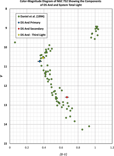
Figure 3. The color–magnitude diagram for the confirmed members of NGC 752 (filled circles) from Daniel et al. (1994) and the derived apparent magnitudes and color indices of the DS And system and its components (filled diamonds), free of third light, as noted in the text, although the error bars reflect possible systematic error. Note that the primary component is at the main-sequence turnoff and the secondary appears overluminous for a single star of its color index. The nearest star to it at the upper left on the "binary main sequence" is the overcontact binary QX And (=H235) and the bluest star on the plot is the blue straggler, H209.
Download figure:
Standard image High-resolution imageOur adopted systemic velocity, 8.13 ± 0.02 ± 0.50 km s−1, agrees with the mean cluster velocity, +9 km s−1, found by Rebeirot (1970), that of Friel et al. (1989), +8.5(30) km s−1, excluding a star with variable RV, and the mean velocity found by Pilachowski et al. (1988), 5.9(24) km s−1, from six stars that meet the proper motion criterion of Ebbighausen (1939) classes 1 and 2 (but without the exclusion of several stars for various reasons, leaving a mean of +4.9(7) km s−1). It is inconsistent with the adopted cluster velocity of Daniel et al. (1994), +5.5(6) km s−1, based on 33 stars but excluding stars differing by 3σ from the mean. On the other hand, it should be noted that the distribution of high-precision radial velocities found by Maderak et al. (2013) peaks at +5.4(1) km s−1 but the core histogram spans the range 2 to 8 km s−1, so it may be possible to set the RV criteria too narrowly. Moreover, our FIES RVs are highly precise and accurate but it has been suggested that if all RV results were reduced to the IAU or other uniformly accurate system, agreement might be closer. DS And's proper motion is also supportive of membership. Ebbighausen (1939) assigned it to class 2, with a reasonable chance of being a cluster member; the probability of membership was rated at >99% by Francic (1989), and at 99% by Platais (1991), whose catalog indicates the values μx = 7.9 and μy = −6.4 mas yr−1, where (x, y) are closely equatorial, with an estimated uncertainty of about 1.5 mas yr−1. The Gaia DR2 lists the proper motion components as μα = 10.72(8) and μδ = −11.78(8) mas yr−1. Thus, the preponderance of sky location, CMD locations, distance, extinction and metallicity, RV, and proper motion evidence is supportive of cluster membership.
6.2. The Evolutionary Status of DS Andromedae
The primary and secondary stars, free of third light, are placed on the CMDs in Figures 3 and 4. The primary is seen to be just at the turnoff point of the cluster and the secondary to be sitting roughly on the "binary main sequence," i.e., with brightness about twice that of a single star of its color index. Figure 4 displays the WEBDA V versus (V – RC) CMD, with three sets of Padova isochrones and binary sequences scaled to log age = 9.20 or 1.58 Gyr, (m–M)0 = 8.39, and for a metallicity of −0.08 (slightly different than the bulk of our models but within the range of the metallicities tested in the trials described in Section 3). The third-light-free V and (V – RC) of the system and components are superimposed as crosses. Sets of curves are shown for models with metals fractions Z = 0.004, 0.008, and 0.019. The lighter curves are the "binary sequences." A log age 9.20 model seems to provide a better fitting than the 9.15 or 9.25 models provided by this online source. If these models are appropriate for NGC 752, Z would need to lie closer to 0.008 than 0.019 to fit (if crudely) both the main-sequence and the giant branch, but a younger cluster implies a larger Z. The primary component is seen to be near or slightly below the main-sequence turnoff region, and on the Z = 0.008 isochrone curve. The secondary, just to the blue of this isochrone, does not seem to deviate very much from other later type main-sequence stars in the cluster, but neither does it appear to be on the same isochrone as the primary or at least not one with the same metals fraction. A similar result is found with Geneva isochrones, which are ∼0.02–0.04 mag bluer. Figure 5 places the components, labeled 1 and 2, on a log  versus log T plot amid isochrones for a range of ages. The isochrones are plotted from data in the online tables provided at http://stellar.dartmouth.edu/models/grid.html incorporating the empirical BVRCIC photometry of VandenBerg & Clem (2003) and, if we understand correctly, the VandenBerg et al. (2006) values of the He fraction Y = 0.2696, metals fraction Z = 0.016115, and α-element abundance α/Fe = 0.00. If these convective overshoot models with solar composition, metallicity, and helium fraction theoretical models are appropriate for the DS And system, the age of the primary is about 1.55(5) Gyr, significantly different from that found by Agüeros et al. (2018), 1.34(6) Gyr, but not significantly more than that found for NGC 752 by Twarog et al. (2015), 1.45(5) Gyr; not significantly less than that found for convective overshoot isochrone fitting to the cluster's main sequence by Daniel et al. (1994), 1.7(1) Gyr; and effectively the same as that found by Girardi et al. (2002), 1.55(10) Gyr. In this plot, the secondary appears to be noncoeval with the primary, a circumstance that appears to be confirmed in Figures 6 and 7, adapted from plots kindly provided by D. A. VandenBerg (2017, private communication). The evolutionary tracks plotted in Figures 6 and 7 are for overshoot models with Z = 0.013, and Z = 0.0188, respectively. The large dots on the tracks mark equivalent evolutionary phase (eep) points. The placements of the components among the tracks suggest that although both components are approximately in the expected regions for their masses, the secondary appears to be slightly older than the primary, as gauged by the evolutionary phase points. We note that the components appear to be closer to the appropriate track for their masses in Figure 6 than in Figure 7.

Figure 4. The V vs. V – RC color–magnitude diagram of NGC 752 from WEBDA (source given as Taylor et al. 2008) from which double-lined binaries have been excluded. Large crosses indicate the third-light-free components 1, 2, and 1+2 ("system") of the DS And system. The Padova model isochrone for log age = 9.20, scaled to (m – M)0 = 8.39, and a metallicity of −0.08, is also shown, for three metals fractions (0.004 in green (left), 0.008 in blue (middle), and 0.019 in red (right)); the less heavy curves mark the "binary sequence" for each. Unfilled circles signify members with a membership probability less than 0.50. See the text for further comments.
Download figure:
Standard image High-resolution image
Figure 5. The components of DS Andromedae superimposed on the solar composition isochrones of VandenBerg et al. (2006). In these models, Y = 0.2969 and Z = 0.0161. Note that the primary component (blue filled square) falls roughly on the 1.55 Gyr isochrone, whereas the secondary (red filled square) is too luminous for any of the isochrones. See the text for further details.
Download figure:
Standard image High-resolution image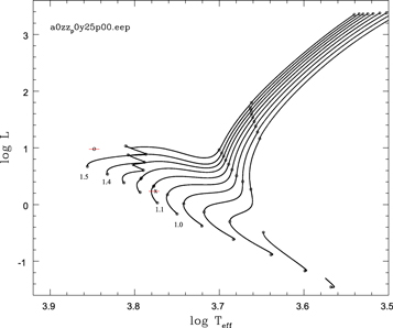
Figure 6. Overshoot model evolutionary tracks for solar composition stars of masses 0.5 through 1.5 MSun in steps of 0.1 MSun, kindly supplied by D. A. VandenBerg. In these models, the solar metals fraction, Z = 0.0133. Luminosity, L, is in solar units. The primary and secondary stars are respectively represented by ∘ and ×, the size of which approximates the formal uncertainties in the luminosities and temperatures; the red horizontal lines indicate uncertainties of ∼130 K. Although the 1.6 MSun track is not shown, the placements of the components are in rough accord with their masses, but not with respect to the equivalent evolutionary phase (eep) points indicated by open circles along the tracks. The components appear to differ slightly in age, but if the luminosity of star 2 were reduced by ∼0.22  , the difference would appear negligible.
Download figure:
Standard image High-resolution image
Figure 7. Overshoot model evolutionary tracks for solar composition stars of masses 0.5 through 1.7 MSun in steps of 0.1 MSun, kindly supplied by D. A. VandenBerg. In these models, the solar metals fraction Z = 0.0188. The primary and secondary stars are marked respectively by ∘ and ×, the sizes of which approximate the formal uncertainties in the average temperatures and luminosities; the red horizontal lines indicate an assumed systematic uncertainty of ∼±130 K in temperature. Assuming the models are applicable to DS And, the placements are roughly in accord with the masses; the apparent difference in eep becomes negligible if  is reduced by ∼0.22
  , as in Figure 6.
Download figure:
Standard image High-resolution imageA vertical shift with respect to the isochrones is explained if the secondary is overluminous compared to single star models (see Figure 5) perhaps because of its proximity to a hotter, larger, and much more luminous companion. A lower luminosity would bring it much closer to the evolutionary phase point of the primary star in Figures 6 and 7. Following a suggestion by G. Torres, the components are placed in an R versus M plane in Figure 8, with a selection of VandenBerg et al. (2006) isochrones for models with the same properties as in Figure 5. The radii are not listed in the tables but were computed from log g and mass values. The secondary appears to be too large for its mass, but the primary appears to be smaller than expected for its mass, if the models are appropriate. In Figure 9, the mass and radius of the primary and secondary stars are compared with the well-established masses and radii of the components of selected binary stars of similar spectral types (filled symbols), listed by Torres et al. (2010, Table 2). The Sun is also shown for reference. The secondary's mass and radius are similar to those of Alpha Cen A [G2V, M = 1.105(7) MSun, R = 1.224 RSun, in a wide binary with P = 79.91 yr]. This star is cooler (5824(26) versus 5971(33) K) and more metal-rich ([Fe/H] = 0.24(4)) than the DS And secondary. The primary's mass and radius are similar to those of FS Mon A (F2V, M = 1.632(10) MSun, R = 2.052(12) RSun, in a 1.91 day binary). This star is significantly cooler than the DS And primary [6715(100) versus 7056(21) K], but its metallicity is not given and was assumed to be 0.00. The temperature differences show that the stars are not exactly analogs and thus offer only weak support for the idea that the DS And components are anomalous, given systematic error estimates in T1,2 of ∼150 K, but neither can the idea be ruled out. The masses and radii calculated with the polynomial representation of log T, log g, and [Fe/H] terms (Torres 2010, Tables 1 and 3) are depicted by the unfilled and starred symbols. The differences between the determined and calculated values for the DS And components are in the range of those shown for the other stars (marked by red lines). The (lighter) regression line for the calculated points closely matches that of the stars themselves. Note that both DS And components fall close to the regression line for the plotted stars. We conclude that the primary may be somewhat radiatively anomalous compared with generic solar models and with stars of similar properties, but the secondary is certainly anomalous (already clear from its location on the CMD), but specific theoretical modeling needs to be done to check this conclusion. Another example of an oversized if cooler than expected star in a close binary of solar composition is EF Aqr B (M = 0.946(6) MSun, R = 0.956(12) RSun in a 2.85 day binary; Vos et al. 2012. It has a high rotational velocity (18(4) km s−1) due to synchronicity, but far less than DS And B's 63 km s−1. Strikingly (see below), EF Aqr is an X-ray source, and strong magnetic fields have been invoked to suppress its envelope convection. There are many other cases (see Feiden & Chaboyer 2012, 2014) with similar anomalies. Fekel's (1997) Table 1 shows that early FV and early GV stars' v sin i measurements typically fall within ranges of 10–20 and 1–10 km s−1, respectively. Thus, rotational speed-up may be key to DS And's anomalies. There are at least two other anomalous objects with very similar proper motions and high probability of membership in NGC 752 (Platais 1991): QX And (H235), the only overcontact system in the cluster, and the blue straggler H209, so prominently visible on the extreme left in Figures 3 and 4. Both are among eight NGC 752 objects detected in X-rays (Belloni & Verbunt 1996), with DS And, lying just outside the inner region of the detector, as a possible detection (Van den Berg & Verbunt 2001 describe this as a probable detection). The X-ray luminosities of QX And, H209, and DS And are given, respectively, as 7.4 × 1029, 6.7 × 1029, and 2.9 × 1030 erg s−1. Like DS And, QX And is a close binary with a variable light curve and with at least one component that is likely magnetically active, but the circumstance for H209 is different. It is a very wide spectroscopic binary with a period of 1574 days (Van den Berg & Verbunt 2001, citing a private communication from D. Latham), and no very close companion has been detected spectroscopically by Van den Berg & Verbunt (2001). Those authors conclude that the cause of the X-ray emission and blue straggler nature of H209 is unknown. Twarog et al. (2015) noted that its age with respect to the Victoria–Regina isochrones is less than 0.1 Gyr. It is possible that H209 is a merger product of a former close binary, and so "reborn"; in any case, it is an anomalous object. Considering that such evolved binaries are not to be expected in an "intermediate-age" cluster unless they have lost angular momentum to wider components, the three anomalous objects would suggest that a dedicated search for wider components in these binary systems is in order.
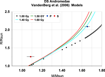
Figure 8. The primary (blue filled circle) and secondary (red filled square) components of DS And superimposed on the isochrones of the solar composition models of VandenBerg et al. (2006) in the radius vs. mass plane, where the radius is computed from the tabulated log g entry. In these models, Y = 0.2696 and Z = 0.0161. The error bars indicate conservative systematic error estimates for M1,2; those for the R1,2 are symbol-high. The secondary appears to be anomalously large for its mass whereas the primary is too small relative to the 1.5 and 1.6 Gyr isochrones, if the models are appropriate for this system. The secondary's bloated nature could be a possible result of its proximity to a larger and hotter companion and/or its spin-up due to synchronicity.
Download figure:
Standard image High-resolution image
Figure 9. The radii and masses of the DS And primary (P: blue filled circle) and secondary (S: red filled square) components of DS And are plotted along with those of selected stars in Torres (2010, Table 1) and EF Aqr (green-filled diamonds, "R" in the legend), and representations of the mass and radius by their polynomial functions of log Teff, log g, and [Fe/H] (star symbol), joined to the corresponding filled symbols by red lines. The linear regression line for the filled symbols is darker than that for the calculated radii. Note the similarity of the M and R of the DS And secondary to Alpha Cen A (G2V), and the primary to FS Mon A (F2V). See text for further details.
Download figure:
Standard image High-resolution image
7. Summary and Conclusion
We have carried out extensive modeling of the ESB2 binary DS Andromedae, making use of the direct distance estimation algorithm in the 2013 version of the Wilson–Devinney program to determine the distance as a system parameter. We used the well-calibrated BVRCIC photometry previously discussed in Schiller & Milone (1988), 94 U observations not previously reported, and new RV data of Mellergaard Amby (2011). A great number of runs of ∼70 individual models were carried out, and extensive trials and tests were investigated to test the robustness of the parameter means. Although the bulk of the modeling was performed on detached models, series of semidetached models were also run. We found mode 4 semidetached models (in which the primary star fills its Roche lobe) to be non-convergent and mode 5 SD models (in which the secondary star does so) to yield higher mean residuals than the best detached models. The secondary star's anomalies remain unexplained because its luminosity in the mode 5 SD models is greater than in detached system models. The effects of varying the interstellar extinction, the stellar metallicity, and the passband calibration constants; of separating the RADS and non-RADS bands; of weighting of RADS data relative to non-RADS data; of the introduction of star spots; of the applications of detailed reflection and nonsynchronous rotation; of adjusting third light, and of adjusting the period derivative (P-dot) parameter were all explored. Finally, trials with previously excluded U data provided a check on the robustness of the solutions and parameter values. The most extensive modeling was carried out on detached system models, and after all the trials were concluded, this type of model was confirmed as yielding the lowest mean residuals. Weighted means of parameters were obtained from multiple runs of detached models that do not differ radically among themselves but are equally viable. The adopted Model 40 run means are confirmed by group means and the grand means. Assuming that the system's significant third light is stellar in origin, we determined the third-light-free magnitudes and color indices. The stellar models, although not strictly specific to our assumed cluster parameters, yield a similar age if the metals fraction Z is between ∼0.008 and 0.019. The luminosities and temperatures of the primary and secondary components of the DS And system superimposed on the model tracks of VandenBerg et al. (2006) for stars of solar composition reveal that the primary is evolved from the zero-age main sequence and lies near the 1.55 Gyr isochrone whereas the secondary is overluminous for its temperature and cannot fit any of the isochrones. Compared with overshoot models, the primary again appears to have an age of 1.5–1.6 Gyr; the secondary appears not to be coeval, but this may be explained by its being overluminous. In an R versus M isochrone plot, the secondary star appears to be too large for its mass by about 25%, and the primary too small by ∼10%. In short, we conclude that DS Andromedae is a detached system at a distance of 477 ± 4 ± 13 pc, and a likely, if not certain, member of NGC 752.
The help of R. E. Wilson with the WD 2013 program and earlier versions, and for unstinting advice and suggestions (if not always followed!) at several stages of this work, and formatting of Table 15 that is sampled in the Appendix, is acknowledged with gratitude. D. A. VandenBerg provided helpful advice and was kind enough to provide the evolutionary tracks shown in Figures 6 and 7. I. Platais provided his proper motion catalog. R. H. Nelson provided copies of his spreadsheets on DS And times of minimum. G. Torres was kind enough to comment on an earlier draft in fine detail, ran an independent analysis of the radial velocity data, and provided many helpful suggestions; other comments were provided by Peter Eggleton and Bruce Twarog. Doug Phillips, Senior Computational Science Consultant at the University of Calgary's Research Computing Services, helped with the migration of WD to different platforms. We acknowledge the facilities used by and the allocation of observing time to S.J.S. at the McDonald, Table Mountain, and Dominion Astrophysical Observatories. The current RVs are based on observations made with the Nordic Optical Telescope, operated by the Nordic Optical Telescope Scientific Association at the Observatorio del Roque de los Muchachos, La Palma, Spain, of the Instituto de Astrofisica de Canarias. This work has made use of BaSTI web tools, data from WEBDA, and data from the European Space Agency (ESA) mission Gaia (http://www.cosmos.esa.int/gaia), processed by the Gaia Data Processing and Analysis Consortium (DPAC, http://www.cosmos.esa.int/web/gaia/dpac/consortium). Funding for DPAC has been provided by national institutions, in particular those participating in the Gaia Multilateral Agreement. Data acquisition and research were supported by grants to E.F.M. from NSERC of Canada and by the Research Grants Committee and the Department of Physics & Astronomy of the University of Calgary. AAS Data and software editors Greg Schwarz and August Muench provided helpful suggestions as well as guidance in the access and use of the repository. Finally, an anonymous referee provided insightful criticisms and useful comments. We are appreciative of all this assistance.
Appendix:
The complete set of IC, RC, V, B, and U data are listed in Table 15 and is available in the Zenodo repository package 10.5281/zenodo.2553042. A short sample appears below.
Table 15. DS Andromedae Photometric Data
| HJD (Ic) | Ic | wt. | HJD (Rc) | Rc | wt. | HJD (V) | V | wt. | HJD (B) | B | wt. | HJD (U) | U | wt. |
|---|---|---|---|---|---|---|---|---|---|---|---|---|---|---|
| 2445243.7962 | 9.988 | 0.239 | 2445243.8226 | 10.227 | 0.157 | 2445243.8058 | 10.442 | 0.093 | 2445243.8094 | 10.822 | 0.088 | 2445600.8553 | 11.368 | 1.000 |
| 2445243.8200 | 9.981 | 0.239 | 2445243.8233 | 10.217 | 0.157 | 2445243.8065 | 10.468 | 0.093 | 2445243.8101 | 10.840 | 0.088 | 2445600.8560 | 11.347 | 1.000 |
| 2445243.8208 | 9.985 | 0.239 | 2445243.8240 | 10.249 | 0.157 | 2445243.8260 | 10.463 | 0.093 | 2445243.8124 | 10.832 | 0.088 | 2445600.8567 | 11.366 | 1.000 |
| 2445243.8338 | 9.955 | 0.239 | 2445243.8364 | 10.201 | 0.157 | 2445243.8267 | 10.455 | 0.093 | 2445243.8131 | 10.812 | 0.088 | 2445600.8577 | 11.359 | 1.000 |
| 2445243.8345 | 9.967 | 0.239 | 2445243.8371 | 10.214 | 0.157 | 2445243.8388 | 10.426 | 0.093 | 2445243.8284 | 10.832 | 0.088 | 2445600.8583 | 11.360 | 1.000 |
| 2445243.8464 | 9.935 | 0.239 | 2445243.8489 | 10.218 | 0.157 | 2445243.8395 | 10.456 | 0.093 | 2445243.8291 | 10.814 | 0.088 | 2445600.8590 | 11.369 | 1.000 |
| 2445243.8472 | 9.937 | 0.239 | 2445243.8497 | 10.211 | 0.157 | 2445243.8513 | 10.443 | 0.093 | 2445243.8415 | 10.840 | 0.088 | 2445600.8598 | 11.344 | 1.000 |
| 2445243.8722 | 9.952 | 0.239 | 2445243.8742 | 10.178 | 0.157 | 2445243.8519 | 10.436 | 0.093 | 2445243.8423 | 10.845 | 0.088 | 2445600.8626 | 11.358 | 1.000 |
| 2445243.8729 | 9.966 | 0.239 | 2445243.8749 | 10.228 | 0.157 | 2445243.8766 | 10.403 | 0.093 | 2445243.8537 | 10.830 | 0.088 | 2445600.8634 | 11.361 | 1.000 |
| 2445243.8865 | 9.957 | 0.239 | 2445243.8893 | 10.234 | 0.157 | 2445243.8773 | 10.452 | 0.093 | 2445243.8544 | 10.782 | 0.088 | 2445600.8641 | 11.364 | 1.000 |
| 2445243.8872 | 9.943 | 0.239 | 2445243.8900 | 10.228 | 0.157 | 2445243.8920 | 10.417 | 0.093 | 2445243.8790 | 10.840 | 0.088 | 2445600.8648 | 11.343 | 1.000 |
| 2445243.9060 | 9.980 | 0.239 | 2445243.9083 | 10.189 | 0.157 | 2445243.8927 | 10.465 | 0.093 | 2445243.8798 | 10.802 | 0.088 | 2445600.8656 | 11.350 | 1.000 |
| 2445243.9067 | 9.954 | 0.239 | 2445243.9090 | 10.212 | 0.157 | 2445243.9105 | 10.411 | 0.093 | 2445243.8943 | 10.834 | 0.088 | 2445600.8686 | 11.346 | 1.000 |
| 2445243.9261 | 9.971 | 0.239 | 2445243.9282 | 10.226 | 0.157 | 2445243.9112 | 10.445 | 0.093 | 2445243.8950 | 10.796 | 0.088 | 2445600.8693 | 11.352 | 1.000 |
| 2445243.9268 | 9.940 | 0.239 | 2445243.9289 | 10.220 | 0.157 | 2445243.9309 | 10.428 | 0.093 | 2445243.9127 | 10.830 | 0.088 | 2445600.8700 | 11.333 | 1.000 |
| 2445243.9377 | 9.972 | 0.239 | 2445243.9400 | 10.220 | 0.157 | 2445243.9316 | 10.440 | 0.093 | 2445243.9134 | 10.830 | 0.088 | 2445600.8706 | 11.347 | 1.000 |
| 2445243.9384 | 9.957 | 0.239 | 2445243.9408 | 10.216 | 0.157 | 2445243.9424 | 10.438 | 0.093 | 2445243.9332 | 10.818 | 0.088 | 2445600.8714 | 11.340 | 1.000 |
| 2445243.9572 | 9.998 | 0.239 | 2445243.9592 | 10.222 | 0.157 | 2445243.9431 | 10.455 | 0.093 | 2445243.9338 | 10.827 | 0.088 | 2445600.8741 | 11.342 | 1.000 |
| 2445243.9578 | 9.952 | 0.239 | 2445243.9599 | 10.207 | 0.157 | 2445243.9615 | 10.445 | 0.093 | 2445243.9448 | 10.859 | 0.088 | 2445600.8748 | 11.324 | 1.000 |
| 2445243.9689 | 9.947 | 0.239 | 2445243.9705 | 10.214 | 0.157 | 2445243.9622 | 10.452 | 0.093 | 2445243.9455 | 10.842 | 0.088 | 2445600.8755 | 11.354 | 1.000 |
| 2445243.9796 | 9.978 | 0.239 | 2445243.9712 | 10.229 | 0.157 | 2445243.9727 | 10.470 | 0.093 | 2445243.9636 | 10.856 | 0.088 | 2445600.8762 | 11.319 | 1.000 |
| 2445243.9803 | 9.961 | 0.239 | 2445244.0062 | 10.251 | 0.157 | 2445243.9734 | 10.479 | 0.093 | 2445243.9642 | 10.844 | 0.088 | 2445600.8789 | 11.336 | 1.000 |
| 2445244.0039 | 9.990 | 0.239 | 2445244.0069 | 10.268 | 0.157 | 2445243.9840 | 10.454 | 0.093 | 2445243.9750 | 10.880 | 0.088 | 2445600.8797 | 11.323 | 1.000 |
| 2445244.0046 | 9.969 | 0.239 | 2445244.0254 | 10.266 | 0.157 | 2445243.9847 | 10.440 | 0.093 | 2445243.9757 | 10.830 | 0.088 | 2445600.8805 | 11.340 | 1.000 |
Download table as: ASCIITypeset image
Footnotes
- *
Publications of the RAO No. 77.