


Abstract
Various simplified models have been investigated as a way to understand the complex dynamical environment near irregular asteroids. A dipole segment model is explored in this paper, one that is composed of a massive straight segment and two point masses at the extremities of the segment. Given an explicitly simple form of the potential function that is associated with the dipole segment model, five topological cases are identified with different sets of system parameters. Locations, stabilities, and variation trends of the system equilibrium points are investigated in a parametric way. The exterior potential distribution of nearly axisymmetrical elongated asteroids is approximated by minimizing the acceleration error in a test zone. The acceleration error minimization process determines the parameters of the dipole segment. The near-Earth asteroid (8567) 1996 HW1 is chosen as an example to evaluate the effectiveness of the approximation method for the exterior potential distribution. The advantages of the dipole segment model over the classical dipole and the traditional segment are also discussed. Percent error of acceleration and the degree of approximation are illustrated by using the dipole segment model to approximate four more asteroids. The high efficiency of the simplified model over the polyhedron is clearly demonstrated by comparing the CPU time.
Export citation and abstract BibTeX RIS
1. Introduction
Small celestial bodies, which include asteroids, comets, and planetary moons, are a central topic in current deep-space exploration because of their significance for the evolution of our solar system, among other reasons. Because of a small body, irregular shape, and state of rotation, the description of their corresponding gravitational field is one of the most challenging problems in asteroid exploration missions and astrophysical studies. Representations of an asteroid's irregular gravitational field include the polyhedral model (Werner 1994; Werner & Scheeres 1997), the gravity potential series expansion (Kaula 2000), the mascons model (Geissler et al. 1996), and other simplified models (Bartczak et al. 2006). The polyhedral method is one of the most widely used methods with relatively high precision. Another high-precision method is the mascons model (Geissler et al. 1996), which employs a group of point masses to render the mass distribution within the asteroid.
Both the polyhedron and mascons are usually adopted to evaluate the gravitational field of a specific asteroid given its geometry information. These two methods require long computation time, which increases as more facets or point masses are introduced into the representation. However, when a spacecraft or a test particle is sufficiently far away from the asteroid surface, the efficiency of these two methods is relatively low for orbit propagation. The series expansion method with Legendre polynomials is numerically efficient for spheroid-like planets (such as major planets, 1 Ceres, or 4 Vesta) but seldom converges in close proximity to the asteroid surface (Riaguas et al. 1999; Bartczak et al. 2006). As an alternative simplified model, a triaxial homogeneous ellipsoid is a good approximation for the gravity potential function of Eros-like asteroids (Bartczak & Breiter 2003). However, as a drawback of adopting elliptical integrals, analytical results are more difficult to obtain (Bartczak et al. 2006).
By extracting the main features of irregular bodies, simplified models help in understanding the fundamental dynamical behaviors of a particle orbiting within an asteroid system. To efficiently approximate the gravity potential function of irregular asteroids, a few simplified models have been proposed with analytical potential forms. The initial material segment model proposed by Duboshin (1959) was mainly extended by works from Bartczak & Breiter (2003), and Breiter et al. (2005), among others (Najid et al. 2011; Romanov & Doedel 2014). In particular, Bartczak et al. introduced an asymptotic adjustment method by comparing the Legendre series of segment-like models with classical spherical harmonics. Based on the asymptotic method, it was also demonstrated that the material segment model provides a better approximation for a spheroidal mass distribution than a pair of material points (Bartczak et al. 2006). Note that the two material points used by Bartczak et al. (2006) are equal in mass, thus rendering a special case of the dipole model (Chermnykh 1987).
Simplified models may be a valid, computationally less demanding alternative to a sophisticated polyhedron or mascons model for predicting particle orbital motion near asteroids (Bartczak & Breiter 2003). With an analytical form for the asteroid potential function, Elipe & Lara (2003) analyzed the chaotic motion around Eros by using a rotating segment. However, the approximation from Elipe & Lara (2003) displays large errors in accelerations, which is reported in the Appendix of this study. Unfortunately, large acceleration errors cannot be accepted even for qualitative analyses.
The approximation quality, as measured by the acceleration error, may be improved in two ways: one is to optimize the parameters of the segment model to reduce acceleration error; the other is to incrementally increase the complexity of the material segment model. That leads us to the question: What approximation accuracy can be obtained by using an optimized material segment model to describe real asteroids? Moreover, is there any other efficient simplified model that is better than the homogeneous material segment? Such questions serve as motivation for the following investigation.
A material segment may approximate the exterior potential distribution of elongated bodies as an equivalent cylinder. However, most elongated minor celestial bodies have a larger head part, similar to the asteroid (8567) 1996 HW1 (seen in Figure 5). To preliminarily evaluate the mass ratio between the two head parts, the dipole model (Yang et al. 2015; Zeng et al. 2016, 2017) can be applied, particularly when the two parts have different density, such as in the asteroid 25143 Itokawa (Lowry et al. 2014).
Chermnykh (1987) started the investigation of the Lyapunov stability of the triangular points of the rotating dipole system. Goździewski & Maciejewski (1998, 1999) extended Chermnykh's work by varying the system parameters and further considered a mutual potential generated by a dipole and a point mass. It seems to the authors (Zeng & Alfriend 2017) that Prieto-Llanos & Gómez-Tierno (1994) independently derived the dipole model by generalizing the classical three-body problem. One application is also given for the Mars–Phobos system to stabilize a spacecraft near the collinear L1 point (Prieto-Llanos & Gómez-Tierno 1994).
For the Mars–Phobos system or binary asteroids, the dipole model may be a good approximation, representing the two system primaries as point masses. However, for an elongated asteroid, the dipole model poorly describes the neck region. When approximating an irregular body, the system mass and the rotating period of the simplified model are usually set to be the same as the irregular body (Bartczak & Breiter 2003; Elipe & Lara 2003; Bartczak et al. 2006). Such a choice indicates that only the segment length is a free parameter. As for the dipole model, two independent system parameters exist, including its characteristic length and the mass ratio between the two point masses.
In order to improve the degree of the gravity potential function approximation for elongated asteroids (especially the dumbbell-shaped or contact-binary types), a dipole segment model is proposed in this study. Topological cases of the new model are introduced in Section 2. Dynamical equations of a test particle are derived with a detailed discussion on the force ratio. In Section 3, system equilibria are investigated in a parametric way, exploring their bifurcations, stability, and variational trends. In Section 4, application of the dipole segment to the asteroid 1996 HW1 is demonstrated. A practical method is proposed to obtain optimized parameters of the dipole segment, by minimizing the acceleration error in the equatorial plane over the polyhedral model. A comparison among the dipole segment, the classical dipole, and the traditional segment is made in the potential approximation of HW1. Four more potential approximations are presented for 951 Gaspra, 2063 Bacchus, Itokawa, and 103P/Hartley-2. Additionally, the efficiency of the dipole segment model over the polyhedron is illustrated by comparing the CPU time. In Section 6 some final remarks conclude the paper.
2. Dynamical Equations of the Dipole Segment
The dipole segment comprises a finite, homogeneous straight segment and two point masses fixed at its ends. Denote m1 and m2 the two point masses, such that M1 = m1 + m2. The segment mass is labeled M2, and the total system mass is M = M1 + M2. Let's introduce two mass ratios

which take values within the ranges μ1 ∈ [0, 0.5] and μ2 ∈ [0, 1], respectively. Five topological cases are shown in Figure 1 (left) for this model. When the mass ratio μ2 is exactly equal to zero, the system degenerates to trivial cases: either a single point mass or a classical dipole model. If the mass ratio μ2 is unitary, the traditional segment model is obtained. Since these three limiting cases are discussed in previous publications, only the other two cases for  are the focus of the current study.

Figure 1. Five topological cases of the dipole segment and its body-fixed frame.
Download figure:
Standard image High-resolution imageIt is convenient to define a body-fixed frame oxyz where the origin o is at the system center of mass. Axis ox is aligned with the segment pointing from m1 to m2. Axis oz is along the direction of the spin velocity  , while axis oy completes the right-hand frame, as displayed in Figure 1 (right). Supposing the segment has constant density ρ, the segment length can be obtained as l = M2/ρ = l1 + l2. Unlike the massless rod of the classical dipole model, it should be possible to analyze cohesive forces of the inner structure of asteroids by using the dipole segment with appropriate assumptions.
2.1. Potential of a Dipole Segment
The gravitational potential of the dipole segment at a certain position ![${\boldsymbol{r}}={[x,y,z]}^{{\rm{T}}}$](https://content.cld.iop.org/journals/1538-3881/155/2/85/revision1/ajaaa483ieqn3.gif) can be expressed in a simple form as
can be expressed in a simple form as

where G is the gravitational constant, and  ) is the distance to the corresponding primary. As shown in Figure 1, the two position vectors are written as

The line integral in the third term on the right represents the gravitational attraction of the segment, which is given with

Substituting the above equation and mass ratios into Equation (2) yields
The potential function depends on the total system mass, segment length, position vectors, and mass ratios. Particularly, the potential function is symmetrical with plane oxy and plane oxz. Therefore, application of the dipole segment model is limited to approximating an actual asteroid without considering nonsymmetrical mass distributions along the oy and oz directions.
2.2. Equations of Motion
Assume the dipole segment is rotating with a constant angular velocity. The vector equations of motion of a test particle that is attracted by the dipole segment are

in the body-fixed frame oxyz shown in Figure 1. As the centrifugal term is conservative, the above equation is reorganized by introducing an effective potential V, such that

For convenience, the equations of motion are nondimensionalized during numerical computations. The length unit LU is taken to be l and the mass unit MU is M. The time unit TU is equal to  , resulting in a 2π TU segment rotation period. Accordingly, the nondimensional effective potential is
where the scalar parameter κ is referred to as the "force ratio", representing the ratio between the gravitational and centrifugal accelerations with

Note that the variables x, y, r1, and r2 in Equation (8) are already in dimensionless units. The nondimensional position vectors are written by introducing a new auxiliary parameter ν = l2/l, yielding
Using the center of mass equation
one can obtain the following relationship:

Here, ν is always within the range [0.5, 1). For example, if both μ1 and μ2 are 0.5, the value of ν is 0.5, which is consistent with the physical intuition that the mass center should be at the midpoint of the segment. The case of ν = 1 is excluded, corresponding to the case of a single point mass with μ1 = μ2 = 0.
Notice that Equation (7) is expressed in the body-fixed frame and yields an autonomous system in a six-dimensional phase space [x, y, z,  ,
,  , ż]T. Therefore, an energy integral can be obtained, one that corresponds to the Jacobi constant

The Jacobi constant determines the region of allowable motion for a test particle. Substituting Equations (8), (10), and (12) into Equation (7) yields the equation of motion for each position component,

where the partial derivatives of the effective potential function in the right-hand terms of the above equations are

2.3. Discussion on the Force Ratio
In the potential approximation for irregular asteroids, the angular velocity  of the simple model is typically the same as the actual system as well as the total system mass (Bartczak & Breiter 2003; Elipe & Lara 2003; Bartczak et al. 2006). Then, the value for three independent parameters of the dipole segment, that is, [κ, μ1, μ2]T, remains to be assigned. From Equation (9) there is a one-to-one correspondence between the force ratio κ and the characteristic length l. Accordingly, the three free parameters can also be chosen as [l, μ1, μ2]T.
The value for the force ratio κ is a key parameter in analyzing the irregular gravitational field of an asteroid. In the following discussion, a method to determine the force ratio is explored. Assume the constant-density polyhedral model of the asteroid is a sufficiently accurate representation of the gravity potential. Results from the polyhedron serve as reference values. When a test particle is gravitationally attracted by an irregular asteroid within the polyhedral model, the potential in Equation (2) is changed to an integral over the volume as

where the subscript P denotes the polyhedron. The parameter  is a constant density and can be extracted from the integral,
  is the total system mass, and r is the same distance as in Equation (2). The integral of the volume
  (Werner & Scheeres 1997) is difficult to handle. By substituting Equation (18) into Equation (6), one can obtain the particle equations of motion within the polyhedral model:

The length and time units

are employed to nondimensionalize Equation (19). The length unit  corresponds to the radius of an equivalent spheroid with the same volume as the asteroid. The dimensionless form for the equations of motion in Equation (19) is

where  is the dimensionless position vector
  , and
, and ![${\boldsymbol{\Omega }}={[0,0,1]}^{{\rm{T}}}$](https://content.cld.iop.org/journals/1538-3881/155/2/85/revision1/ajaaa483ieqn15.gif) denotes the angular velocity. The dimensionless parameter
denotes the angular velocity. The dimensionless parameter  , similar to the force ratio in Equation (9), is

For an actual asteroid, its rotating period can be determined with observation data. The bulk density can be obtained from the estimated volume and system mass of the asteroid based on the albedo or variations of the light curve (Magri et al. 2011). When we use the dipole segment to approximate an elongated asteroid, the system parameters are set to be M =  and l = ε
  , where ε is a positive coefficient. With these conditions, one can obtain

In the above equation, a relationship in terms of the force ratio has been established between the simplified and polyhedral models. It also reveals the relationship between the characteristic length of the simplified model and the equivalent spheroid of an asteroid. It can be treated as an improvement of previous efforts made by Elipe & Lara (2003), Hirabayashi et al. (2010), and Zeng et al. (2015).
3. Equilibrium Points and Their Stability
Equilibrium points are important to understand the topological features of a dynamical system. They are stationary points of the effective potential. Unlike ideally spherical planets, irregular asteroids usually hold a finite number of isolated equilibria, as discussed by Wang et al. (2014). Most asteroids, including 243 Ida, Eros, Gaspra, 1996 HW1, and a spheroid-like Vesta, have four exterior equilibrium points. According to previous results, there are five equilibrium points for the classical dipole model, similar to the restricted three-body problem (CRTBP). On the contrary, the inner equilibrium point L1 does not exist for the straight segment. In this section, the equilibria of the dipole segment are investigated by varying the parameters of the model.
3.1. Equilibrium Points of the Dipole Segment
One of the simplest cases for the dipole segment model is a degenerated, single point mass case, as displayed in Figure 1, which corresponds to μ1 = μ2 = 0. There is an infinite number of equilibrium points in the stationary orbit with radius r = ![$\sqrt[3]{{GM}/{\omega }^{2}}$](https://content.cld.iop.org/journals/1538-3881/155/2/85/revision1/ajaaa483ieqn19.gif) . Furthermore, if
. Furthermore, if  and μ2 is still zero, the dipole segment is transformed into the classical dipole model. Moving from a single point to two rotating point masses with a fixed distance, the number of system equilibria becomes finite. Five or three points can be appear, depending on the parameters of κ and μ1. The stability for those equilibria can be found in Prieto-Llanos & Gómez-Tierno (1994) and Hirabayashi et al. (2010). If μ2 = 1, there are four equilibria for the traditional segment model (Romanov & Doedel 2014). A detailed discussion on the linear and nonlinear stability of the four equilibrium points refers to Riaguas et al. Bifurcations of equilibria for the above three conventional cases of the dipole segment model are briefly summarized as a reference. The number and locations of equilibria for the general dipole segment model will be studied in detail as follows.
Due to the symmetrical property with respect to the plane oxy, all of the equilibria of the dipole segment are located in the equatorial plane. The collinear equilibria can be obtained with the following conditions:

whereas the triangular (or noncollinear) equilibria must fulfill

From the above two equations, Equation (17) is always zero with z = 0. When y = 0, the collinear equilibrium points can be achieved by solving Equation (15) as a seventh-order polynomial function of x:

where the subscript CE denotes the collinear equilibrium points. The explicit expressions of the coefficients ci are relatively lengthy. Therefore, only the first three coefficients are demonstrated, yielding

If there is an inner equilibrium point on the segment similar to the L1 point of CRTBP, the sum of the two distances r1 and r2 between the point and the two primaries is exactly unity in dimensionless units. It results in a zero value of the term 1 − (r1 + r2)2 in the denominator of Equations (15)–(17), corresponding to a singular case. Hence, no inner equilibrium point exists for the dipole segment model. There are only two collinear equilibria for the general dipole segment with  . The locations of these two collinear points lie within the respective ranges

The triangular equilibria of Equation (25) can be deduced from the set of equations

It is difficult to analytically solve the above equations for the general dipole segment model. Nevertheless, its solution can be examined from particular cases. For instance, if  and μ2 = 0, corresponding to the classical dipole model, Equation (28) can be simplified by considering Equation (12) as r1 = r2 = κ3. By combining Equation (10), the solution for the above equations can be given as

which is the same as the result reported by Prieto-Llanos & Gómez-Tierno (1994).
Moreover, if μ2 = 1 (resulting in μ1 = 0 and ν = 1/2), corresponding to the traditional segment, one can easily obtain r1 = r2 from Equation (28). For the segment, the coordinates of triangular equilibria are in the form [0, y, 0]T. By substituting r1 = r2 into any one of the Equation (28), the solution is that the y coordinate satisfies the following equation:
which is consistent with the result of Romanov & Doedel (2014). Note that the dimensionless units between Romanov & Doedel (2014) and our study are different. The length of the segment is two in Romanov & Doedel (2014) and unity for us.
The triangular equilibria for the general dipole segment can be obtained by numerically solving Equation (28) via a Newton method. As an example, consider the symmetrical case with  and μ1 = μ2 = 0.5. This choice of parameters indicates that there is no cohesive force in the model and the dipole segment is symmetrical with all three coordinate planes. Figure 2(a) illustrates the equilibrium points and section view of zero-velocity surfaces that are obtained numerically. There are four equilibria in total: E1 [−1.1499, 0, 0]T, E2 [+1.1499, 0, 0]T, E3 [0, −0.9199, 0]T, and E4 [0, +0.9199, 0]T. Zero-velocity surfaces indicate the motion boundaries with C = V in Equation (13). As the variables are in dimensionless units, the length of the dipole segment in Figure 2 is exactly unitary. A comparison of locations of equilibria with the dipole (μ2 = 0.0) and segment (μ2 = 1.0) are given in Table 1. As Ei (i = 1, 3) are symmetrical with Ei+1, only E1 and E3 are listed.

Figure 2. Equilibrium points of the dipole segment and section view of zero-velocity surfaces.
Download figure:
Standard image High-resolution imageTable 1. Comparison of Equilibrium Points among Different Simplified Models
| κ = 1, μ1 = 0.5 | Dipole segment μ2 = 0.5 | Classical dipole μ2 = 0.0 | Traditional segment μ2 = 1.0 |
|---|---|---|---|
| E1 | [−1.1499, 0, 0]T | [−1.1984, 0, 0]T | [−1.0832, 0, 0]T |
| E3 | [0, −0.9199, 0]T | [0, −0.8660, 0]T | [0, −0.9608, 0]T |
Download table as: ASCIITypeset image
Table 2 illustrates the displacement direction of the equilibrium points with respect to the central body as the three parameters [κ, μ1, μ2]T are varied for the case  . The symbol
  denotes that the corresponding parameter is increasing, while
  is used for parameters that are fixed. Directional arrows indicate the moving direction of coordinates of the equilibria along with the variation of parameters. For instance, for fixed values of κ and μ1, the collinear equilibria E1 and E2 move inward by increasing μ2. The triangular equilibria in contrast move outward with the increase of μ2.
Table 2.
Variation Trends of Coordinates for the Equilibria with the System Parameters for 
| x(E1) | x(E2) | x(E3) | y(E3) | |
|---|---|---|---|---|

|

|

|

|

|

|

|

|

|

|

|

|

|

|

|
Download table as: ASCIITypeset image
It can also be confirmed that, for fixed mass ratios, all of the four equilibria move away from the central body with the increase of the force ratio κ. By increasing μ1 with fixed values of κ and μ2, the system center of mass moves toward the midpoint of the segment. Meanwhile, the x coordinates of all equilibria move along the -x direction, and the triangular points move outward along the axis oy. Figure 2(b) portrays the distribution of the equilibrium points for the special case with μ1 = 0. The geometric shape of the near-realm, zero-velocity surface is similar to that of the asteroid Gaspra, which is very different from the symmetrical case of Figure 2(a).
The two triangular points of the classical dipole model (μ2 = 0) vanish when the value of κ is not greater than 0.125 (Prieto-Llanos & Gómez-Tierno 1994). However, such a property is not found for the dipole segment with  through our numerical simulations. Figure 3 gives an example by illustrating the case of μ2 = 0.8 for each constant value of μ1. The lowest boundary value of κ is taken to be
  (far less than 0.125) to avoid misleading by numerical precision. The upper boundary value of κ is 0.5 with a step of
  to be gradually decreased to its end of
  in a number of total 250. Seven discretized values of μ1 are selected with [0.01, 0.05, 0.1, 0.2, 0.3, 0.4, 0.5]T. Each curve shows the variational trend of the triangular equilibrium point E4 along with the decreasing of κ. Since the two triangular equilibrium points are symmetrical with respect to the axis ox, the other point E3 is not given. The arrow shows the variational direction of the equilibrium point where the circle marker "o" denotes E4.

Figure 3. Variation of the E4 location by decreasing κ from 0.5 to  for the case of μ2 = 0.8 with different values of μ1.
Download figure:
Standard image High-resolution imageFrom Figure 3, the y coordinate of the point E4 decreases along with the decrease of κ. Nevertheless, for all sample values of μ1, the y coordinate of E4 is not zero even with  . Thus, the introduction of the parameter
  makes the bifurcation property of the dipole segment different from the classical dipole model. In other words, when
  , the triangular equilibrium points do not vanish even for a very small value of κ, which is much less than the critical value of 0.125 for the rotating dipole model. It indicates that the existence of the segment between the two point masses prevents the vanishing of the triangular points.
Figure 4 shows another variational trend of E4 by decreasing the value of μ2 from 1.0 to 0.0 in a step of 0.1. Sample values of μ1 are the same as given in Figure 3. The force ratio κ is taken to be 0.1 in a value less than 0.125, which is used to evaluate the bifurcation. In fact, there are topological transitions for the central simplified model corresponding to the above choice of μ2, that is, from traditional segment (μ2 = 1.0) to the general dipole segment and finally to the classical dipole (μ2 = 0.0). Therefore, all seven sample curves start from the same initial position of E4 right above the origin on the oy axis. With the decrease of μ1, the x coordinate of E4 increases, which is consistent with Table 2 but not the focus here. Seven circle markers "o" representing the equilibrium point are finally located on the axis ox when μ2 = 0.0. Such a bifurcation caused by the topological transition of the model indicates that the triangular equilibrium point E4 (as well as E3) vanishes and a new collinear equilibrium point between the two point masses emerges. It also tells us that the characteristic of the equilibrium point changes from the triangular point to the collinear point. By considering all equilibrium points for the dipole segment, this bifurcation leads to the variation of the number of equilibria. When ![${\mu }_{2}\in (0,1]$](https://content.cld.iop.org/journals/1538-3881/155/2/85/revision1/ajaaa483ieqn51.gif) , there are in total four equilibria, with two triangular points and two collinear points. When the value of μ2 decreases to exactly zero, three equilibrium points are obtained, located on the axis ox as collinear equilibrium points.
, there are in total four equilibria, with two triangular points and two collinear points. When the value of μ2 decreases to exactly zero, three equilibrium points are obtained, located on the axis ox as collinear equilibrium points.

Figure 4. Variation of the E4 location by decreasing μ2 from 1.0 to 0.0 for the case of κ = 0.1 with different values of μ1.
Download figure:
Standard image High-resolution imageAs a simplified model to approximate the potential distribution of elongated asteroids, two limiting cases with  ) and
) and  are excluded, corresponding to the asteroid rotating very fast and the nonrotating case. Moreover, it seems impossible to cover all cases through numerical simulations, due to additional parameters of the dipole segment model compared to the traditional segment (Romanov & Doedel 2014). Therefore, the aforementioned results summarized in Figures 1–4 and Tables 1 and 2 are only used to show a part of the complexity of the new model. More detailed discussions are expected to be made in further studies.
3.2. Stability of the Equilibria
It is emphasized that we focus on the scenario of  in this section by excluding other topological cases of the dipole segment model specified in Figure 1. After obtaining the location for the equilibria and its variation trends, the stability of these points has to be determined, which is imp-ortant for understanding local topological structures. Since we already ensure that all equilibria are in the equatorial plane, let [x0, y0]T denote the position vector of an equilibrium point. By considering a small displacement [ξ, η]T from the equilibrium point such that x = x0 + ξ and y = y0 + η, we substitute them into Equation (14) to obtain a set of linear differential equations:

Similar to the CRTBP, the above system can be transformed into first-order nonlinear equations by introducing ![${\boldsymbol{\chi }}={[\xi ,\eta ,\dot{\xi },\dot{\eta }]}^{{\rm{T}}}$](https://content.cld.iop.org/journals/1538-3881/155/2/85/revision1/ajaaa483ieqn55.gif) as
as
where  is the linearized coefficient matrix, and Vij are the elements of the Jacobian matrix of the effective potential with respect to the variables x and y. The eigenvalues
  (i = 1, 2, 3, 4) determine the stability of the equilibria. An equilibrium point is stable if all values of Re(
 ) are negative. It is unstable when some of the eigenvalues have positive real parts. If all values for Re(
 ) are exactly equal to zero, the equilibrium point is also stable without considering the condition of multiple roots (Szebehely 1967).
The explicit forms of Vij are very lengthy and are omitted for the sake of brevity. To verify the Vij derivatives are correct, the two special cases in Table 1 are first examined. For the classical dipole model with κ = 1.0 and μ2 = 0.0, the critical value of μ1 that corresponds to a linearly stable E3 (E4) is approximately 0.03852, which coincides with the triangular points within the CRTBP model (Murray & Dermott 1999). As for the traditional segment with μ2 = 1.0, it is found that the critical value of κ is 4.5481, which is consistent with the result of Elipe & Lara (2003). In a statement from Elipe & Lara (2003, last paragraph of the second section), the noncollinear equilibria are reported as unstable when κ is greater than 4.5481. However, the noncollinear equilibria E3 (E4) are actually unstable when κ is less than 4.5481. With such premises, the present work may be correctly compared with the work from Elipe & Lara (2003).
Figure 5(a) shows the linearly stable area for the two triangular equilibria E3 (E4). Each set of parameters [κ, μ1, μ2]T covered by the surface corresponds to unstable equilibrium points. The maximum critical value of κ is 25.85 with μ1 = 0.5 and μ2 = 0.0. Such a case corresponds to the symmetrical dipole model without the segment. It indicates that for the case of μ1 = 0.5 and μ2 = 0.0, the two triangular equilibria are linearly stable when  and unstable when κ < 25.85. To clearly show the variational trend of the stability, the stable area is projected on the plane κ−μ2 as illustrated in Figure 5(b), while the projection view on the plane κ−μ1 is given in Figure 5(c).

Figure 5. Linearly stable area for triangular equilibrium points E3 and E4 of the dipole segment.
Download figure:
Standard image High-resolution imageThere are four sample curves with μ1 = [0.0, 0.14, 0.22, 0.5]T in Figure 5(b). For a fixed value of μ1, the variation of κ for μ2 increasing from 10−5 to 1.0 is complex. When μ1 < 0.22, the critical value of κ first increases to its maximum and then decreases to the final value of 4.5481. Its global shape is similar to a parabolic curve. It tells us that the maximum critical value of κ is greater than the segment or a single dipole in the same total system mass when μ1 < 0.22. However, when  , the critical value of κ decreases monotonically to the final value of 4.5481 along with the increase of μ2. It should be noted that the accuracy of the critical value for μ1 in Figure 5(b), μ1 = 0.22, can improve with more numerical iterations.
When the value of μ2 is fixed, the variation of the stable area for the two triangular points is summarized in Figure 5(c). As for the case of μ2 = 1 × 10⁻⁵, the region under the curve corresponds to unstable cases of equilibrium points, which is similar to that of only the dipole model provided by Prieto-Llanos & Gómez-Tierno (1994). By increasing μ1, the critical value of κ increases up to its maximum of ∼25.85 for μ1 = 0.5. Notice that the case of μ2 = 0 is excluded from this study.
When μ2 = 0.64 and μ1 = 0, the critical value of κ increases for the increase of μ2. If we further increase the value of μ2 to be greater than 0.64, the value of κ decreases until the final value of 4.5481. Combined with Figure 5(b), the critical value of κ decreases monotonically to the final value of 4.5481 by increasing μ2 when μ1 = 0.22. For example, when μ2 = 0.5, the respective values of κ are 6.505 and 13.532, corresponding to the cases of μ1 = [0.0, 0.5]T. Particularly, when μ2 = 0.8, the critical value for κ is nearly constant, resulting in a rectangular unstable area. Accordingly, the influence of the two point masses on the stability of the triangular points is very small when μ2 = 0.8. In conclusion, the triangular equilibrium points of the system are conditionally stable, depending on the system parameters [μ1, μ2, κ]T. According to numerical simulations, the two collinear equilibria are always unstable with two pairs of real roots in this planar case.
4. A Method for Approximating the Potential Function and Its Validation
A numerical method is proposed to determine free parameters of the dipole segment, when such a model is used to approximate the potential distribution of irregular asteroids. One way is to minimize the position error of exterior equilibria between the simplified model and the reference model (Zeng et al. 2015). Another is to minimize the potential error along the three axes between two different models (Bartczak & Breiter 2003). In this study, a method to minimize the mean error of  is utilized, since the dynamics of a particle in the vicinity of an asteroid are governed by the gradient of potential.
4.1. Optimized Parameters of the Dipole Segment
When using a dipole segment model to approximate the potential distribution of asteroids, five parameters [M, ω, μ1, μ2, l]T are to be determined. In this study, both the system mass M and its angular velocity ω are set to be the same as the target asteroid. The other three parameters [μ1, μ2, l]T are required to be obtained. According to Equation (9), the value of κ is dominated by the system mass M, the rotational angular velocity ω, and the characteristic length l. With the above choice, the force ratio κ can be solved after obtaining the segment length l. Recalling Equation (23), the required three parameters [μ1, μ2, l]T or [μ1, μ2, κ]T are equivalent to determine [μ1, μ2, ε]T.
The optimized parameters of the dipole segment are obtained by minimizing the mean percent error of

in the "test zone." Recall that the subscript P denotes the polyhedron. The subscript i indicates the sequence number of test points with a total number of N. The percent error on the gravitational potential can be defined in a similar manner. Note that  is a vector but ΔdU is a scalar.
The next challenge is how to select the test zone to effectively evaluate the above percent error. A group of test points in a cuboid centered at the mass center of the asteroid can be taken to evaluate Equation (33). Particularly, test points inside the asteroid surface should be removed, as the simplified model can only be used to approximate the exterior potential. Even the mascons model cannot agree with its corresponding polyhedral model inside the body (Chanut et al. 2015). To reduce the computational effort, two steps are adopted in this preliminary study. The first is that the cuboid is replaced by a planar rectangle in the equatorial plane, indicating the test zone is reduced from 3D to the 2D case. The second is to introduce an inner box to exclude all test points at the inner part of the asteroid, which will be discussed in detail at the end of this section.
The outline boundary of the closed test zone (i.e., the planar rectangle in the equatorial plane) is selected as two or three times the longest axis of the asteroid. If the outline boundary is too far from the asteroid, its irregularity is nearly negligible, such as eight times the central body (Elipe & Lara 2003), where the asteroid can be treated as a point mass. For example, the magnitude of the gravitational acceleration near the surface of 1996 HW1 is ∼0.8 mm s−2, as shown in Figure 6. When a test particle is 4 km away from the center of mass, the acceleration decreases to ∼0.05 mm s−2, which is already 10 times smaller than the surface area. One main principle for the determination of the outline boundary is it must cover the exterior equilibrium points. As a general reference, the outline boundary can be set as four or five times the longest axis of the central body, but this is not further examined in the current work as it is not a fundamental problem.

Figure 6. Magnitude of the gravitational acceleration in the equatorial plane of 1996 HW1.
Download figure:
Standard image High-resolution imageThe inner box is introduced to avoid computation when a test point is inside the asteroid, referred to as "inner box removal." There could be a few choices for the inner box, including but not limited to a circle, an ellipse, or a rectangle covering the projection of the asteroid in the equatorial plane. Here, a rectangular area with the dimension of the body along the ox and oy directions is arbitrarily adopted, as portrayed in Figure 6, which is more easily applicable than a circular or an elliptical area. Although such a choice loses a few effective test points in the test zone, it reduces the computational complexity by avoiding checking the relative position between a test point and the asteroid surface. Eventually, the test zone for the acceleration error is a square area with the inner box removed (by excluding test points in the rectangle area contacting the asteroid surface in Figure 6). The square area is specified by the outline boundary, where the rectangular area is determined according to the dimension of the body along the ox and oy directions.
The gravitational accelerations generated by the polyhedral model on 100 × 100 points within the test zone in the equatorial plane are first computed and supply a reference. With the same coordinates of each point above, the accelerations are calculated that are produced by the dipole segment model with the jth set of system parameters SPj = [μ1, μ2, ε]j (1  j
j  Nj). Here, the number Nj is determined by the discretizing numbers of the three parameters. By excluding points in the inner box contacting the asteroid surface, the scalar acceleration error ΔdUj in Equation (31) is computed. By comparing all acceleration errors ΔdUj (1
  j
j  Nj), easily implemented in Matlab by using the "min" function, the group of system parameters [μ1, μ2, ε]T corresponding to the minimum ΔdU is obtained as the optimal solution.
To further improve the precision of system parameters, more discretized numbers near the optimal solution can be applied up to the required tolerance of parameters. If converged solutions are not unique (e.g., two groups of system parameters are nearly in the same value of ΔdU, which has not been found through our simulations), more test points can be added to further examine which is the best solution. In fact, two additional problems deserve to be considered. The first is the influence of the total number of grid points (or the grid density) on the optimal system parameters in a specified outline boundary with inner box removal. The second is how the system parameters of the dipole segment differ between two scenarios: with the inner box removal and with computing test points just outside the real shape of the asteroid in the same outline boundary. Due to the length of this paper, only the second problem is discussed in the following study.
It is emphasized that in the following numerical simulations uncertainties of the asteroid shape due to observations are not considered. All benchmark accelerations at test points are derived from a certain polyhedral model. To determine the optimal solution SP* = [μ1, μ2, ε]*, the enumeration method is utilized. Specifically, an investigated region is given for each parameter. For example, μ1 is evaluated at [0, 0.5] with a step of  for a total number of 501, μ2 at (0, 1.0) with a step of
  for 999, and ε at (0, 5] with a step of
  for 5000. Thus, the value of Nj is
  . It means that, to obtain the required SP* in a precision of
  for each parameter, total calculation times of
  regarding Equation (33) are implemented, where the number of test points is 100 × 100 (equivalently
  ) if there is no inner box removal. By comparing all
  results, the optimal SP* is obtained.
If a higher precision is required for the parameter of SP*, the value of Nj is further increased, resulting in an increase of the calculation time. Therefore, a trade-off between the precision of the converged solution and the calculation time is necessarily made. Additionally, a technique to reduce the calculation effort can be applied that narrows the investigated region of each parameter step by step. For instance, an initial step of  can be applied to discretize each parameter where the upper boundary of ε can be even higher. For the converged solution at this step, taking [μ1, μ2, ε]T = [0.34, 0.37, 2.16]T as an example, investigated regions for them can be set as [0.3, 0.38], [0.33, 0.41], and [1.76, 2.56] with a discretized step of
  . Such an iterative procedure can be implemented until the converged solution is obtained with the required precision.
4.2. Application to the Asteroid (8567) 1996 HW1
The near-Earth asteroid 1996 HW1 (hereafter referred to as HW1) is taken to evaluate the effectiveness of the potential appro-ximation method. A relatively low-fidelity polyhedron (Magri et al. 2011) is adopted with 1392 vertices and 2780 facets. Its overall dimensions are roughly 3.9 × 1.6 × 1.5 km. The bulk density of this asteroid is estimated to be  kg m−3, resulting in a total system mass of
  kg. The rotating period is about 8.757 hr. The exterior equilibrium points of HW1 are illustrated in Figure 7(a) along with zero-velocity curves in the equatorial plane.

Figure 7. Equilibria and zero-velocity curves and test points in the equatorial plane of 1996 HW1.
Download figure:
Standard image High-resolution imageThe four equilibria in Figure 7(a) are E1: [−3.212, −0.133, −0.002] km, E2: [3.268, −0.084, −0.001] km, E3: [0.150, −2.808, 0.001] km, and E4: [0.181, 2.826, 0.000] km. These results indicate that HW1 is nearly symmetrical with respect to the equatorial plane since all z coordinates are at the level of 0.1% km. Moreover, it is also axisymmetrical with respect to the axis ox by orienting to the negative oy direction. The above locations are summarized in Table 3 by omitting the z coordinates. One reason for this omission is that the z coordinates of equilibrium points for HW1 are relatively small. Another is that equilibrium points of the dipole segment model are all in the equatorial plane. Note that the marker "■" denotes no value for the parameter.
Table 3. Four Exterior Equilibria of 1996 HW1 for Different Models
| [μ1, μ2] | E1 | E2 | E3 | E4 | |
|---|---|---|---|---|---|

|
■, ■ | [−3.212, −0.133] | [3.268, −0.084] | [0.150, −2.808] | [0.181, 2.826] |

|
[0.358, 0.388] | [−3.202, 0.0] | [3.268, 0.0] | [0.153, −2.810] | [0.153, 2.810] |

|
[0.461, 0.061] | [−3.602, 0.0] | [3.694, 0.0] | [0.118, −2.484] | [0.118, 2.484] |

|
[0.362, 0.350] | [−3.201, 0.0] | [3.269, 0.0] | [0.161, −2.808] | [0.161, 2.808] |
 . Polyhedral model (ε = ■, κ = ■, l = ■). . Polyhedral model (ε = ■, κ = ■, l = ■). |
|||||
 . Dipole segment with inner box removal (ε = 2.187, κ = 2.394, l = 2.212 km). . Dipole segment with inner box removal (ε = 2.187, κ = 2.394, l = 2.212 km). |
|||||
 . Dipole segment without inner box removal (ε = 3.276, κ = 0.712, l = 3.314 km). . Dipole segment without inner box removal (ε = 3.276, κ = 0.712, l = 3.314 km). |
|||||
 . Dipole segment with real-shape removal (ε = 2.156, κ = 2.498, l = 2.181 km). . Dipole segment with real-shape removal (ε = 2.156, κ = 2.498, l = 2.181 km). |
|||||
Download table as: ASCIITypeset image
By using the method proposed in Section 4.1, three sets of parameters are obtained and summarized in Table 3 besides case A corresponding to the polyhedral model. Case B is with the inner box removal by excluding 20 × 47 = 940 points, while case C considers all of the 100 × 100 test points inside the outline boundary. All test points in the inner box are illustrated in Figure 7(b) with dot marks where some of them are covered by the polyhedral model of HW1. Case S is another referenced scenario with real-shape removal, where 210 test points out of the asteroid HW1 but in the inner box are also considered when calculating Equation (33). Those test points (previously in dot marks in the inner box) are marked with circular markers, which can be easily recognized. The scalar parameters ε and κ in Equation (23) are listed in Table 3 as well as μ1, μ2, and l. The characteristic length l of case  is 2.212 km, which is a little greater than half of the longest axis of HW1. The value l for case
  is 3.314 km, which is nearly the same as the asteroid's longest axis. Case
  is similar to Case
  in a characteristic length of 2.181 km.
Let us first check the position error of equilibrium points for the two cases. The position error of the system equilibria is defined as

where the term  in the denominator is the length of the longest axis of the target asteroid. For example, the longest axis of HW1,
  , is approximately 3.904 km. Thus, the position errors of Ei (i = 1, 2, 3, 4) for case
  , case
  , and case
  should be
The position error for case  falls within the 1% level, which is much less than that for case
  . The locations of the corresponding equilibrium points are displayed in Figure 8(a) and Figure 8(b) for the
  and
and  cases. The four equilibria marked by "×" are those generated by the polyhedral model (case
  ), while the equilibria marked by "o" correspond to the dipole segment model. Figure 8(e) shows the distribution of equilibrium points generated by the dipole segment model with real-shape removal. Each position error of the equilibrium point from case S is larger than that from case B. The additional test points taking into account the real-shape removal case do not reduce the position error further compared to the case with inner box removal.

Figure 8. Percent error of the acceleration and potential between the dipole segment and its polyhedral model in the equatorial plane of 1996 HW1.
Download figure:
Standard image High-resolution imageRespective percent errors of acceleration in the equatorial plane are also illustrated in Figure 8 for both cases  and
and  . As a first remark, we note that the acceleration error decreases with increasing distance away from the central body. In Figure 8(a) there are four main areas with errors
  near the asteroid surface. When a test particle is 2 km away from the mass center, the acceleration error is on average less than 4% except in the left head part. The dipole segment model is plotted with its right position. Such a result is similar to that reported by Colagrossi et al. (2015) to approximate the asteroid 4179 Toutatis by using two point masses. For case
  , considering all test points inside the outline boundary, the percent errors are very high with 50% for the two collinear points. Therefore, by using the simple model to approximate the exterior potential of an asteroid, the method with inner box removal improves the model accuracy.
Figure 8(e) presents the percent error of acceleration for case S with real-shape removal. Compared to Figure 8(a), no obvious improvement can be observed by decreasing the acceleration error. For instance, taking the 1% contour line of acceleration error as an example, eight lobes are obtained near HW1 where the farthest distance away from the origin is nearly the same for both cases. The relative acceleration errors near the four equilibria are at the same level for case B and case S. Such error for case S for point E3 is a little better than that for case B.
Besides the approximation accuracy, another concern is the computation time. Calculating the acceleration value on the 100 × 100 point grid requires about 39.796 s for the polyhedral model on a personal laptop. Thus, the computational time to obtain the acceleration on a single field point is 1/10,000 of the 39.796 s. When the polyhedron is replaced by its corresponding dipole segment model, the required computing time is about 0.031 s. It indicates that the utilization of the dipole segment model is nearly 1300 times faster than the polyhedral model.
The potential errors between the two models in two cases are also reported in Figure 8. It is obvious that the case with the inner box removal in Figure 8(c) is better than that without, in Figure 8(d). From Figure 8(c), potential errors in the near vicinity of the asteroid surface at the neck regions are up to 5%. At 2 km from the asteroid surface, the potential error decreases to the level of 0.1% ∼ 1%. Figure 8(f) summarizes the potential error for case S, which is very similar to that given in Figure 8(c). Above all, the removal of inner box from the test zone is effective in the potential approximation. It is not necessary to consider the real-shape removal for preliminary studies to obtain the required parameters of the dipole segment model to complete the exterior potential approximation. Additionally, the dipole segment model can be used to roughly approximate the potential of the asteroid HW1 by considerably reducing the computational time with respect to the polyhedral model. Thus, only the case with inner box removal is considered in the following discussions.
4.3. Comparison with Other Simple Models
To show the better performance of the new model, a numerical comparison is made among these three simplified models in the potential approximation of HW1. All parameters of HW1 are the same as given in Section 4.2. The method to determine parameters of the segment or the dipole is from Section 4.1 with inner box removal from the test zone. Numerical results are summarized in Table 4 where case  is the same as in Table 3 as a benchmark.
Table 4. Four Equilibria of 1996 HW1 for the Traditional Segment and the Classical Dipole
| [μ1, μ2] | E1 | E2 | E3 | E4 | |
|---|---|---|---|---|---|

|
■, ■ | [−3.212, −0.133] | [3.268, −0.084] | [0.150, −2.808] | [0.181, 2.826] |

|
[0.0, 1.0] | [−3.250, 0.0] | [3.250, 0.0] | [0.0, −2.824] | [0.0, 2.824] |

|
[0.408, 0.0] | [−3.193, 0.0] | [3.261, 0.0] | [0.175, −2.802] | [0.175, 2.802] |
 . Polyhedral model (ε = ■, κ = ■, l = ■). . Polyhedral model (ε = ■, κ = ■, l = ■). |
|||||
 . Traditional segment with inner box removal (ε = 3.182, κ = 0.777, l = 3.219 km). . Traditional segment with inner box removal (ε = 3.182, κ = 0.777, l = 3.219 km). |
|||||
 . Classical dipole without inner box removal (ε = 1.880, κ = 3.768, l = 1.902 km). . Classical dipole without inner box removal (ε = 1.880, κ = 3.768, l = 1.902 km). |
|||||
Download table as: ASCIITypeset image
The traditional massive, straight segment corresponds to case  with μ1 = 0.0 and μ2 = 1.0. Only one free parameter ε is optimized, yielding a value of 3.182 and a characteristic length of 3.219 km. As for the classical dipole model (μ2 = 0.0), two optimized parameters are obtained with μ1 = 0.408 and ε = 1.880 in case
  . It indicates that the fixed distance between the two point masses is 1.902 km. Comparing case
  with cases
  and
and  , all parameters of the dipole segment are located in a range between the parameters of the other two models. For example, the characteristic length of the dipole segment is 2.212 km, which is greater than the 1.902 km for the classical dipole but less than the 3.219 km for the segment model. In other words, optimized parameters of the segment and the dipole are the two boundaries for those of the dipole segment model. Thus, the dipole segment cannot theoretically be worse than the other two models.
With the same definition in Equation (32), the position errors of equilibrium points for both case  and case
  are
are

where case  is better than the segment of case
  . Taking case
  into account regarding the position error, case
  is better than case
  , particularly in terms of the triangular points. The mean error of case
  is a little better than that of case
  , but the position error of E4 is a little larger than the classical dipole.
Figure 9 reports the percent error of acceleration in the equatorial plane of HW1 for case  and case
  . Similarly, the equilibrium points within the polyhedral model are marked as "×," while "o" denotes an equilibrium location within the simplified model. The contour lines added to Figure 9 are in the same values as Figure 8(a), where the asteroid HW1 is represented by the vertices of its polyhedron. From Figure 9(a), the percent error is still 2% ∼ 4% at 3 km away from the mass center. Particularly, there are mainly six regions near the asteroid surface with an acceleration error of
  . For the dipole model in Figure 9(b), it should be better than the segment where the regions with an error of 10% are smaller.

Figure 9. Percent error of the acceleration between simplified models and the polyhedral model in the equatorial plane of 1996 HW1.
Download figure:
Standard image High-resolution imageTaking the contour line of 1% error as an example, we see it is farther than that in Figure 8(a). Such a result indicates that the dipole segment can obtain a higher accuracy for the potential approximation of HW1 than the other two models. The right positions of the two simple models are also illustrated in Figure 9. The calculation time for the above two models is nearly the same and is approximately equal to 0.03 s. With nearly the same CPU time but higher accuracy for the potential approximation of elongated asteroids, the dipole segment is a better alternative simple model than the other two traditional ones.
5. Numerical Examples and Discussions
5.1. Applications of Four More Asteroids
To evaluate the performance of the dipole segment in the potential approximation of axisymmetrical elongated asteroids, four more asteroids are taken as targets: Gaspra, Bacchus, Itokawa, and 103P/Hartley-2 (a comet nucleus). The physical properties of these small bodies are summarized in Table 5, including the estimated bulk density, three-dimensional size, system mass, and rotating period. The overall dimensions of these asteroids range from 0.56 km (Itokawa) to 21.06 km (Gaspra), resulting in levels of the system mass from  kg to
kg to  kg. Their rotating periods are also different, spanning 7.042 hr (Gaspra) to 18.0 hr (Hartley-2), which could be used to represent different elongated asteroids.
Table 5. Physical Properties for the Selected Elongated Asteroids
| Asteroid | Density (g cm−3) | Dimension (km) | Mass (kg) | Period (hr) | Vertices and facets |
|---|---|---|---|---|---|
| Gaspraa | 2.71 | 21.06 × 12.84 × 10.52 |

|
7.042 | 2522 and 5040 |
| Bacchusa | 2.00 | 1.15 × 0.54 × 0.53 |

|
14.90 | 2048 and 4092 |
| Itokawab | 1.95 | 0.56 × 0.30 × 0.24 |

|
12.132 | 25350 and 49152 |
| Hartley-2a | 0.34 | 2.52 × 0.94 × 0.78 |

|
18.00 | 16022 and 32040 |
Notes.
aWang et al. (2014). bGaskell et al. (2006).Download table as: ASCIITypeset image
The original polyhedral sources for the asteroids Gaspra, Bacchus, and Hartley-2 can be found in Wang et al. (2014). As it was visited by the Hayabusa spacecraft, high-fidelity polyhedral models are available for the asteroid Itokawa from Gaskell et al. (2006), where the number of facets ranges from 49,152 to the highest at 3,145,728. In this study, the polyhedron with 49,152 triangular facets (25,350 vertices) is adopted for Itokawa. By using the method specified in Section 4.1 with the inner box of the test zone, optimized parameters of the dipole segment for these four asteroids are reported in Table 6.
Table 6. Parameters of the Dipole Segment for the Approximation of Asteroids
| Asteroid | μ1 | μ2 | ε | κ | l (km) |
|---|---|---|---|---|---|
| Gaspra | 0.022 | 0.50 | 1.773 | 2.203 | 10.412 |
| Bacchus | 0.016 | 0.799 | 2.201 | 3.819 | 0.701 |
| Itokawa | 0.001 | 0.688 | 2.301 | 2.161 | 0.373 |
| Hartley-2 | 0.191 | 0.570 | 2.670 | 0.531 | 1.544 |
Download table as: ASCIITypeset image
Let us first see the value of μ2. Different from HW1 with μ2 = 0.388, the smallest value of μ2 in Table 6 is 0.5 for Gaspra. It indicates that for these four asteroids the segment is the dominator of the dipole segment model. In particular, the highest value of μ2 is 0.799 for Bacchus. Such a result can be explained by considering their shapes. For example, the asteroid HW1 is a typical contact binary with a clear neck region similar to a dumbbell (recalling Figure 7). That is why the dipole is the dominator with μ2 = 0.388. However, for the peanut-shaped asteroids Bacchus and Itokawa seen in Figure 10, their main shape feature is elongation, which can be well approximated by using a cylinder or a straight segment.

Figure 10. Percent acceleration error between the dipole segment and the polyhedron for asteroids Gaspra, Bacchus, Itokawa, and Hartley-2.
Download figure:
Standard image High-resolution imageBy considering μ1, the values for the first three asteroids in Table 6 are all at the level of 1%. In other words, m1 is the dominator as the dipole part of the simple model. In particular, the mass m1 for Gaspra is nearly the same as its segment part with μ1 = 0.022 and μ2 = 0.5. Such a result coincides with its matchstick shape with a very large head part. A different case is Hartley-2 with μ1 = 0.191 and μ2 = 0.57. It tells us that the mass of the segment is only a little greater than the connected dipole.
5.2. Approximation Error and CPU Time
The mean percent errors of acceleration for these four asteroids are shown in Figure 10. The asteroids are represented with vertices of their polyhedron. Schematic maps of the dipole segment model are also given for each asteroid, where the approximation model for Itokawa cannot be seen because of the large number of vertices. Similar to Figure 9, the marker "o" denotes the equilibrium points of the dipole segment, and "×" is used for the polyhedron. As a general remark, we note that the equilibrium points nearly coincide with each other for the two models of these asteroids in the equatorial plane, which will be discussed later in detail.
The innermost contour line is relatively a large percent error, around 10%. But errors are measured very near the asteroid surface. For instance, there are only two small areas covered with an error of 10% near the large head part of Gaspra. As for Bacchus, the regions with  acceleration error are almost in the inner box and, therefore, excluded from the test zone. Another contour of interest is the line marking the 1% error, which can be taken as an acceptable approximation of the potential function, whereas a 0.1% error would correspond to a good approximation. In Figure 8, taking the mass center as the origin, the acceleration error is at the level of 1% on the circle, whose radius is set to be the longest axis of the asteroid. As a better case, in Bacchus, the acceleration error is nearly 0.1% when a test particle is 1.15 km away from its mass center.
In fact, fly-around orbits very close to an asteroid are usually unstable even for retrograde orbits. For example, Sun-terminator orbits near Itokawa designed for the Hayabusa spacecraft can remain stable for larger semimajor axes up to orbital radii of 1.5 km at perihelion over six months (Scheeres et al. 2006). However, orbits in similar shapes at semimajor axes lower than 1.0 km are unstable, because of both the irregular gravitational attraction and the solar radiation pressure force. Thus, Scheeres et al. (2006) pointed out that the former orbits are the only feasible ones for a spacecraft orbiting Itokawa. Seen in Figure 10(c), when a spacecraft is 1.5 km away from Itokawa, the acceleration error has been decreased to approximately 0.1%. Such a result is expected to be a good approximation for preliminary studies or qualitative analyses.
Another challenge is the position error of equilibrium points for these sample asteroids. Numerical results are summarized in Table 7 with two rows for each asteroid. The upper one lists the equilibrium locations within the polyhedral model, while the lower is for the dipole segment. The respective position errors defined in Equation (34) for the sample asteroids are
where the maximum value of 2.42% is for the point E3 of Gaspra. All of those position errors are at the level of 1%, and the minimum value is 0.36%.
Table 7. Locations of the Four Exterior Equilibria of Asteroids with Different Models
| Asteroid | E1 | E2 | E3 | E4 |
|---|---|---|---|---|
| Gaspra | [−14.213, −0.119] [−14.209, 0.0] | [14.732, −0.038] [14.716, 0.0] | [1.988, −13.044] [1.478, −13.038] | [1.901, 13.039] [1.478, 13.038] |
| Bacchus | [−1.141, 0.008] [−1.141, 0.0] | [1.147, 0.023] [1.147, 0.0] | [0.020, −1.074] [0.025, −1.073] | [0.031, 1.072] [0.025, 1.073] |
| Itokawa | [−0.509, 0.002] [−0.509, 0.0] | [0.518, 0.002] [0.518, 0.0] | [0.036, −0.467] [0.026, −0.465] | [0.035, 0.465] [0.026, 0.465] |
| Hartley-2 | [−1.453, 0.035] [−1.441, 0.0] | [1.550, 0.006] [1.552, 0.0] | [0.142, −1.129] [0.117, −1.123] | [0.138, 1.129] [0.117, 1.123] |
Download table as: ASCIITypeset image
Taking the acceleration error in Figure 10 into account, we see the best case should be the approximation of Bacchus. All its position errors are less than 1% except the collinear equilibrium point E2. Additionally, the acceleration errors for E1 and E4 are less than 0.1%, and the two others are less than 1%. For such cases, the dynamical characteristics near the equilibrium points of the dipole segment could be taken as good initial guesses for real asteroids. Note that all exterior equilibrium points of the four asteroids are unstable for approximated dipole segment models, which are the same as their corresponding polyhedral models. It is undoubted that the CPU time using the dipole segment model has been greatly reduced compared to its corresponding polyhedron. Such a dipole segment model may significantly enhance the computational efficiency for complex calculations regarding orbit propagation or the search for periodic orbits (Zeng & Alfriend 2017; Zeng & Liu 2017).
The dipole segment model is effective in terms of computational time with an acceptable approximation error for axisymmetrical elongated asteroids. Generally, the position errors of exterior equilibrium points are at the level of 1% between the dipole segment and the polyhedral model. The acceleration error in the equatorial plane is reduced to 1% when a test particle is sufficiently distant from the central asteroid, as measured relative to the asteroid longest axis. The potential error is expected to be even lower than the acceleration error regarding HW1, as demonstrated in Figure 8. To further improve the approximation accuracy, more simplified models with explicit potential forms may be proposed with additional segments or dipoles (Bartczak et al. 2006). Particularly, the method for the potential approximation should be an improvement with respect to Hirabayashi et al. (2010) and Zeng et al. (2015), which uses a test zone of the gravitational field as a benchmark by removing test points in the inner box contacting the asteroid surface.
6. Concluding Remarks
A new model referred to as the dipole segment has been proposed in this paper. This model comprises two point masses connected by a massive straight segment, and it is, therefore, a natural generalization of the traditional segment and rotating dipole model. By varying the two mass ratios μ1 and μ2, five topological cases emerge, which range from the trivial single point mass to the traditional segment. Equilibrium points of the dipole segment are obtained along with their variation trends as a function of the system parameters.
For the general case of the dipole segment model, its two collinear equilibria are always unstable according to the numerical results. The two triangular points can be linearly stable in some cases, including  , where the stable area is also precisely calculated. When using the dipole segment to approximate the exterior potential distribution of nearly axisymmetrical elongated asteroids, the acceleration percent error in the test zone is taken as the performance index. Test points in an inner box contacting the asteroid surface are excluded from the test zone to reduce the computational effort. By minimizing the acceleration error between the simplified model and the polyhedron, optimized parameters of the dipole segment can be fully determined. For 1996 HW1 as an example, the optimized dipole segment model (κ = 2.394, l = 2.212 km, ε = 2.187, μ1 = 0.358, and μ2 = 0.388) is superior to the dipole or the segment model when considering the acceleration error and the position error of the equilibrium points as an accuracy index.
In the four additional applications of the potential approximation, the acceleration error between the dipole segment and the polyhedral model is generally at the level of 1%, when a test particle is located at a reference distance away from the asteroid center of mass. The reference distance is the asteroid's longest axis. For the asteroid Bacchus, such an error can be reduced to 0.1%, where position errors of equilibrium points are on average 1% (except E2 with 2%). Moreover, the CPU time required by the dipole segment is greatly reduced compared to its corresponding polyhedral model. Considering the acceptable error and the high computational efficiency, the dipole segment is expected to be a good alternative model for nearly axisymmetrical, elongated asteroids. Finally, the method that is used to determine the optimized parameters for the dipole segment can also be employed to adjust parameters within other simplified models to mimic the polyhedron's results.
This work was supported by the National Natural Science Foundation of China (No. 11602019). The Young Elite Scientist Sponsorship Program by CAST (2016QNRC001) and the Excellent Young Teachers Program of Beijing Institute of Technology (2015YG0605) are also acknowledged. We are grateful to Dr. Davide Guzzetti for assisting with language polishing. Incisive comments and constructive suggestions from the patient anonymous reviewer are highly appreciated in enhancing our manuscript.
: Appendix
The potential approximation of the asteroid 433 Eros by using different simplified models is presented in this Appendix. Figure 11(a) shows the locations of four exterior equilibrium points of Eros in the equatorial plane as well as zero-velocity curves, which are generated by the polyhedral model (Yeomans et al. 2000) with 5078 vertices and 10,152 triangular facets. The total system mass is  kg with a bulk density of
  . Its rotating period is about 5.27 hr. Figure 11(b) illustrates the percent error on the gravitational acceleration of Elipe's approximation (defined with Equation (33) in Section 4.1). From Figure 11(b), the percent error at a distance of 30 km away from Eros is still more than 12% along the axis ox. Moreover, the percent errors near the two collinear equilibrium points are greater than 30%.
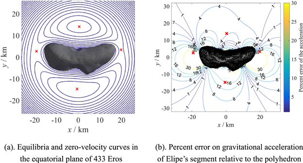
Figure 11. Equilibrium points of the asteroid 433 Eros generated by its polyhedral model and the comparison of gravitational acceleration with Elipe's massive straight segment.
Download figure:
Standard image High-resolution imageThe dipole segment model is used here to approximate the potential distribution of Eros to compare with Elipe's result (Elipe & Lara 2003) shown in Figure 11(b). Using the method in Section 4.1, the optimized parameters are μ1 = 0.429, μ2 = 0.580, and ε = 2.356, resulting in the characteristic length l of 19.851 km and κ = 0.520. Percent errors on acceleration and potential of Eros between the polyhedral model and the dipole segment are given in Figure 12, respectively. Recall from Figure 11(b) that the percent error of acceleration is about 12% at 31 km away from the origin along axis ox. Such an error has been reduced to 1% ∼ 2% for the optimized dipole segment model, and the potential error is less than 1%. Nevertheless, the acceleration errors near E1, E2, and E3 are still at the level of 10%. Compared with that of other sample asteroids like Bacchus or Hartley-2, the above errors are still too high to be a good approximation.

Figure 12. Percent errors on acceleration and potential between the dipole segment and the polyhedral model for 433 Eros.
Download figure:
Standard image High-resolution image
Due to the arc-like shape of Eros, the y coordinates of the two collinear equilibria E1 (2.648 km) and E2 (3.382 km) are far away from the axis ox, which cannot be approximated by using the axisymmetrical dipole segment. Additionally, the two triangular points are located at different sides of the axis oy. The negative x coordinate of E3 cannot be reproduced within either the dipole segment model or other traditional symmetrical simple models with μ1 ∈ [0, 0.5]. For such reasons, the dipole segment model does not seem suitable for the potential approximation of Eros-like asteroids. The dipole segment model is better adopted for the approximation of nearly axisymmetrical and elongated asteroids.