


Abstract
Residual calibration errors are difficult to predict in interferometric radio polarimetry because they depend on the observational calibration strategy employed, encompassing the Stokes vector of the calibrator and parallactic angle coverage. This work presents analytic derivations and simulations that enable examination of residual on-axis instrumental leakage and position-angle errors for a suite of calibration strategies. The focus is on arrays comprising alt-azimuth antennas with common feeds over which parallactic angle is approximately uniform. The results indicate that calibration schemes requiring parallactic angle coverage in the linear feed basis (e.g., the Atacama Large Millimeter/submillimeter Array) need only observe over 30°, beyond which no significant improvements in calibration accuracy are obtained. In the circular feed basis (e.g., the Very Large Array above 1 GHz), 30° is also appropriate when the Stokes vector of the leakage calibrator is known a priori, but this rises to 90° when the Stokes vector is unknown. These findings illustrate and quantify concepts that were previously obscure rules of thumb.
Export citation and abstract BibTeX RIS
1. Introduction
The mathematical foundations of interferometric radio polarimetry were first formulated two decades ago by Hamaker et al. (1996). Their work marked a significant improvement over the previous "black box" approach presented by Morris et al. (1964) (see also Gardner & Whiteoak 1966 for an early history of radio polarimetry). The formalism developed by Hamaker et al. (1996) continues to underpin cutting-edge developments in calibration (e.g., Smirnov 2011).
In a companion paper, Sault et al. (1996) examined the practicalities of calibrating an array in the presence of errors due to incorrect assumptions about calibrators or poorly determined parameters in the calibration process. An insightful summary of the manner in which these various influences will lead to corruption of calibration parameters was presented in Table 1 of Sault et al. (1996). However, it is not trivial to convert between the parameters presented in this seminal work and the errors implied for calibrated data because this requires taking into account the observational calibration strategy employed. An accessible overview of these errors is needed to design efficient observing schemes in the present era of increasing telescope automation. It is also needed more generally as an educational tool to foster deeper understanding of radio polarimetry.
Some efforts have been made to improve this situation, such as the investigation of dynamic range limitations presented by Sault & Perley (2014). However, other fundamental questions remain unaddressed. For example, what is the fractional polarization below which a calibrator can be assumed to be unpolarized, or what are the requirements on a calibrator's minimum coverage in parallactic angle4 throughout synthesis, to ensure that post-calibration residual instrumental polarization or position-angle errors remain below nominated thresholds?
The aim of this work is to fill the gap by presenting a practical guide to errors in interferometric radio polarimetry that explicitly accounts for calibration strategy. The structure is as follows. Section 2 presents general assumptions concerning the types of interferometric arrays and the observational parameter space that will be considered in this work. Section 3 presents a concise overview of polarization fundamentals, providing conceptual and notational context for the remaining work. Section 4 explores calibration strategies involving unpolarized and polarized calibrators, examining the roles that a calibrator's fractional polarization, signal-to-noise ratio (S/N), and parallactic angle coverage play in limiting post-calibration residual instrumental polarization. The same parameter space is explored in Section 5 but with a focus on position-angle errors. Section 6 concludes.
2. Assumptions
This work will assume an interferometric array with the following characteristics. First, all feeds are alt-azimuth (alt-az) mounted, i.e., situated on alt-az antennas without dish rotators such as those used on the Australian Square Kilometre Array Pathfinder. Second, there are at least three baselines; closure between  antennas is required to solve for of order N matrices from
  baselines (Sault et al. 1996). Third, parallactic angle (ψ) is constant across the array, within mechanical alignment errors, such that
  for all i antennas (i.e., the array is small). And fourth, all antennas are fitted with dual orthogonal linear (X, Y) or circular (R, L) feeds with the same nominal alignment, forming a homogeneous array. From these, all polarization products are measured.
Polarization calibrators will be assumed to be unresolved and located on-axis. The off-axis polarimetric response of the system will not be considered. Any frequency dependence of parameters will be assumed implicitly.
This work will focus on linear polarimetry.5 Circular polarization calibration will be touched on for completeness in Section 3, but no error analysis will be pursued (where circular to linear leakage effects, or vice versa, may be important).
Results will be illustrated for two representative arrays: the Atacama Large Millimeter/submillimeter Array (ALMA), which observes with linear feeds in all bands, and the Karl G. Jansky Very Large Array (VLA), which observes with circular feeds in all bands above 1 GHz.
Terminology and notation throughout this work will follow conventions from the widely used Common Astronomy Software Applications package (CASA; McMullin et al. 2007).
3. Polarization Fundamentals
The measurement equation for a radio interferometer (Hamaker et al. 1996; Noordam 1996; Sault et al. 1996; Smirnov 2011) relates observed visibilities to ideal model visibilities on a baseline between antennas i and j as

where the corrupting Mueller matrix terms (frequency-dependent outer products of antenna-based Jones matrices;  ) are associated from right to left with parallactic angle, instrumental polarization leakage, combined electronic and atmospheric gains, and bandpass, respectively. Some terms are neglected above for clarity (e.g., Faraday rotation and phase delay associated with the ionosphere/plasmasphere, dependence on antenna elevation, non-antenna-based terms). Calibration involves solving for these terms any applying their inverse to the observed data to recover corrected data

where antenna indices will now be omitted unless required for clarity. While the corrupting terms in the measurement equation are written as independent effects along the signal path (i.e., from right to left in Equation (1)), in general they are not independent. Care must therefore be taken to distinguish dominant terms from those that are coupled to others. The former can be solved for independently, while the latter require an iterative approach to converge on a global solution over multiple terms.6
The measurement equation is typically refactored to the relative phase frame of the bandpass/gain reference antenna (phase fixed to zero in both polarizations on this antenna):

in which the refactored terms are identified by subscript r, the crosshand bandpass phase7
on the reference antenna  that arises from the refactoring of
  remains unconstrained,
  is separated into crosshand delay
  and crosshand phase
  terms that capture first-order linear and residual nonlinear frequency dependence, respectively, and leakages
  are measured in the crosshand phase frame.8
The leakage terms ("dipole" terms or d-terms) describe imperfections in the polarimetric response of the system and quantify the degree to which each feed is sensitive to an orthogonally polarized signal. The imperfections arise from both telescope geometry (e.g., antenna illumination, feed horn, optics alignment) and electronic hardware (e.g., polarization splitter, hybrid coupler). Notation for leakages in this work will follow the Jones matrix form:
for antenna i where p is given by X (linear basis) or R (circular basis), dpi is the fraction of the q (orthogonal) polarization sensed by p, and on-diagonal effects are factored into  and
and  (Sault et al. 1996).9
Frequency dependence (ν) will be assumed implicitly throughout this work and omitted below. Other terms from the measurement equation that are most relevant to this work are parallactic angle in the linear feed (LF) and circular feed (CF) bases and crosshand phase on the reference antenna. These take the respective Jones forms
(Sault et al. 1996).9
Frequency dependence (ν) will be assumed implicitly throughout this work and omitted below. Other terms from the measurement equation that are most relevant to this work are parallactic angle in the linear feed (LF) and circular feed (CF) bases and crosshand phase on the reference antenna. These take the respective Jones forms
and
where ψ is parallactic angle, and
where ρ is crosshand phase.
For an interferometer with dual linearly polarized feeds,  is given by the four-element vector


whereas for circular feeds the vector is


The model visibilities for a single baseline, corrupted by parallactic angle, leakage, and crosshand phase terms ( ), are given in the linear basis by


where  ,
,  , and terms multiplied by second-order leakages (e.g.,
  ) are neglected. The visibilities in the circular basis are given by
Analysis in this work will be restricted to the linearized equations presented above (first order in d-terms). Furthermore, polarization calibration will be limited to examination of crosshand visibilities only, with the additional assumption that Stokes  is zero (unless a nonzero model is available). These simplifications are currently used within CASA and are suitable for the focus on linear polarization in this work (note that the full quadratic approach is used in other packages such as MIRIAD; Sault et al. 1995).
Crosshand phase calibration can be performed (e.g., in CASA) by taking the average over all baselines for the sum of crosshand visibilities,
In the circular basis, when leakages are known, crosshand phase calibration is synonymous with calibration of the absolute alignment of linear polarization10
and requires an external source of known position angle. In the linear basis, an offset in the absolute alignment of the feeds (i.e., different observed  and
and  in Equation (24)) does not translate into a trivial change in crosshand phase. Thus, in the linear basis, crosshand phase and absolute position-angle calibrations are not synonymous. However, unlike in the circular basis, if the linear antenna feeds are nominally aligned to the sky, an external source of known position angle is not formally required; variation in
  over parallactic angle for a linearly polarized source with unknown
  and
and  is sufficient to solve for ρ. As a result, calibration strategies in the linear basis typically need to obtain a first-pass solution for
  , assuming zero leakages, prior to solving for
  . Subsequent iteration is technically required (though typically negligible in practice) to account for leakages in the solution for
  . In the circular basis,
  is not needed to solve for the leakages (crosshand phase simply imparts an overall rotational ambiguity) while
  is needed to optimally solve for
  . Thus circular basis calibration strategies typically solve for
  prior to
  .
.
Figures 1 and 2 illustrate how the respective corrupted cross hands from Equations (17) and (21) trace out geometric features in the complex plane as a function of parallactic angle coverage. In the linear basis,  moves along a rotated linear axis that is offset from the origin by leakages and broadened to become an ellipse due to the product of leakages with
  . In the circular basis, a circle is drawn with center offset by the leakages (e.g., Conway & Kronberg 1969). These figures highlight degrees of freedom that must be calibrated. For example, calibration strategies in the circular basis that involve a polarized calibrator with unknown Stokes vector require at least three independent observations to solve for the d-terms (provided there are at least three baselines) as well as Stokes
  and
and  . Geometrically, this can be viewed as the need for three points to solve for the unknown origin and radius of a circle. When the Stokes vector is known a priori, only two observations are required to locate the origin (the known sense of rotation between the observations breaks the origin degeneracy). Degrees of freedom are examined more formally in the following section.
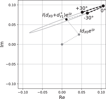
Figure 1. Path traced in the complex plane by corrupted VXY from Equation (17) on a single baseline (i = 0, j = 1) for a calibrator with  , instrumental leakages dX0 and dY1 with moduli 0.05 and respective phases 10° and
  , and crosshand phase
  . The ellipse indicates the path traced by complete parallactic angle coverage, while the dashed curve indicates the path traced from
  to
to  through 0°. The lighter-shaded dashed line connects the center of the ellipse to
  . The lighter-shaded dotted lines and points indicate how leakage from total intensity offsets the center of the ellipse from zero.
Download figure:
Standard image High-resolution image
Figure 2. Path traced in the complex plane by corrupted VRL from Equation (21) for a single baseline. All calibrator and instrumental parameters are the same as described for Figure 1, but with leakage subscripts X and Y replaced by R and L, respectively. Full parallactic angle coverage traces a circle, offset from zero by leakage from total intensity.
Download figure:
Standard image High-resolution image3.1. Degrees of Freedom
Polarimetric calibration involves solving for the crosshand phase, leakage d-terms, and absolute alignment of linear polarization. External calibration is required to determine the absolute position angle in the same way that an interferometer cannot self-calibrate the absolute flux density level. Theoretically, to solve for all degrees of freedom in any basis that uses dual orthogonally polarized feeds, at least three distinct observations of calibrators with linearly independent Stokes vectors are required (Sault et al. 1996). This implies that at least two observations need to be on a polarized calibrator, at least one needs to be linearly polarized, and a circularly polarized calibrator is not essential. Observation of a linearly polarized calibrator over a range of parallactic angles can provide the necessary three distinct observations; rotation of the sky within the alt-az instrument frame enables the leakages and source polarization to be jointly solved. In practice, for circular polarization science in the linear feed basis, external (absolute) calibration of Stokes  is also required11
(e.g., Rayner et al. 2000), due to leakages being small (as a result of good engineering).
is also required11
(e.g., Rayner et al. 2000), due to leakages being small (as a result of good engineering).
3.2. Absolute versus Relative Leakages
Observational constraints may not always be available to solve for the d-terms unambiguously. For example, an unpolarized calibrator will yield solutions that are degenerate in the sum of leakage pairs, e.g.,  . This corresponds to an undetermined Jones matrix which, in the small-angle approximation, corresponds to a complex offset (β) that can be added to one polarization and subtracted with conjugation from the other, e.g.,
  and
and  for all antennas (Sault et al. 1996). When solving for degenerate leakages, the real and imaginary components of the X or R feed leakages will be (arbitrarily) set to a constant (typically zero) on the gain reference antenna, effectively setting β to the negative of the true d-term on this antenna (e.g.,
  ). Leakage solutions degenerate in this manner are known as relative leakages. Absolute leakages are accessible only when additional observational constraints are available, e.g., from multiple observations of a polarized calibrator.
Relative leakages cannot replace absolute leakages in the measurement equation without incurring errors. For calibration strategies that recover relative leakages, the degenerate nature of the solutions will manifest in the linear basis as an error in the position angle of linear polarization, an unknown degree of leakage between linearly and circularly polarized components, and gain errors in total intensity. In the circular basis there will be an unknown degree of leakage between linearly and circularly polarized components and gain errors will be produced in total intensity (Sault et al. 1996, or glean from equations presented in Section 3). As described earlier, this work will focus only on leakages accessible through the linearized crosshand visibilities. Accordingly, calibration strategies in the linear feed basis may recover relative or absolute leakages, depending on available observational constraints. Absolute leakages are accessible because the d-term sum degeneracy can be broken purely in the cross hands by  . Leakages in the circular basis, however, will always be relative; absolute leakages cannot be easily recovered without accessing the quadratic terms in the parallel-hand visibilities or performing observations in which a subset of receivers are physically rotated (Sault & Perley 2013).
For completeness, it is worth noting that absolute leakages will often be quasi-absolute in practice because the measurement equation formalism assumes that the full signal path is characterized by a specific and limited set of effects. For example, the measurement equation under consideration may neglect terms regarding analogue components of the telescope (Price & Smirnov 2015) or direction-dependent effects (Smirnov 2011). In practice, absolute leakages are non-singular solutions within the assumed framework.
4. Residual on-axis Instrumental Polarization
Strategies to calibrate instrumental leakage typically involve a single observation of an unpolarized calibrator, or multiple observations of a polarized calibrator spanning a range of parallactic angles. This section will present results from analytic derivations and Monte Carlo simulations with the aim of elucidating calibrator requirements so that subsequent observation of an unpolarized science target will deliver spurious on-axis polarization below a nominated threshold. For example, ALMA specifications require residual instrumental on-axis polarization to be below 0.1% of total intensity after calibration. Sections 4.1 and 4.2 will examine unpolarized and polarized calibrators, respectively, in both the linear and circular feed bases.
Throughout the following, an observation of a calibrator at a particular parallactic angle will be termed a slice. A slice may comprise one or more observational scans (in VLA parlance), but it will be assumed that parallactic angle is approximately constant throughout the slice and that the quoted S/N represents all combined scans within the slice. Note that, in practice, these concepts are linked: the ability to define the timespan over which parallactic angle can be considered constant is a function of S/N. Separation of these concepts is useful for framing the simulations. However, caution is required to ensure that parallactic angle variation within the time needed to obtain a requisite S/N is not comparable to the parallactic angle range over which significant changes in residual leakage are predicted to occur.
A requirement for maximum spurious on-axis polarization translates to a calibration requirement for d-term accuracy. Taking  as the characteristic d-term modulus error12
and Na as the number of antennas in the array, the approximate level of spurious on-axis linear (
as the characteristic d-term modulus error12
and Na as the number of antennas in the array, the approximate level of spurious on-axis linear ( ) or circular (
 ) polarization produced when observing an unpolarized source in the linear feed basis is

Spurious elliptical polarization is

In the circular feed basis, the level of spurious linear or elliptical polarization is

No spurious circular polarization will be produced. Analytic derivations of these equations are presented in the Appendix. To illustrate, a requirement of 0.1% spurious on-axis linear polarization translates to  ≲ 0.6% for ALMA (Na = 40) and
  ≲ 0.4% for the VLA (Na = 27). The equations above assume a worst-case scenario where the science target is observed within a single parallactic angle slice. For wider parallactic angle coverage the residual leakage will be smaller due to depolarization.
The equations above will now be used to translate  into limits on anticipated spurious on-axis polarization for various calibration strategies.
4.1. Unpolarized Calibrators
A calibrator that is classified as unpolarized may in fact exhibit a low level of polarization, denoted by  ,
,  , or
, or  (other terms not needed below). Taking this into account, if leakage calibration is performed using an assumed unpolarized calibrator (resulting in relative leakages), the resulting d-term modulus error
  will be approximately
in the linear feed basis and
in the circular feed basis, where A is the full-array dual-polarization total intensity S/N of the calibrator within the single spectral channel of interest. Derivations of these equations are presented in the Appendix. Note that the level of fractional polarization below which a source may be classified as "unpolarized" depends on the telescope being used and the science goals of the observation. For science projects or telescopes that place a requirement on the acceptable level of spurious on-axis polarization following calibration, the equations above can be used to determine whether a calibrator can be classed as unpolarized. Note that the limitations on dynamic range arising from errors in the calibrator model presented by Sault & Perley (2014) may be relevant or may even dominate considerations for some science goals.
Leakage calibration with an unpolarized calibrator can be performed using a single-slice observation. In the circular basis, taking an example of an assumed unpolarized calibrator with true linear polarization  observed with the VLA at high S/N, the estimate from Equation (30) is
  . The estimated spurious on-axis fractional polarization for an unpolarized science target observed over a small range in parallactic angle (e.g., snapshot) is then
  from Equation (28). As another example, now in the linear basis using an unpolarized (or negligibly polarized) calibrator, the estimated spurious fractional linear polarization for an unpolarized science target is
  .
.
4.2. Polarized Calibrators
4.2.1. Linear Basis
To calibrate leakages in the linear basis using a polarized source, observations are required over at least three parallactic angle slices if the Stokes vector is unknown a priori, or as little as a single slice if the Stokes vector is known. When the Stokes vector is unknown a priori, it needs to be solved for in addition to the d-terms and crosshand phase. For the case of a single-slice observation on a calibrator with known Stokes vector, the available degrees of freedom only permit solving for relative leakages. In all other calibration strategies, absolute leakages can be recovered.
Simulations were performed to predict the level of spurious on-axis polarization and absolute position-angle error resulting from a strategy involving one slice (linearly polarized with Stokes known), two (linearly polarized with Stokes known), three (Stokes unknown), and ten (Stokes unknown). Full details are presented in the Appendix, including a web link to the simulation code, which has been made publicly available. This section will present the results for spurious polarization. Position-angle errors will be reported in Section 5.1.
The simulations explore the accuracy with which the d-terms, crosshand phase, and calibrator polarization (when relevant) can be measured from the crosshand visibilities when a source is subjected to parallactic angle rotation in the presence of thermal noise. To solve for  , the code focuses on a single cross product (VXY) and examines how well the d-term for the antenna and polarization under consideration can be recovered while taking into account all available
  baselines toward antenna i. The simulations assume an ALMA-like array with 40 antennas, typical d-term modulus of 1.5%, and uncertainty in mechanical feed alignment of 2° per antenna (Cortes et al. 2015); the uncertainty in alignment is only used for analysis of position angle (see Section 5.1).
For multislice strategies, the first slice is assumed to be observed at maximum  . This produces approximately worst-case results, compared to, for example, symmetric coverage about maximum
  , because the arc traced along the ellipse in the complex plane for a crosshand visibility is minimized, leading to poorer constraints on recovered parameters. Note that truly worst-case results would arise from limited coverage about
  , in which case crosshand phase would be degenerate and calibration would fail. The simulations use Monte Carlo sampling to recover the distribution of
  , from which the 95th percentile is measured and converted to spurious linear polarization using Equation (26). Two scenarios have been examined, the first for a calibrator exhibiting 3% fractional linear polarization and the second with a fraction of 10%.
Results for the one-slice strategy are presented in Figure 3. The displayed trend in spurious fractional polarization is practically indistinguishable from the analytic prediction for an unpolarized calibrator described at the end of Section 4.1. The reason is because d-term errors arising from crosshand phase errors, drawn from data where all baselines are combined in the solution, always remain practically negligible compared to thermal noise in the subset of baselines from which individual d-terms are effectively solved. Thus the fractional polarization of the calibrator will not practically affect the result (unless it approaches 100%); curves obtained for the 3% and 10% fractionally polarized cases are indistinguishable.
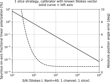
Figure 3. Results from simulations showing 95th percentile spurious on-axis fractional linear polarization and absolute position-angle error, predicted to arise within one spectral channel when a linear basis telescope is calibrated using a single-slice observation of a polarized calibrator with known Stokes vector. The indicated position-angle error must be added in quadrature with a target source's statistical error to obtain its total position-angle error. The displayed curves are from simulations with a 3% linearly polarized calibrator. Results from the 10% case are not displayed because they are indistinguishable.
Download figure:
Standard image High-resolution imageResults for the strategies involving two, three, and ten slices are displayed in Figure 4. The distorted contours seen at very small or very large parallactic angle coverages in panels where the Stokes vector is unknown are artifacts that can be ignored; these are the result of simplifications in the code that are localized to these regions of parameter space (the temporal ordering of points is ignored). The plots indicate that, in general for a given calibrator, total parallactic angle coverage of approximately 30° is sufficient to maximize calibration accuracy. Beyond 30°, additional parallactic angle coverage delivers only minor improvements. In the two-slice strategy, separation of slices beyond approximately 70° will lead to degraded calibration solutions and increased spurious polarization. The levels of spurious polarization are found to be smaller when using a more highly fractionally polarized calibrator, as expected.
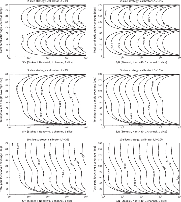
Figure 4. Results from simulations showing 95th percentile spurious on-axis fractional linear polarization (per cent) for an unpolarized target arising from different calibration strategies with a linear basis telescope. The simulations assume an ALMA-like array with 40 antennas. Top row: two-slice strategy with polarization known a priori. Middle row: three-slice strategy with unknown polarization. Bottom row: ten-slice strategy with unknown polarization. Panels in the left and right columns show results obtained using a calibrator with 3% or 10% fractional linear polarization, respectively. Abscissa: full-array dual-polarization total intensity S/N within one spectral channel and one slice. Ordinate: total parallactic angle coverage; divide by one less than the number of slices to get the interslice separation. The distorted contours seen at very small and very large parallactic angle coverages in some panels are the result of coding artifacts and should be ignored.
Download figure:
Standard image High-resolution image4.2.2. Circular Basis
To calibrate leakages in the circular basis using a polarized source, observations are required over at least two or three parallactic angle slices, depending on whether the Stokes vector is known a priori or not, respectively. When unknown a priori, the Stokes vector needs to be solved for in addition to the d-terms.
Monte Carlo simulations similar to those described for the linear basis were performed to predict the level of spurious on-axis polarization and absolute position-angle error resulting from a strategy involving two slices (linearly polarized with Stokes known), three (Stokes unknown), and ten (Stokes unknown). To solve for  , the code focuses on a single cross product (VRL) and examines how well the d-term for the antenna and polarization under consideration can be recovered while taking into account all available
  baselines toward antenna i. The simulations assume a VLA-like array with 27 antennas. Full details are presented in the Appendix, including a web link to the publicly available simulation code. This section will present the results for spurious polarization, which is calculated in the code by taking the recovered 95th percentile
  and performing a conversion using Equation (28). Position-angle errors will be reported in Section 5.2.
Results are displayed in Figure 5. The distorted contours seen at small parallactic angle coverages in panels where the Stokes vector is unknown are artifacts that can be ignored; they are the result of simplifications in the code that are localized to these regions of parameter space (the temporal ordering of points is ignored). The plots demonstrate that, as expected, a floor is reached at low S/N where no amount of parallactic angle coverage can make up for the dominant randomizing influence of thermal noise. This is not seen in the linear basis results because the method of solving for the d-terms is different (see Appendix; linear basis calibration can take advantage of prior crosshand phase calibration). Note that the displayed range of S/N differs between the linear and circular basis plots.
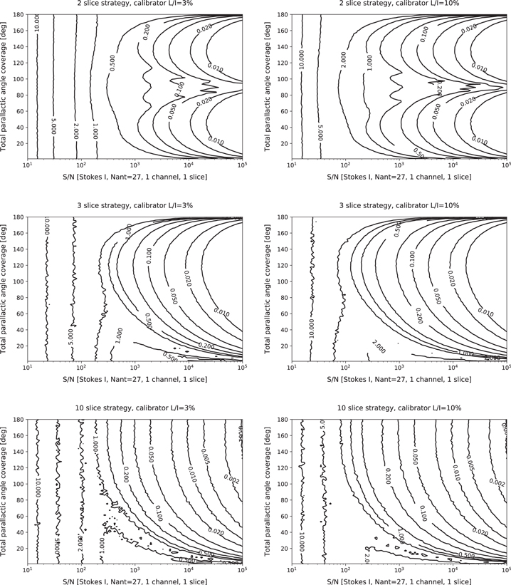
Figure 5. Results from simulations showing 95th percentile spurious on-axis fractional linear polarization (per cent) for an unpolarized target arising from different calibration strategies with a circular basis telescope. The simulations assume a VLA-like array with 27 antennas. Panel layout and axes are the same as in Figure 4. The distorted contours seen at small parallactic angle coverages in some panels, in which a valley is produced, are the result of coding artifacts and should be ignored.
Download figure:
Standard image High-resolution imageThe two-slice strategy reveals the counterintuitive result that a calibrator with larger fractional polarization will, at low S/N, result in higher spurious polarization than a calibrator with low fractional polarization. This is because the fractional polarization is a fixed known quantity when S/N is defined for total intensity; solving for the origin of a circle with fixed radius in the presence of thermal noise leads to larger fractional errors when the radius is larger. Indeed, this trend continues to the case of unpolarized calibrators; spurious polarization limits are even smaller when observing an unpolarized calibrator at the equivalent S/N. For the three- and ten-slice strategies, the Stokes vector is not known a priori, so calibrators with higher fractional polarization deliver better quality solutions than calibrators with lower values, as expected.
The results presented here indicate that, in general, when the Stokes vector of the leakage calibrator is known a priori, total parallactic angle coverage of approximately 30° is sufficient to maximize calibration accuracy. Additional coverage is not found to deliver significant improvements. In the two-slice strategy, separation of slices beyond approximately 70° will lead to degraded calibration solutions and increased spurious polarization. These match findings for the linear basis presented in Section 4.2.1. However, when the Stokes vector is unknown in the circular basis, the minimum coverage requirement increases to approximately 90°.
5. Position-angle Errors
As with leakage calibration, observational constraints may not always be available to perform absolute position-angle calibration. If absolute position angles are not calibrated, scientifically useful data may still result, for example if the spectrum of fractional polarization is of interest, or in particular for the linear basis if position angles are only partially calibrated. The following sections explore position-angle errors in the linear and circular bases.
5.1. Linear Basis
In the linear basis, calibration strategies must recover  , the real part of the d-term on the X feed of the gain reference antenna, in order to provide self-consistent alignment to the assumed sky frame. If relative leakages are recovered, a systematic contribution to position-angle errors will be imposed, given by the magnitude of
  . For example,
  implies a systematic contribution from position-angle error of
  . This relationship can be derived by considering how the unaccounted degree of freedom associated with the true value of
  will be absorbed by
  and
and  in Equations (16)–(19) when relative leakages (r) are utilized, compared with their original values calculated in the presence of absolute leakages (a). The differences are
  and
and  . The difference in position angle is then
  in the small-angle approximation.
The above calculation can also be used to estimate position-angle errors resulting from d-term statistical measurement errors. The resulting worst-case position-angle error is approximately  , i.e., if all d-terms were made relative to an offset of this magnitude.
An additional systematic position-angle error will arise due to each antenna in the array exhibiting a nonzero uncertainty in mechanical feed alignment about the nominal alignment (where the nominal alignment is a specified angle between the X feed and the meridian at  ). Thus, in general, the standard error in the mean of feed alignments over the array will be nonzero, leading to an offset between the assumed and true sky frames. In turn, measured Stokes
  and
and  will be slightly rotated versions of their true values. Leakage calibration will remain internally consistent for both relative and absolute cases, accounting for the misaligned feeds. However, the systematic misalignment over the array will remain uncorrected. External position-angle calibration, using a source with known Stokes vector to adjust
  and perform relative application to all other leakages, is required to account for this offset and provide true absolute position-angle calibration. For statistically independent feed misalignments over the array (not necessarily true in practice due to correlated installation procedures), the systematic contribution from position-angle uncertainty will be approximately
  , where ϕ is the characteristic uncertainty in alignment per antenna. To illustrate, this is ≲
  for ALMA.
Thus, total systematic position-angle uncertainty (i.e., frame error) for a target source in the linear basis is the quadrature sum of up to three terms: systematic error when relative leakages are recovered (i.e., when  is artificially set to complex zero) given by the magnitude of the true
  , systematic error from d-term measurement errors, and systematic feed misalignment error. The relationship is
Total position-angle error can then be calculated for a target source by combining the total systematic error above with statistical error (i.e., in-frame error) associated with the S/N of detection.
In this section, and in the simulation code developed for this work, it will be assumed that linear basis calibration does not include absolute position-angle calibration (i.e., the final term in Equation (31) will be included in all calculations). This is regardless of whether relative or absolute leakages are recovered, or importantly whether a linearly polarized calibrator with known Stokes vector is available or not. This is consistent with typical data reduction procedures for major telescopes such as ALMA and the Australia Telescope Compact Array (ATCA). Results for position-angle errors can therefore be compared directly between the calibration strategies examined in this work. To include the effect of absolute position-angle calibration in any of the results, subtract  in quadrature, where
  is the value assumed in the simulations. Systematic position-angle errors resulting from the use of unpolarized and polarized calibrators will now be examined.
If an unpolarized calibrator is utilized for polarization calibration, relative leakages will be recovered. The total systematic position-angle error is then estimated using Equation (31), including the first term. A worst-case estimate for the second term is given by  from Equation (29).
Position-angle errors arising from calibration strategies involving a polarized calibrator were examined using the Monte Carlo simulations involving one, two, three, and ten slices introduced in Section 4.2.1. Position-angle errors were calculated in a similar manner to leakages, taking the recovered 95th percentile  from the simulations and evaluating the total systematic position-angle error using Equation (31). The first term in Equation (31) was included only for the one-slice simulation; the other calibration strategies recover absolute leakages.
The result from the one-slice simulation is displayed in Figure 3. The asymptotic behavior is due to the final term in Equation (31). As with the curve for spurious leakage, the overall curve for position-angle error is practically indistinguishable from the analytic prediction for an unpolarized calibrator that may be obtained by combining Equation (29) with Equation (31).
Results from the two-, three-, and ten-slice strategies are displayed in Figure 6. Similar conclusions regarding parallactic angle coverage may be drawn as for leakages described in Section 4.2.1.
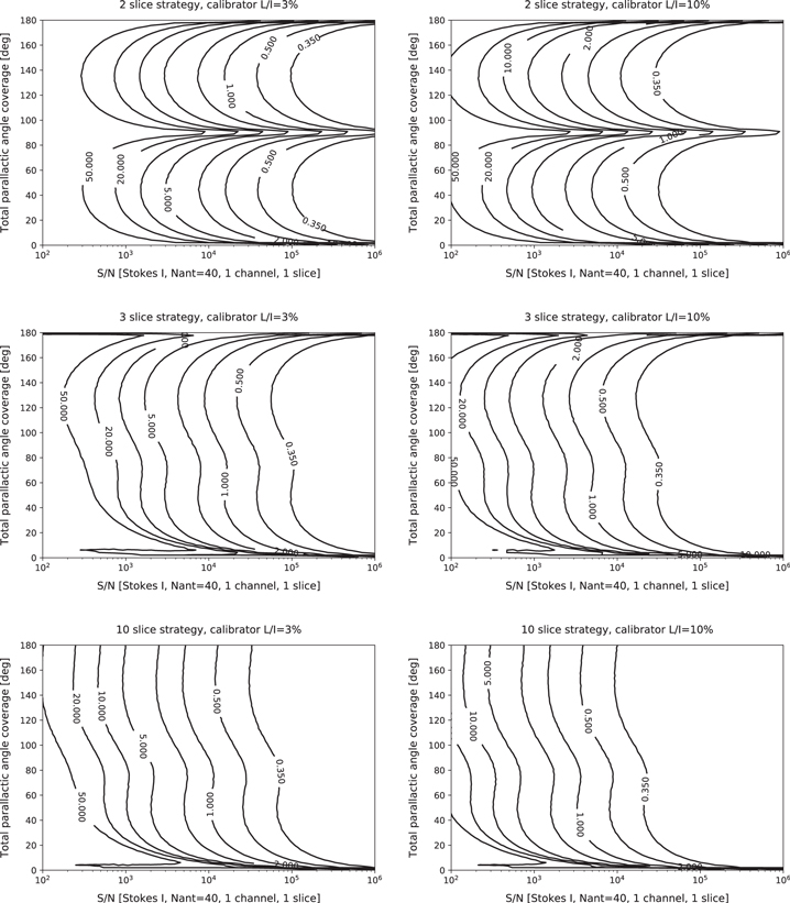
Figure 6. Results from simulations showing 95th percentile systematic position-angle error (degrees) arising from different calibration strategies with a linear basis telescope. Panel layout and axes are the same as in Figure 4. The distorted contours seen at very small and very large parallactic angle coverages in some panels are the result of coding artifacts and should be ignored.
Download figure:
Standard image High-resolution image5.2. Circular Basis
Position-angle calibration in the circular basis is tied to crosshand phase calibration. This requires a polarized calibrator.
To examine position-angle errors resulting from crosshand phase calibration, a Monte Carlo simulation was performed based on Equation (25). The result is presented in Figure 7. To illustrate interpretation of this figure, consider position-angle calibration with the VLA within a 2 MHz channel at 3 GHz using 3C48 (∼10 Jy, ∼2% fractional linear polarization). An S/N in excess of 300 is required to limit systematic position-angle uncertainty to within  . This translates to an on-source time approaching 4 minutes. For
  uncertainty, the required on-source time is ∼30 s.
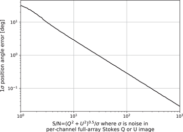
Figure 7. Result from simulation showing systematic position-angle error for calibration with a circular basis telescope. Abscissa: full-array dual-polarization linear polarization S/N within one spectral channel. Ordinate: standard error in systematic position-angle error.
Download figure:
Standard image High-resolution image6. Conclusions
The mathematical framework for describing interferometric radio polarimetry does not readily permit quantitative calculation of post-calibration residuals for specific observational calibration strategies. This work has bridged this gap through the presentation of analytic derivations and results from Monte Carlo simulations. In general, worst-case errors have been assumed. Thus, in practice, residual leakage and position-angle errors are likely to be smaller.
This work has focused on arrays that comprise alt-az antennas with common feeds over which parallactic angle is approximately uniform, such as ALMA and the VLA. The simulation code has been made publicly available to support potential extension, for example to investigate mixed basis arrays (e.g., Martí-Vidal et al. 2016), very long baseline interferometry, calibration strategies using resolved polarization calibrators, or a more detailed examination of circular polarimetry.
This work was motivated by the need to implement automated polarization data reduction capabilities within the CASA integrated pipelines for ALMA13 and the VLA.14 As a result, this work forms part of ALMA Memo 603, equivalently referenced as EVLA Memo 201 (Hales 2017b). This memo contains extensive additional material, including a general classification system for polarization calibrators, and detailed step-by-step procedures for performing a suite of polarimetric calibration strategies in the linear and circular bases.
I thank the following for insightful discussions: George Moellenbrock, Bob Sault, Brian Kent, Lindsey Davis, Vincent Geers, Kumar Golap, Jeff Kern, Joe Masters, and Claire Chandler. I thank the ALMA Integrated Science Team for reviewing this document under the context of CASA automated pipeline design. I thank the anonymous referee for their thoughtful review, which led to the improvement of this paper. The National Radio Astronomy Observatory is a facility of the National Science Foundation operated under cooperative agreement by Associated Universities, Inc. This project has received funding from the European Union's Horizon 2020 research and innovation programme under the Marie Skłodowska-Curie grant agreement No 705332.
Software: Simulation code (Hales 2017a), CASA (McMullin et al. 2007).
Appendix: Residual on-axis Instrumental Leakage
Section 4 presented equations to predict the level of spurious on-axis polarization that will be observed for an intrinsically unpolarized target source following the application of imperfect d-term calibration solutions. Using these relationships, Section 4.1 presented equations to predict the d-term measurement errors, and in turn the level of spurious polarization, that will result following leakage calibration when using a polarized calibrator that is assumed to be unpolarized. Similarly, Section 4.2 presented results from simulations in which d-term measurement errors, and ultimately spurious polarization signatures, were predicted empirically for calibration schemes involving observation of a polarized calibrator over a range of parallactic angles (slices). Derivations for all equations, and details of the simulations, are presented below for the circular and linear feed bases.
A.1. Circular Basis
Stokes  is formed by

If d-terms are recovered with measurement errors  (statistical or systematic in origin), an unpolarized target will be observed with spurious fractional polarization

The worst-case spurious polarization will therefore occur for a target observed with limited parallactic angle coverage. If the science target is integrated over a wide range in parallactic angle, then the level of spurious polarization predicted in the following should be treated as an upper limit. Taking the worst-case scenario of approximately constant parallactic angle, and noting that there are only Na independent d-terms per polarization over the array, the relationship above can be rewritten in a statistical sense as
For characteristic d-term modulus error  , the variance in
 ![$\mathrm{Re}[{\rm{\Delta }}d]$](https://content.cld.iop.org/journals/1538-3881/154/2/54/revision1/ajaa7aefieqn108.gif) is given by
is given by  . The variance in Equation (34) is then estimated as
Similar analysis for fractional  yields the same result. The predicted level of spurious on-axis fractional linear polarization is then Rayleigh distributed with mean
No spurious circular polarization is predicted ( ) because its evaluation does not include any leakage products with total intensity (to first order). The results above are presented in Section 4.
If a polarized calibrator is assumed to be unpolarized for leakage calibration, any true (linear) polarization will lead to corruption of the measured leakages. The difference between observed and true crosshand visibilities for a single baseline is given by

Note that nonzero  will not affect relative leakages that are calculated using only crosshand data (to first order). The equation above is effectively constrained by
  baselines toward antenna i, in which case
In this construction, the leakages will soak up the source polarization, leaving the  term consisting of only thermal noise. As a result, its average on the right side of the equation can be represented by a vector with characteristic magnitude
  , where A is the full-array dual-polarization total intensity S/N of the calibrator within the single spectral channel of interest. The first term on the left side of the equation has characteristic magnitude
  . The importance of the next term, containing the average over d-terms, depends on whether the d-terms are correlated between antennas or not. When random errors dominate over systematics from the true source polarization (e.g., for small A), the recovered d-term errors will be effectively uncorrelated. In this case, the term can be viewed as a vector-averaged sample of (
 -scale) error vectors, in which case its contribution will be negligible15
and can be ignored. When source polarization systematics dominate (e.g., for large A), the d-terms will be correlated and the average cannot be ignored. This can be crudely accommodated by replacing
-scale) error vectors, in which case its contribution will be negligible15
and can be ignored. When source polarization systematics dominate (e.g., for large A), the d-terms will be correlated and the average cannot be ignored. This can be crudely accommodated by replacing  with
with  , in which case the left side of Equation (38) can be approximated by
  . Thus, the estimated
  will be half of the value recovered when assuming uncorrelated d-terms. Given the simplistic nature of this calculation, the larger estimate for
  will be adopted; its estimated value presented below should therefore be treated as an upper limit.
By noting that contributions to  on the right side of Equation (38) represent projections onto a 1D vector given by the true d-term (requiring adjustment to variances by a factor 1/2), and by treating the true polarization as a DC offset with magnitude
  , the d-term modulus error can be estimated in rms fashion as
The resulting estimate for spurious fractional linear polarization is then obtained using Equation (36), giving
These results are reported in Section 4.1. Note that if the leakage calibrator is observed over a wide range in parallactic angle (atypical for an assumed unpolarized calibrator), then the predicted spurious polarization should be treated as an upper limit (in addition to the motivation described earlier).
Figure 5 presents estimates of spurious polarization for calibration strategies involving parallactic angle coverage of a polarized leakage calibrator. To obtain these results, a Monte Carlo simulation code was developed to estimate  and perform conversion using Equation (36). The code focuses on the theoretical aspects discussed in this document by approximating the behavior of the generalized solvers that exist within software such as CASA, as described below. Full CASA-based (or other package) simulations using mock or real data were not considered for this work because of the potential for introducing a host of unwanted systematics, which could readily bias interpretation of the fundamental attributes under investigation. The simulation code is publicly available at https://github.com/chrishales/polcalerrsims (Hales 2017a).
To estimate  for the calibration schemes examined, the code performs Monte Carlo sampling and examines the distribution of errors recovered when attempting to solve for the d-term for a single polarization on a single antenna. To do this, the code focuses on a single cross product (e.g., VRL) and examines how well the d-term under consideration can be recovered while taking into account all available
  baselines toward antenna i. The relevant relationship is given by Equation (38), with the sum over
  assumed to be negligible. The true source polarization is injected with the appropriate thermal noise at slices that are, for simplicity, spaced equally over the total parallactic angle span under consideration.
Calibration strategies involving a polarized calibrator with unknown Stokes vector require at least three statistically independent slices to solve for the d-term (error) as well as Stokes  and
and  . Geometrically, this can be viewed as the need for three points to solve for the unknown origin and radius of a circle (see Figure 2). When the Stokes vector is known a priori, only two slices are required to locate the origin (the origin degeneracy is broken by the known sense of rotation between the slices). For simplicity, the simulation code does not take into account the sense of rotation between points. As a result, the portion of parameter space containing observations at modest S/Ns over small total parallactic angle ranges displays much noisier solutions than those likely to be recovered in production code. This effect is not significant; results throughout the remaining parameter space are not affected.
The code recovers the distribution of d-term errors for each sampled point in the S/N and the parameter space of parallactic angle coverage. Rather than reporting the mean of this distribution to represent  , the code reports the 95th percentile in order to better accommodate the slightly non-Gaussian nature of the results in a conservative manner. This is consistent with the comments earlier to interpret results as upper limits.
A.2. Linear Basis
Assuming perfect crosshand phase measurement,  is formed by

The presence of d-term measurement errors will cause an unpolarized target to exhibit spurious fractional linear polarization, described statistically as
The worst-case spurious polarization will occur for a target observed with limited parallactic angle coverage. Assuming the worst-case scenario of approximately constant parallactic angle, the variance in Equation (42) is then estimated as
Similar analysis for fractional  yields the same result. No spurious
  will be produced because its evaluation does not include any leakage products with total intensity. As a result, the predicted level of spurious on-axis fractional linear or circular polarization is given by
The predicted level of spurious fractional elliptical polarization is then Rayleigh distributed with mean

These results are presented in Section 4.
The results presented in Section 4.1 regarding calibration with a polarized yet assumed unpolarized calibrator can be derived in the same way as presented earlier for the circular feed basis, but replacing  with
with  in Equation (39). For the linear basis derivation here, it will be assumed that the product of
  with leakages in the crosshand visibilities is always negligible. This will not always be true in practice, but in such cases the contribution from thermal noise (A) is likely to dominate. The resulting estimates of spurious fractional linear or circular polarization are then obtained using Equation (44), giving
The estimate of spurious fractional elliptical polarization is obtained using Equation (45), giving
Figure 4 presents estimates of spurious polarization for calibration strategies involving parallactic angle coverage of a polarized leakage calibrator. To obtain these results, simulation code was developed with similar characteristics to those described earlier for the circular feed basis. Differences are described below. The simulation code is publicly available at https://github.com/chrishales/polcalerrsims (Hales 2017a).
The code focuses on a single cross product (e.g., VXY) and examines how well the d-term for the antenna and polarization under consideration can be recovered while taking into account all available  baselines toward antenna i. Unlike in the circular basis, measurement of the crosshand phase is required here prior to solving for leakages. The linear basis simulation code therefore takes into account crosshand phase measurement errors due to thermal noise when calculating the d-term measurement errors. The code does not account for errors in crosshand phase measurement due to the as-yet unknown leakages, which are assumed to be zero for this calculation (such errors are typically negligible in the baseline-averaged crosshand phase solution, minimizing the need for iteration). The code assumes that Stokes
  is zero for all calibrators. The relevant equation is then a modified version of Equation (17),
in which thermal noise in VXY is explicitly included, denoted by  . For all multislice observing strategies, the simulation code assigns each of the d-terms that appear in the equation above with a user-defined characteristic amplitude and random phase. The error in recovering the input dXi is then ultimately recorded.
For simplicity, the code assumes that the first observed slice for each calibration strategy is at zero parallactic angle, and that the calibrator's position angle is 45°. These initial conditions should generate generally representative results for the one- and two-slice strategies, where the calibrator's Stokes vector is known a priori and may therefore be targeted appropriately by observers. However, note that the initial conditions above (or any others) cannot fully represent all possible observing configurations for the three- and ten-slice strategies, where the Stokes vector is unknown a priori. It is of course possible that rare specific configurations of these strategies could produce significantly different results than presented. It is worth noting here that when users in the linear feed basis are advised to maximize parallactic angle coverage, this really means they should maximize coverage for  (i.e., maximum arc length traced along the ellipse for a crosshand visibility). For a calibrator with unknown Stokes vector observed over as few as three slices, the difference in rare circumstances could be noticeable.
For the one-slice strategy, the simulation code measures crosshand phase error by solving for a position angle in the noisy frame indicated by Equation (24) (i.e., Xf solve in CASA terminology). For the two-slice strategy, the code performs this step using the slice with maximum  (known a priori). For the three- and ten-slice strategies, the code measures crosshand phase error by solving for a linear slope with unconstrained offset, followed by a least-squares fit to measure Stokes
  and
and  along this slope given the noisy observed variations of
  (i.e., XYf+QUf solve in CASA terminology).
For the multislice strategies, the code then performs a least-squares fit to solve for two parameters in Equation (48): the observed dXi and  . The latter is not needed for further analysis. The former is compared with the input value to compute the d-term error for the Monte Carlo sample under consideration, followed by conversion to spurious polarization using Equation (44). For the one-slice strategy, the d-term error can be calculated more easily as the offset from the noisy measurement of the known Stokes vector.
Footnotes
- 4
Parallactic angle is that constructed at a celestial coordinate between a line of constant R.A. and one pointing toward the zenith, as viewed from a geographic coordinate. It describes the orientation of the sky as it rotates within the field of view of an alt-azimuth telescope. To illustrate this, see https://github.com/chrishales/plotparang for publicly available code to plot parallactic angle coverage while accounting for limits on telescope elevation.
- 5
Circular, linear, and elliptical polarization will be indicated in this work by
 , , and , respectively, formed from the Stokes parameters , , and . Fractional values are divided by Stokes .
 - 6
To illustrate, see the CASA approach to calibration described at https://casa.nrao.edu/docs/UserMan/casa_cookbook016.html.
- 7
Also known in the literature as the XY phase, RL phase, or phase-zero difference.
- 8
Note that if polarization calibration will be performed, the same reference antenna must be used for all calibration solutions. If this condition is not met, the crosshand phase frame will be ambiguous and polarization calibration will be corrupted. This is not a requirement when calibrating only parallel-hand visibility data, which are insensitive to crosshand phase.
- 9
Note that Sault et al. (1996) use a different sign convention for d-terms.
- 10
This is only strictly true for infinite S/N. In practice there will be a (likely) negligible yet nonzero bias between the recovered crosshand phase and the true overall position-angle correction needed to correctly orient the crosshand phase frame.
- 11
To avoid the need for a circularly polarized calibrator in accord with the theoretical requirements presented above, second-order d-terms must be taken into account to break the imaginary-axis degeneracy otherwise present in the linearized
equations. However, even if these terms are included, non-singular solutions are likely to be produced in practice (small leakages, thermal noise, gain stability), in turn requiring absolute circular polarization calibration in the linear basis. To intuit why a similar issue does not arise in the circular basis, note that in the limit of large leakages there is no difference between observations in either basis, i.e., circular feeds can be thought of as linear feeds with high leakages (or leakages that act with crosshand phase to effectively operate as a quadrature hybrid coupler). In this case, the additional constraints available through the second-order terms in the linear basis become accessible. - 12
If characteristic errors in either the real or imaginary d-term components are σ, then under Rayleigh statistics
. - 13
- 14
- 15
To demonstrate, consider the variance for a sample of unit vectors with random orientations projected along a 1D axis. This is given by
. The standard error for the left side of the equation can therefore be approximated by . This indicates a negligible difference of for .


