


ABSTRACT
We present Large Binocular Telescope observations of 109 H ii regions in NGC 5457 (M101) obtained with the Multi-Object Double Spectrograph. We have robust measurements of one or more temperature-sensitive auroral emission lines for 74 H ii regions, permitting the measurement of "direct" gas-phase abundances. Comparing the temperatures derived from the different ionic species, we find: (1) strong correlations of T[N ii] with T[S iii] and T[O iii], consistent with little or no intrinsic scatter; (2) a correlation of T[S iii] with T[O iii], but with significant intrinsic dispersion; (3) overall agreement between T[N ii], T[S ii], and T[O ii], as expected, but with significant outliers; (4) the correlations of T[N ii] with T[S iii] and T[O iii] match the predictions of photoionization modeling while the correlation of T[S iii] with T[O iii] is offset from the prediction of photoionization modeling. Based on these observations, which include significantly more observations of lower excitation H ii regions, missing in many analyses, we inspect the commonly used ionization correction factors (ICFs) for unobserved ionic species and propose new empirical ICFs for S and Ar. We have discovered an unexpected population of H ii regions with a significant offset to low values in Ne/O, which defies explanation. We derive radial gradients in O/H and N/O which agree with previous studies. Our large observational database allows us to examine the dispersion in abundances, and we find intrinsic dispersions of 0.074 ± 0.009 in O/H and 0.095 ± 0.009 in N/O (at a given radius). We stress that this measurement of the intrinsic dispersion comes exclusively from direct abundance measurements of H ii regions in NGC 5457.
Export citation and abstract BibTeX RIS
1. INTRODUCTION
1.1. CHAOS
As the dominant sites of current star formation, nearby spiral galaxies provide the best laboratories for understanding the star-formation process. Presently, we are secure in our knowledge of several properties of present day spiral galaxies. Over the past decades, the morphological sequence identified by Hubble and contemporaries has become understood as a sequence in both mass and gas content (e.g., Blanton & Moustakas 2009). The more actively star-forming galaxies are generally of lower mass and higher gas content, indicating that the efficiency of star formation is related to the mass surface density of galaxies. We also know that the vast majority of spiral galaxies show a correlation between their luminosities and the abundance of heavy elements in their interstellar media (e.g., Shields 1990). The dispersion in this correlation is markedly smaller when one plots heavy element abundance versus stellar mass, indicating that it is the mass of the galaxy that drives this correlation (e.g., Tremonti et al. 2004). Additionally, the chemical abundances of spiral galaxies are known to show radial gradients (e.g., Pagel & Edmunds 1981). While this first-order description of present day spiral galaxies is secure, there are important aspects, in particular regarding their chemical evolution, that are, simply put, unknown. These missing details are preventing us from understanding key processes in the evolution of galaxies.
While numerous spectra of star-forming galaxies have been obtained through large surveys such as the Sloan Digital Sky Survey (SDSS; Tremonti et al. 2004), the PPAK IFS Nearby Galaxies Survey (PINGS; Rosales-Ortega et al. 2010), the Calar Alto Legacy Integral Field Area Survey (CALIFA; Marino et al. 2013), the Mapping Nearby Galaxies at APO (MaNGA; Bundy et al. 2015; Law et al. 2015), and SAMI (Bryant et al. 2015), few of these observations enable direct determinations of absolute gas-phase abundances, as they do not detect the faint auroral lines that reveal the electron temperatures of the H ii regions. Even determining the relative abundances can be challenging given possible biases, both in the observations and the methodology of determining gas-phase metallicity using only the brightest lines (Kewley & Ellison 2008). Furthermore, the coarse spatial resolution that results from observing distant galaxies means that non-homogenous clouds of gas will co-inhabit each spectrum (Moustakas & Kennicutt 2006).
Assembling very high-quality spectra of H ii regions in spiral galaxies, which allow accurate determinations of absolute and relative abundances, reveals the complex nature of understanding chemical evolution across a broad range of parameter space. Observations of H ii regions in spiral galaxies indicate that multiple temperature diagnostics are useful when attempting to understand the ionization structure of nebulae (Berg et al. 2015). Failure to measure multiple ionic temperatures, in cases with single discrepant temperatures or systematic biases, can lead to an increased apparent dispersion in the chemical abundances at a given radius, and increased dispersions can result in an artificial flattening of gradients.
We recognize that having a direct abundance is not the final word on abundances and that systemic effects can exist for direct abundances also (e.g., Peimbert 1967; Stasińska 2005). However, we believe that obtaining a very large sample of direct abundance is our best chance to assess the possible systematics in the direct abundances.
1.2. NGC 5457/M101
The nearly face-on spiral galaxy NGC 5457 (also known as M101) presents numerous luminous H ii regions for observation. In a seminal study, Kennicutt et al. (2003) measured direct oxygen abundances in 20 H ii regions spanning the optical disk of NGC 5457, showing that this galaxy exhibits a steep metallicity gradient. More recently, Li et al. (2013) found indications of possible azimuthal abundance variations via observation of nine additional H ii regions between 0.55 ≤ R/R25 ≤ 0.6 kpc.
While Kennicutt et al. (2003) found good agreement between various ionic temperatures and the photoionization models of Garnett (1992), a re-analysis of the reported line fluxes from Kennicutt et al. (2003), using updated atomic data, find possible disagreements between these ionic temperatures (Berg et al. 2015). However, we note that the [O iii] λ4363 and [N ii] λ5755 lines were simultaneously detected in only seven H ii regions. Including regions from Li et al. (2013) does not clarify the situation, as their spectra do not extend redward of 5100 Å. Furthermore, both of these studies primarily focus on metal-poor H ii regions where these discrepancies seem to diminish (Binette et al. 2012). Accordingly, we are able to use multiple emission line diagnostics to determine the physical conditions in the H ii regions and trace disagreements between measured temperatures and photoionization models, with a set goal of determining absolute and relative chemical abundances with uncertainties <0.1 dex.
Here we present observations taken with the Multi-Object Double Spectrographs (MODS; Pogge et al. 2010) on the Large Binocular Telescope (LBT). With these observations, we increase the number of direct oxygen abundance measurements in NGC 5457 by a factor of ∼3. This will enable a broader study of possible extra-radial variations in abundance.
We have observed H ii regions in NGC 5457 as part of CHAOS to increase the number of auroral line detections to investigate multiple means of determining the electron temperature in metal-rich galaxies and to verify its absolute metallicity gradient. Our observations and data reduction are described in Section 2. In Section 3 we determine electron temperatures and direct gas-phase chemical abundances. We present abundance gradients for O/H and N/O in Section 4. We discuss these abundance gradients and the azmuthal patterns of chemical evolution in Section 4. Finally, we summarize our conclusions in Section 5.
2. OBSERVATIONS
2.1. Optical Spectroscopy
Optical spectra of NGC 5457 were taken using MODS on the LBT during the spring semester of 2015. All spectra were acquired with the MODS1 unit. We obtained simultaneous blue and red spectra using the G400L (400 lines mm−1, R ≈ 1850) and G670L (250 lines mm−1, R ≈ 2300) gratings, respectively. This setup provided broad spectral coverage extending from 3200 to 10000 Å. In order to detect the intrinsically weak auroral lines, i.e., [O iii] λ4363, [N ii] λ5755, and [S iii] λ6312, in numerous H ii regions, 13 fields were targeted; 7 using multi-object masks and 6 using the 1 2 facility long-slit mask. The individual field masks were cut such that ∼15–20 spectra, including both H ii regions and sky slits, were simultaneously obtained. We obtained multiple exposures of 1200 s for each field. For multi-object masks we obtained six exposures,for a total integration time of 2 hr for each; long-slit targets were typically luminous, massive H ii regions and thus were only observed with between three and five exposures each, depending on the cloud cover at the time of observations.
Figure 1 shows the locations of slits overlaid on an Hα map of NGC 5457. Throughout this work, we label all locations as offsets, in R.A. and decl., from the center of NGC 5457, as listed in Table 1. We obtained our observations when NGC 5457 was at relatively low airmass, typically ∼1.2. We also cut our slits close to the median parallactic angle of the observing window. The combination of low airmass and matching the parallactic angle minimizes flux lost due to differential atmospheric refraction between 3200 and 10000 Å (see, e.g., Filippenko 1982).
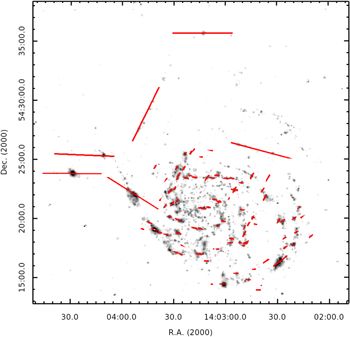
Figure 1. Map of H ii regions in NGC 5457 observed by this paper superimposed on an Hα image. Offsets in arcseconds, relative to the galaxy center, are given in Table 2. Short slits are part of multi-slit masks, whereas the long slits are single long-slit pointings.
Download figure:
Standard image High-resolution imageTable 1. Adopted Global Properties of NGC 5457
| Property | Adopted Value | Reference |
|---|---|---|
| R.A. | 14h03m12 5 5 |
(1) |
| Decl. | +54°20m56s | (1) |
| Inclination | 18° | (2) |
| Position Angle | 39° | (2) |
| Distance | 7.4 Mpc | (3) |
| R25 | 864'' | (4) |
Note. Units of R.A. are hours, minutes, and seconds, and units of decl. are degrees, arcminutes, and arcseconds.
References. References are as follows: (1) NED, (2) Walter et al. (2008), (3) Ferrarese et al. (2000), (4) Kennicutt et al. (2011).
Download table as: ASCIITypeset image
Our targeted regions (see Table 2), as well as alignment stars, were selected based on archival broadband and Hα imaging (Hoopes et al. 2001). We cut most slits to be ∼15'' long with a 1'' slit width. Slits were placed on relatively bright H ii regions across the entirety of the disk; this ensured that both radial and azimuthal trends in the abundances could be investigated. When extra space between slits was available, slits were extended to make the best use of the available field of view. As the bright disk of NGC 5457 complicates local sky subtraction, we also cut sky slits in each mask that provided a basis for clean sky subtraction.
For a detailed description of the data reduction procedures, we refer the reader to Berg et al. (2015). We only note here the primary points of our data processing. Spectra were reduced and analyzed using the development version of the MODS reduction pipeline6 which runs within the XIDL7 reduction package. One-dimensional (1D) spectra were corrected for atmospheric extinction and flux-calibrated based on observations of flux standard stars (Bohlin 2010). At least one flux standard was observed on each night science data were obtained. An example of a flux-calibrated spectrum is shown in Figure 2. Given that each light path traversed different physical portions of the dichroic, we extract a 1D flat spectrum for each object and subsequently correct the flux calibration of each spectrum individually using the ratio of the local flat spectrum and the flat spectrum extracted at the position of the standard star.
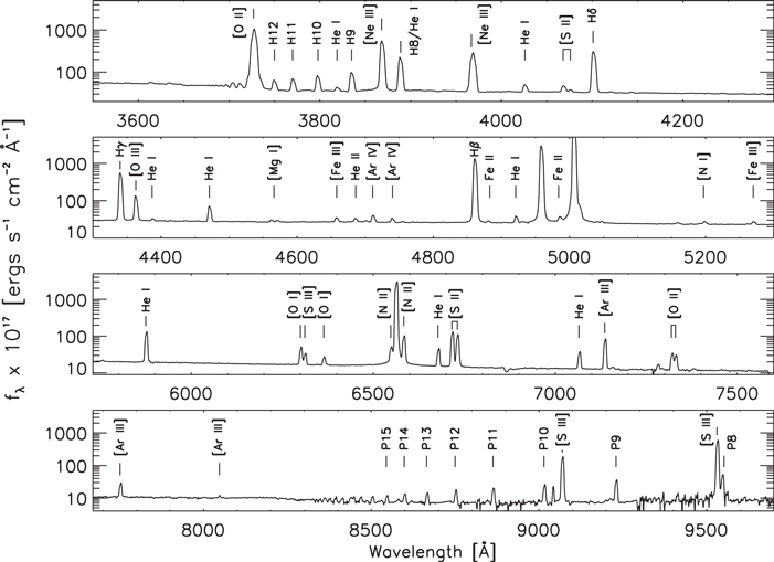
Figure 2. Example of a 1D spectrum taken from MODS1 observations of NGC 5457, namely NGC 5457+667.9+174.1. Notable major emission features are marked and labeled. We have not corrected for major telluric absorption features.
Download figure:
Standard image High-resolution imageWhile many H ii regions exist in the central region of NGC 5457, we chose to observe a few of these regions in multiple masks. This serves to confirm that our calibrations as stable and robust against changing observing conditions and permits us to obtain even deeper spectra in metal-rich regions near the center of NGC 5457 where the innate weakness of the auroral lines makes them difficult to detect. For regions with coverage in multiple slit masks, in general, we co-add individual flux-calibrated spectra to create the final spectrum. In two cases we did not co-add all the spectra as some were clearly more noisy. In all cases, analyses of the individual spectra are consistent with the summed spectrum.
2.2. Spectral Modeling and Line Intensities
We provide a detailed description of the adopted continuum modeling and line fitting procedures applied to the CHAOS observations in Berg et al. (2015). Here we will only highlight the principle components of the process. We model the underlying stellar continuum using the STARLIGHT8 spectral synthesis code (Cid Fernandes et al. 2005) in conjunction with the models of Bruzual & Charlot (2003). This allows us to fit for stellar absorption which is blended with the observed fine-structure lines.
Allowing for an additional faint nebular continuum, modeled as a linear component, we fit Gaussian profiles to each emission line. We note that blended emission lines in the Balmer sequence at the blue end of the spectrum (H7, H8, and H11–H14) are not fit but are modeled based on the measurements of unblended Balmer lines and the tabulated atomic ratios of Hummer & Storey (1987), assuming Case B recombination. As the line profiles are not perfect Gaussian's, we subsequently use the modeled baselines and positions to integrate under the continuum subtracted spectrum for all non-blended lines. In general, the difference between the flux returned by a Gaussian fit and direct integration is less than 2% of the line flux.
Given that precise measurements of the auroral lines are vital to this study, we measured the flux of each auroral line by hand in the extracted spectra to confirm the fit. While the majority of measurements were found to be in agreement, in cases where these measurements were in disagreement, we adopted the by hand measurement. This was most common for the [N ii] λ5755 line which falls in the wavelength region affected by the dichroic cutoff of MODS and the continuum here is not always well fit by the modeled starlight and the resultant fit was thus inadequate.
We correct the strength of emission features for line-of-sight reddening using the relative intensities of the three strongest Balmer lines (Hα/Hβ, Hα/Hγ, Hβ/Hγ). We report the determined values of c(Hβ) in Table 3. We do not apply an ad hoc correction to account for Balmer absorption as the lines were fit on top of stellar population models that accounted for this feature. We note that the stellar models contain stellar absorption with an equivalent width of ≈1–2 Å in the Hβ line. We report reddening-corrected line intensities measured from H ii regions in the target fields in Table 3.
The uncertainty associated with each measurement is determined from measurements of the spectral variance, extracted from the two-dimensional (2D) variance image, Poisson noise in the continuum, read noise, sky noise, flat fielding calibration error, error in continuum placement, and error in the determination of the reddening. We add, in quadrature, an additional 2% uncertainty based on the precision of the adopted flux calibration standards (Bohlin 2010, see discussion in Berg et al. 2015).
2.3. Diagnostic Diagrams
We targeted H ii regions using narrowband Hα imaging which was continuum subtracted. While Hα is prominent in the ionized gas of an H ii region, other objects besides H ii regions can also produce such emission. For example, planetary nebulae and supernovae remnants can be targeted based on the presence of ionized gas. To verify that we are measuring lines from photoionized H ii regions, we inspected standard diagnostic diagrams (Baldwin et al. 1981, BPT): [O iii]/Hβ versus [N ii]/Hα, [S ii]/Hα, and [O i]/Hα, and ionization parameter P versus R23, where


The standard BPT diagram, [O iii]/Hβ versus [N ii]/Hα, does not show any unusual regions. However, there are five regions, NGC 5457–250.8-52.0, NGC 5457+44.7+153.7, NGC 5457+650.1+270.7, NGC 5457+299.1+464.0, and NGC 5457–345.5+273.8, that stand out in both [S ii]/Hα and [O i]/Hα relative to [O iii]/Hβ. We have performed our analysis both including and excluding these data and found they alter neither the conclusions nor the fits to the abundance trends.
We also note that three regions NGC 5457–12.3–271.1, NGC 5457–219.4+308.7, and NGC 5457–167.8+321.5 lie offset from the trend of ionization parameter with R23 in the sense of a low-ionization parameter for the given R23. However, all other line diagnostics for these three regions are normal, and the spectra do not stand out as unusual. Therefore, we include these regions in our fits.
3. GAS-PHASE ABUNDANCES
The ability to determine an elemental abundance from an emission spectrum is dependent on knowledge of (1) the electron density (ne), (2) the electron temperature (Te), and (3) a correction factor for unobserved ionic states. Observationally, the challenge is to detect the intrinsically faint auroral lines, which, when paired with their stronger ionic counterparts, are sensitive to electron temperature (e.g., see Osterbrock & Ferland 2006). Lacking detections of these lines, one must turn to indirect methods, wherein measurements of the strong lines have been calibrated either empirically or via photoionization modeling (e.g., Edmunds & Pagel 1984). In calculating temperatures and abundances, we have adopted the updated atomic data presented in Berg et al. (2015).
3.1. Temperature Relations
We have measured electron temperatures using five ratios of auroral to nebular lines: [O iii] λ4363/λλ4959, 5007; [S iii] λ6312/λλ9069, 9532; [N ii] λ5755/λλ6548, 6583; [O ii] λλ7319, 7330/λλ3726, 3729; [S ii] λλ4069, 4076/λλ6717, 6731. The derived electron temperatures from the different ions are reported in Table 4. Different ions measure the electron temperature in physically different portions of an H ii region, depending on the energy needed to excite the relevant transitions, and thus present independent temperature scales. We have chosen to represent the temperature structure of an H ii region with a three-zone model. The different zones are characterized by different ionic temperatures. For the ionization stages represented in each zone, we adopt: [O ii], [N ii], [S ii] in the low-ionization zone; [S iii], [Ar iii] in the intermediate-ionization zone; and [O iii], [Ne iii] in the high-ionization zone.
One primary reason we selected NGC 5457 for this study was the large number of bright H ii regions that enhance the likelihood that multiple auroral lines will be detected in any given H ii region. Indeed, the ability to compare multiple temperature measures for a given H ii region allows us to compare the different temperature scales. Previous investigations of these relations has found very good agreement between the photoionization models of Garnett (1992), namely,


and the empirically measured temperatures from multiple ions (e.g., Kennicutt et al. 2003). In Croxall et al. (2015), we found good agreement between T[S iii] and T[N ii] in H ii regions in NGC 5194. However, no H ii regions in that sample have measurements of T[O iii] with which they may be compared. In Berg et al. (2015), we detected both the [O iii] and [S iii] auroral lines in several H ii regions. These showed an offset relative to Equation (3) and significant scatter, calling into question the rote acceptance of T[O iii] as ground truth. Following our practice in Berg et al. (2015), we adopt a theoretical ratio of λ9532/λ9069 = 2.51 to correct for possible contamination of the red end of the spectrum by atmospheric absorption.
The sensitivity of MODS on LBT allows us to greatly increase the number of regions used in a comparison of electron temperatures, even while restricting ourselves to a single galaxy, particularly when the selected galaxy has numerous luminous H ii regions, as is the case with NGC 5457. As noted in Berg et al. (2015), the current atomic data lead to significant changes in the temperatures derived from [S iii] and [O ii]. Given this change in atomic data since the Garnett (1992) models were run, changes in the resultant temperature relations would not be unreasonable.
We plot the various temperature–temperature relations in Figure 3. Linear regression fits are computed using the Bayesian method described by Kelly (2007) which accounts for measurement errors in both variables and includes explicit fitting for intrinsic scatter in the regression (see also Hogg et al. 2010 for a thorough discussion of this fitting problem in an astrophysical context). This method models the intrinsic scatter in the independent variables as a linear mixture of Gaussian distributions. We use J. Meyers' Python-language implementation of Kelly's original IDL code9 to perform the calculations. This implementation uses a Markov-Chain Monte Carlo to compute 10,000 samplings from the posteriors. We adopt as the "best-fit" parameters the medians of the resulting marginal posterior distributions for the slope, intercept, intrinsic scatter, and linear correlation coefficients, and evaluate the standard deviation of these posterior distributions to estimate the uncertainties for each fit parameter. We show the resulting fits as solid black lines; we also include Equations (3) and (4), the relations derived from the photoionization models of Garnett (1992), as dashed blue lines.
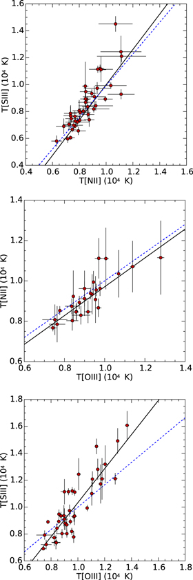
Figure 3. Relationship between T[N ii] and T[S iii] (top), T[O iii] and T[N ii] (middle), and T[O iii] and T[S iii] (bottom) measured for H ii regions in NGC 5457. The empirical relations from CHAOS observations as drawn as a solid black line while the photoionization models of Garnett (1992) are drawn as a dashed blue line. These temperature–temperature relations are characterized by intrinsic dispersions of 290 ± 60 K, 280 ± 140 K, and 1050 ± 160 K.
Download figure:
Standard image High-resolution imageAs can be seen in the top panel of Figure 3, we find a reasonable agreement with the models of Garnett (1992) when comparing T[N ii] and T[S iii]. We do measure a slight shift in both the slope and zero-point offset in the empirical relationship compared to the result of combining Equations (3) and (4). However, these differences are only at the one and two sigma level, respectively. Furthermore, in the region where data exist, the two relations show a striking similarity. These slight offsets are consistent with differences in atomic data we have adopted compared to the atomic data used by Garnett (1992).
In the middle panel of Figure 3, we show the relationship between T[N ii] and T[O iii]. In this case, we find agreement with the slope derived by Garnett (1992) and only note a slight shift in the zero-point offset of the relationship. While the zero-point offset is just over the three sigma confidence level, it can be explained given the differences in the adopted atomic data.
Similar to the results of Kennicutt et al. (2003), we find a good correlation between T[O iii] and T[S iii] in the 37 regions where both temperature-sensitive line ratios are measured, as shown in the bottom panel of Figure 3. However, in this case, we do not find good agreement with the models of Garnett (1992). Again, this may, in part, also arise from the different atomic data adopted; however, the atomic data alone cannot explain the difference. Rather, as shown in Figure 3, the empirical relationship between these two ionic temperatures is significantly steeper than that given by Equation (3). This is particularly important for cool H ii regions where the [S iii] auroral line is more frequently detected relative to the [O iii] auroral line. Indeed, in the coolest regions where the [S iii] λ6312 line is detected, the two different relations lead to temperatures that differ by more than 2,000 K. We also note that, in contrast with what was seen in NGC 628 (Berg et al. 2015), the relationship between T[O iii] and T[S iii] is fairly tight with a rms deviation of ≈2200 K, compared to the scatter we measure in the NGC 0628 data, ≈5000 K. Nevertheless, we do note that there are H ii regions which lie below this relation in the regime largely populated in NGC 628.
Two H ii regions, NGC 5457–397.4–71.7 and NGC 5457–226.9–366.4, exhibit anomalously high T[N ii] and have been excluded from these fits and plots. Kennicutt et al. (2003) also noted some discrepant points when comparing these two temperatures and concluded that unphysically high T[N ii] were likely the result of marginally detected lines. Careful investigation of our spectra do not support a similar conclusion for our two discrepant data points. Indeed, in the most discrepant of the two regions, NGC 5457–397.4–71.7, the [N ii] λ5755 line can be seen in each of the six individual 2D images, ensuring it is not an anomalous measurement due to contamination via cosmic rays. Rather, these anomalous temperatures likely indicate a complex environment in these giant star-forming complexes. The existence of such unusual temperature signatures can lead to highly skewed results if only a single-temperature measure is observed for a given H ii region.
Given that we derive abundances using different atomic data from those used in the models of Garnett (1992), applying those temperature relations would introduce systematic offsets. While previous data sets (e.g., Berg et al. 2015; Croxall et al. 2015) did not cover a large enough range of parameter space to truly constrain empirical temperature–temperature relations, the number of observed H ii regions with multiple temperature measurements and the steep oxygen gradient in NGC 5457 (Kennicutt et al. 2003) result in the ideal uniform data set to derive empirical temperature relations. We thus adopt the empirical temperature relations fit to CHAOS data for which multiple auroral lines were detected in a single region, namely:


and

These empirical relations are consistent with intrinsic dispersion of 280 ± 140 K, 290 ± 60 K, and 1050 ± 160 K, respectively. We adopt these values as lower limits for the uncertainty of a temperature derived via these relations. To ensure that we are not introducing additional bias in our abundance determinations by adopting these temperature relations, we confirm that offsets from Equations (5)–(7) do not correlate with the oxygen ion fraction, O+/O, or excitation.
In addition to measuring electron temperatures in each ionization zone of our three-zone model, we also measure three independent ionic ratios that characterize the low-ionization zone, T[O ii], T[S ii], and T[N ii]. The standard practice is to adopt either one of the temperature–temperature relations already discussed or to measure T[N ii]. This has arisen due to a large amount of scatter in T[O ii] and the relative weakness of the [S ii] auroral lines. The increased dispersion in T[O ii], compared to other measurements of electron temperature, has also been attributed to contributions from direct dielectric recombinations to the 2P0 level, from which the auroral lines arise (Rubin 1986). Furthermore, in the case of T[O ii] underlying telluric absorption, proximity of strong OH Meinel band emission, possible contribution due to recombination (Liu et al. 2000), and a susceptibility of [O ii] to collisional de-excitation complicate temperature measurements from [O ii] lines. Additionally the temperature-sensitive line ratios for [O ii] and [S ii] are separated by ≈3600 Å and ≈2600 Å, respectively, making them more sensitive to the effects of reddening.
Our measurements of T[O ii], T[S ii], and T[N ii] do indeed suggest that they largely arise from a common ionization zone. In Figure 4 we plot the T[O ii] against T[N ii] (top) and T[S ii] against T[N ii] (bottom) for those H ii regions where both respective sets of auroral lines were measured. While there is noticeable scatter about the one-to-one relation, with intrinsic dispersions of ≈900 K for T[S ii] and ≈1100 K for T[O ii], the three temperatures are clearly correlated and suggest that the three ions are roughly measuring the electron temperature in an equivalent volume of gas. While an exhaustive investigation of the [O ii] and [S ii] lines is not the purpose of this paper, we have looked for possible trends in the deviations of T[O ii] and T[S ii] from T[N ii]. We do not find any significant correlations with a variety of parameters such as the ionization parameters and reddening coefficient that might be expected given previous explanations of this scatter. Notably, restricting the sample to only the highest signal-to-noise detections does not decrease the scatter between these three temperatures.

Figure 4. Plots of T[O ii] against T[N ii] (top) and T[S ii] against T[N ii] (bottom) measured for H ii regions in NGC 5457. The dashed one-to-one line plotted shows that the data are in agreement with these ions being isothermal.
Download figure:
Standard image High-resolution image3.2. Comparison with Previous Work
Electron temperatures have previously been reported in a significant number of H ii regions in NGC 5457, making it a useful benchmark test for the CHAOS program. Notably, we have significant overlap with the samples of Kennicutt et al. (2003; 14/20 regions), Bresolin (2007; 2/2 regions), and Li et al. (2013; 6/10 regions). Given that we adopt slightly different atomic data (Berg et al. 2015), we take their reported line measurements and re-compute electron temperatures and abundances.
In Figure 5, we compare the derived electron temperatures from the line measurements reported in Kennicutt et al. (2003), Bresolin (2007), and Li et al. (2013) with those reported here. As can be seen, the calculated temperatures lie close to a one-to-one relation for all three ions used to independently derive the temperature. In warm regions, the [N ii] λ5755 line becomes more difficult to detect. This is reflected in the larger errors in the warmer H ii regions. Indeed, in two regions, NGC 5457–371.1–280.0 (H143) and NGC 5457–368.3–285.6 (H149), Kennicutt et al. (2003) adopt significantly lower temperatures for the low-ionization region based on temperatures derived from the [O iii] measurements. We do not plot these two regions in the right panel of Figure 5; however, we note that while their measured T[N ii] is highly discrepant from ours, their adopted value is in agreement with our measurements.
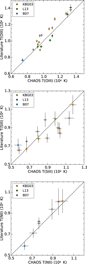
Figure 5. Comparison between temperatures derived from CHAOS spectra and those derived from the literature. A one-to-one correlation is plotted as a dashed gray line.
Download figure:
Standard image High-resolution imageIn addition to electron temperatures, we report line strengths and the recomputed oxygen, nitrogen, and sulfur abundances for H ii regions measured in the literature and our newly obtained data in Table 5. In general, we find very good agreement between the abundances derived from reported line strengths in Kennicutt et al. (2003), Bresolin (2007), and Li et al. (2013) and those presented in this work, with an average difference in 12 + log(O/H) and log(N/O) of 0.02 dex and 0.08, respectively.
Table 2. NGC 5457 MODS/LBT Observations
| H ii | R.A. | Decl. | P.A. | Extraction |

|
Auroral Line Detections | Alt. | ||||||
|---|---|---|---|---|---|---|---|---|---|---|---|---|---|
| Region | (2000) | (2000) | (arcsec) | [O iii] | [N ii] | [S iii] | [O ii] | [S ii] | WR | He ii | Name | ||
| Total Detections: | 50 | 47 | 59 | 67 | 70 | 30 | 10 | ||||||
| +7.2-3.8 | 14:03:13.3 | 54:20:52.16 | 85 | 4 | 0.010 | ⋯ | ⋯ | ⋯ | ⋯ | ⋯ | ⋯ | ⋯ | H678 |
| −22.0+1.6 | 14:03:10.0 | 54:20:57.55 | 80 | 8 | 0.027 | ⋯ | ✓ | ⋯ | ⋯ | ⋯ | ⋯ | ⋯ | H602 |
| −52.1+41.2 | 14:03:06.5 | 54:21:37.23 | 80 | 7 | 0.081 | ⋯ | ⋯ | ⋯ | ⋯ | ⋯ | ⋯ | ⋯ | H555 |
| −75.0+29.3 | 14:03:03.9 | 54:21:25.29 | 80 | 6.5 | 0.098 | ⋯ | ✓ | ✓ | ⋯ | ⋯ | ✓ | ⋯ | H493 |
| +22.1-102.1 | 14:03:15.0 | 54:19:13.93 | 70 | 5 | 0.125 | ⋯ | ✓ | ⋯ | ⋯ | ✓ | ⋯ | ⋯ | H699 |
| +20.0-104.4 | 14:03:14.8 | 54:19:11.63 | 70 | 8 | 0.127 | ⋯ | ⋯ | ⋯ | ⋯ | ✓ | ⋯ | ⋯ | H686 |
| −70.6-92.8 | 14:03:04.4 | 54:19:23.17 | 80 | 8 | 0.135 | ⋯ | ⋯ | ⋯ | ⋯ | ✓ | ✓ | ⋯ | H505 |
| +47.9-103.2 | 14:03:18.0 | 54:19:12.82 | 80 | 8 | 0.137 | ⋯ | ✓ | ⋯ | ⋯ | ✓ | ⋯ | ⋯ | H760 |
| −96.2-68.7 | 14:03:01.5 | 54:19:47.23 | 80 | 6 | 0.138 | ⋯ | ⋯ | ⋯ | ⋯ | ⋯ | ⋯ | ⋯ | H451 |
| −12.0+139.0 | 14:03:11.1 | 54:23:15.01 | 145 | 7 | 0.165 | ⋯ | ✓ | ⋯ | ✓ | ✓ | ⋯ | ⋯ | H620 |
| +138.9+30.6 | 14:03:28.4 | 54:21:26.49 | 145 | 8 | 0.167 | ⋯ | ✓ | ✓ | ✓ | ✓ | ✓ | ⋯ | H972 |
| +134.4-58.8 | 14:03:27.9 | 54:19:57.11 | 70 | 7 | 0.178 | ⋯ | ✓ | ✓ | ✓ | ✓ | ⋯ | ⋯ | H959 |
| +44.7+153.7 | 14:03:17.6 | 54:23:29.66 | 85 | 4 | 0.186 | ⋯ | ⋯ | ⋯ | ⋯ | ✓ | ⋯ | ⋯ | H768 |
| −44.1+149.5 | 14:03:07.4 | 54:23:25.50 | 85 | 6 | 0.187 | ⋯ | ⋯ | ⋯ | ⋯ | ⋯ | ⋯ | ⋯ | H567 |
| +164.6+9.9 | 14:03:31.3 | 54:21:05.81 | 145 | 10 | 0.196 | ✓ | ✓ | ✓ | ✓ | ✓ | ✓ | ⋯ | H1013 |
| +89.3+149.7 | 14:03:22.7 | 54:23:25.66 | 85 | 5 | 0.202 | ⋯ | ✓ | ✓ | ⋯ | ✓ | ⋯ | ⋯ | H864 |
| +68.2+161.8 | 14:03:20.3 | 54:23:37.77 | 85 | 4 | 0.204 | ⋯ | ⋯ | ⋯ | ⋯ | ✓ | ⋯ | ⋯ | H813 |
| +149.8+92.4 | 14:03:29.6 | 54:22:28.31 | 145 | 3 | 0.204 | ⋯ | ⋯ | ⋯ | ✓ | ✓ | ⋯ | ⋯ | H998 |
| −70.2+162.2 | 14:03:04.5 | 54:23:38.19 | 85 | 4 | 0.213 | ⋯ | ✓ | ✓ | ✓ | ✓ | ⋯ | ⋯ | H504 |
| +166.4+86.3 | 14:03:31.5 | 54:22:22.20 | 145 | 7.5 | 0.218 | ⋯ | ✓ | ✓ | ✓ | ✓ | ✓ | ⋯ | H1018 |
| +177.2-42.8 | 14:03:32.8 | 54:20:13.07 | 70 | 6 | 0.220 | ⋯ | ✓ | ✓ | ✓ | ✓ | ✓ | ⋯ | H1045 |
| −159.9+89.6 | 14:02:54.2 | 54:22:25.56 | 85 | 8 | 0.223 | ⋯ | ✓ | ✓ | ✓ | ✓ | ✓ | ⋯ | H336 |
| +133.1-126.8 | 14:03:27.7 | 54:18:49.17 | 70 | 5 | 0.223 | ⋯ | ✓ | ✓ | ✓ | ✓ | ✓ | ⋯ | H949 |
| +177.2+76.1 | 14:03:32.8 | 54:22:12.03 | 145 | 6 | 0.225 | ⋯ | ✓ | ✓ | ✓ | ✓ | ✓ | ⋯ | H1040 |
| −190.6-10.8 | 14:02:50.7 | 54:20:45.05 | 80 | 5 | 0.228 | ⋯ | ⋯ | ⋯ | ⋯ | ⋯ | ⋯ | ⋯ | H280 |
| +134.8+146.0 | 14:03:27.9 | 54:23:21.97 | 145 | 2 | 0.230 | ⋯ | ⋯ | ⋯ | ⋯ | ⋯ | ⋯ | ⋯ | H967 |
| −120.2+146.9 | 14:02:58.7 | 54:23:22.84 | 85 | 5 | 0.231 | ⋯ | ✓ | ✓ | ✓ | ✓ | ✓ | ⋯ | H399 |
| −123.1+146.1 | 14:02:58.4 | 54:23:22.09 | 85 | 4 | 0.232 | ⋯ | ⋯ | ⋯ | ⋯ | ⋯ | ⋯ | ⋯ | H387 |
| +130.2+157.4 | 14:03:27.4 | 54:23:33.39 | 145 | 7 | 0.236 | ⋯ | ✓ | ✓ | ✓ | ✓ | ✓ | ⋯ | H953 |
| +200.3-0.4 | 14:03:35.4 | 54:20:55.42 | 145 | 6.25 | 0.239 | ⋯ | ⋯ | ⋯ | ✓ | ⋯ | ✓ | ⋯ | H1071 |
| +129.2+161.7 | 14:03:27.3 | 54:23:37.62 | 145 | 2 | 0.239 | ⋯ | ⋯ | ✓ | ✓ | ✓ | ⋯ | ⋯ | H941 |
| −139.7-157.6 | 14:02:56.5 | 54:18:18.31 | 80 | 10 | 0.244 | ⋯ | ⋯ | ⋯ | ⋯ | ✓ | ⋯ | ✓ | H355, NGC 5453 |
| −145.1+146.8 | 14:02:55.9 | 54:23:22.72 | 85 | 4 | 0.251 | ⋯ | ⋯ | ✓ | ✓ | ✓ | ⋯ | ⋯ | H351 |
| +103.5+192.6 | 14:03:24.4 | 54:24:08.61 | 145 | 5 | 0.253 | ⋯ | ✓ | ✓ | ✓ | ✓ | ⋯ | ⋯ | H888 |
| −66.9-210.8 | 14:03:04.9 | 54:17:25.19 | 90 | 3.5 | 0.258 | ⋯ | ⋯ | ⋯ | ⋯ | ⋯ | ⋯ | ⋯ | H510 |
| −133.9-178.7 | 14:02:57.2 | 54:17:57.24 | 90 | 4 | 0.259 | ⋯ | ⋯ | ⋯ | ⋯ | ⋯ | ✓ | ⋯ | H363, NGC 5453 |
| −205.4-98.2 | 14:02:49.0 | 54:19:17.63 | 150 | 4 | 0.267 | ⋯ | ✓ | ✓ | ✓ | ✓ | ✓ | ⋯ | H246 |
| −192.5+124.7 | 14:02:50.5 | 54:23:00.57 | 85 | 10 | 0.279 | ⋯ | ⋯ | ⋯ | ⋯ | ⋯ | ⋯ | ⋯ | H284 |
| +17.3-235.4 | 14:03:14.5 | 54:17:00.55 | 90 | 8 | 0.280 | ✓ | ✓ | ✓ | ✓ | ✓ | ⋯ | ⋯ | H694, NGC 5458 |
| +36.8-233.4 | 14:03:16.7 | 54:17:02.61 | 70 | 6 | 0.281 | ⋯ | ✓ | ✓ | ✓ | ✓ | ⋯ | ⋯ | H728, NGC 5458 |
| −226.8-77.8 | 14:02:46.6 | 54:19:38.00 | 150 | 12 | 0.282 | ⋯ | ⋯ | ⋯ | ⋯ | ⋯ | ⋯ | ⋯ | H223 |
| +139.0+200.7 | 14:03:28.4 | 54:24:16.62 | 145 | 7 | 0.282 | ⋯ | ✓ | ⋯ | ✓ | ✓ | ⋯ | ⋯ | H969 |
| −205.2-128.7 | 14:02:49.1 | 54:18:47.16 | 150 | 3 | 0.282 | ⋯ | ⋯ | ⋯ | ⋯ | ⋯ | ⋯ | ⋯ | H255 |
| +189.2-136.3 | 14:03:34.1 | 54:18:39.60 | 70 | 4 | 0.284 | ✓ | ✓ | ✓ | ✓ | ✓ | ✓ | ⋯ | H1052 |
| −203.8-135.6 | 14:02:49.2 | 54:18:40.30 | 150 | 4 | 0.285 | ⋯ | ⋯ | ⋯ | ⋯ | ⋯ | ⋯ | ⋯ | H247 |
| −183.9-179.0 | 14:02:51.5 | 54:17:56.90 | 80 | 9 | 0.298 | ✓ | ✓ | ✓ | ✓ | ✓ | ⋯ | ⋯ | H290 |
| −249.4-51.3 | 14:02:44.0 | 54:20:04.54 | 80 | 9 | 0.301 | ⋯ | ⋯ | ✓ | ✓ | ✓ | ⋯ | ⋯ | H203 |
| −250.8-52.0 | 14:02:43.8 | 54:20:03.81 | 80 | 3.5 | 0.303 | ⋯ | ⋯ | ✓ | ✓ | ✓ | ⋯ | ✓ | H203 |
| +225.6-124.1 | 14:03:38.3 | 54:18:51.72 | 70 | 7 | 0.313 | ✓ | ✓ | ✓ | ✓ | ✓ | ⋯ | ⋯ | H1086, NGC 5461 |
| +117.9-235.0 | 14:03:26.0 | 54:17:00.95 | 70 | 7 | 0.317 | ✓ | ⋯ | ✓ | ✓ | ✓ | ⋯ | ✓ | H922 |
| −208.0-180.7 | 14:02:48.7 | 54:17:55.12 | 80 | 10 | 0.320 | ✓ | ✓ | ✓ | ✓ | ✓ | ⋯ | ⋯ | H237 |
| −12.3-271.1 | 14:03:11.1 | 54:16:24.95 | 90 | 4 | 0.320 | ⋯ | ✓ | ✓ | ✓ | ✓ | ✓ | ⋯ | H618 |
| +142.8-225.2 | 14:03:28.8 | 54:17:10.76 | 70 | 4 | 0.323 | ⋯ | ⋯ | ⋯ | ✓ | ✓ | ⋯ | ✓ | H971 |
| −200.3-193.6 | 14:02:49.6 | 54:17:42.25 | 90 | 16 | 0.323 | ✓ | ⋯ | ✓ | ✓ | ✓ | ✓ | ⋯ | H260 |
| +96.7+266.9 | 14:03:23.6 | 54:25:22.90 | 145 | 8 | 0.330 | ✓ | ✓ | ✓ | ✓ | ✓ | ✓ | ⋯ | H875 |
| +67.5+277.0 | 14:03:20.2 | 54:25:33.00 | 145 | 4 | 0.333 | ✓ | ✓ | ✓ | ✓ | ✓ | ⋯ | ⋯ | H798 |
| +252.2-109.8 | 14:03:41.3 | 54:19:05.96 | 70 | 4 | 0.333 | ✓ | ✓ | ✓ | ✓ | ✓ | ⋯ | ✓ | H1100, NGC 5461 |
| +254.6-107.2 | 14:03:41.6 | 54:19:08.55 | 70 | 9 | 0.335 | ✓ | ✓ | ✓ | ✓ | ✓ | ✓ | ⋯ | H1105, NGC 5461 |
| +281.4-71.8 | 14:03:44.7 | 54:19:43.98 | 70 | 8 | 0.350 | ✓ | ⋯ | ✓ | ✓ | ✓ | ⋯ | ✓ | H1122 |
| −243.0+159.6 | 14:02:44.7 | 54:23:35.38 | 150 | 4 | 0.354 | ✓ | ✓ | ✓ | ✓ | ✓ | ⋯ | ⋯ | H206 |
| +249.3+201.9 | 14:03:41.1 | 54:24:17.71 | 145 | 5 | 0.372 | ✓ | ✓ | ✓ | ✓ | ✓ | ⋯ | ⋯ | H1104 |
| −297.7+87.1 | 14:02:38.4 | 54:22:22.84 | 150 | 6 | 0.375 | ✓ | ✓ | ✓ | ✓ | ✓ | ⋯ | ⋯ | H185 |
| −309.4+56.9 | 14:02:37.1 | 54:21:52.56 | 150 | 13 | 0.379 | ✓ | ⋯ | ⋯ | ✓ | ⋯ | ⋯ | ⋯ | H181, NGC 5451 |
| +354.1+71.2 | 14:03:53.0 | 54:22:06.80 | 60 | 7 | 0.426 | ✓ | ✓ | ✓ | ✓ | ✓ | ⋯ | ⋯ | H1170, NGC 5462 |
| −164.9-333.9 | 14:02:53.7 | 54:15:22.03 | 90 | 6 | 0.433 | ✓ | ✓ | ✓ | ✓ | ✓ | ✓ | ⋯ | H321 |
| +360.9+75.3 | 14:03:53.8 | 54:22:10.81 | 60 | 8 | 0.435 | ✓ | ⋯ | ✓ | ✓ | ✓ | ⋯ | ⋯ | H1174, NGC 5462 |
| −167.8+321.5 | 14:02:53.3 | 54:26:17.43 | 75 | 6 | 0.438 | ⋯ | ⋯ | ⋯ | ⋯ | ⋯ | ⋯ | ⋯ | H295 |
| −178.0+319.1 | 14:02:52.1 | 54:26:14.95 | 75 | 16 | 0.442 | ⋯ | ⋯ | ✓ | ✓ | ✓ | ✓ | ⋯ | H317 |
| −377.9-64.9 | 14:02:29.3 | 54:19:50.65 | 150 | 13 | 0.454 | ✓ | ✓ | ✓ | ✓ | ✓ | ⋯ | ⋯ | H140, NGC 5449 |
| −209.1+311.8 | 14:02:48.5 | 54:26:07.69 | 75 | 8 | 0.455 | ⋯ | ⋯ | ⋯ | ⋯ | ⋯ | ✓ | ⋯ | ⋯ |
| −219.4+308.7 | 14:02:47.4 | 54:26:04.51 | 75 | 4.5 | 0.459 | ⋯ | ⋯ | ⋯ | ⋯ | ⋯ | ⋯ | ⋯ | ⋯ |
| −225.0+306.6 | 14:02:46.7 | 54:26:02.45 | 75 | 4 | 0.461 | ⋯ | ⋯ | ⋯ | ⋯ | ⋯ | ⋯ | ⋯ | H234 |
| −99.6-388.0 | 14:03:01.1 | 54:14:27.97 | 90 | 5 | 0.468 | ✓ | ✓ | ✓ | ✓ | ✓ | ✓ | ⋯ | H416, NGC 5455 |
| −397.4-71.7 | 14:02:27.1 | 54:19:43.76 | 124 | 11 | 0.478 | ✓ | ✓ | ⋯ | ⋯ | ⋯ | ⋯ | ⋯ | H115, NGC 5449 |
| −222.9-366.4 | 14:02:47.1 | 54:14:49.40 | 90 | 2 | 0.497 | ⋯ | ⋯ | ⋯ | ⋯ | ✓ | ⋯ | ⋯ | H231 |
| −226.9-366.4 | 14:02:46.6 | 54:14:49.40 | 90 | 7 | 0.500 | ✓ | ✓ | ✓ | ✓ | ✓ | ⋯ | ⋯ | H219 |
| −405.5-157.7 | 14:02:26.2 | 54:18:17.79 | 124 | 10 | 0.511 | ✓ | ⋯ | ⋯ | ✓ | ✓ | ✓ | ⋯ | H104 |
| −345.5+273.8 | 14:02:32.9 | 54:25:29.41 | 75 | 3 | 0.537 | ✓ | ⋯ | ✓ | ✓ | ✓ | ⋯ | ⋯ | H167 |
| −410.3-206.3 | 14:02:25.6 | 54:17:29.09 | 124 | 4 | 0.537 | ✓ | ✓ | ✓ | ✓ | ✓ | ✓ | ⋯ | H103 |
| −371.1-280.0 | 14:02:30.1 | 54:16:15.53 | 124 | 8 | 0.540 | ✓ | ✓ | ✓ | ✓ | ✓ | ✓ | ⋯ | H143, NGC 5447 |
| −368.3-285.6 | 14:02:30.5 | 54:16:09.89 | 124 | 9 | 0.541 | ✓ | ✓ | ✓ | ✓ | ✓ | ✓ | ⋯ | H149, NGC 5447 |
| −455.7-55.8 | 14:02:20.4 | 54:19:59.55 | 124 | 17 | 0.545 | ✓ | ⋯ | ✓ | ✓ | ✓ | ⋯ | ⋯ | H59 |
| −392.0-270.1 | 14:02:27.8 | 54:16:25.34 | 124 | 13 | 0.554 | ✓ | ✓ | ✓ | ✓ | ✓ | ✓ | ⋯ | H128, NGC 5447 |
| −414.1-253.6 | 14:02:25.2 | 54:16:41.84 | 124 | 4 | 0.566 | ✓ | ✓ | ✓ | ✓ | ✓ | ⋯ | ⋯ | H98 |
| −464.7-131.0 | 14:02:19.4 | 54:18:44.25 | 124 | 4 | 0.569 | ✓ | ⋯ | ✓ | ✓ | ✓ | ⋯ | ⋯ | H51 |
| −466.1-128.2 | 14:02:19.2 | 54:18:47.06 | 124 | 4 | 0.570 | ✓ | ⋯ | ✓ | ✓ | ✓ | ⋯ | ⋯ | H46 |
| −479.7-3.9 | 14:02:17.6 | 54:20:51.33 | 124 | 4 | 0.573 | ✓ | ⋯ | ✓ | ✓ | ⋯ | ⋯ | ⋯ | H35 |
| −481.4-0.5 | 14:02:17.4 | 54:20:54.75 | 124 | 4 | 0.575 | ✓ | ⋯ | ✓ | ✓ | ✓ | ✓ | ⋯ | H27 |
| −453.8-191.8 | 14:02:20.7 | 54:17:43.47 | 124 | 14 | 0.577 | ✓ | ✓ | ✓ | ✓ | ✓ | ⋯ | ⋯ | H71 |
| +331.9+401.0 | 14:03:50.6 | 54:27:36.60 | 153.7 | 8 | 0.602 | ✓ | ⋯ | ⋯ | ✓ | ⋯ | ⋯ | ⋯ | H1151 |
| +324.5+415.8 | 14:03:49.7 | 54:27:51.46 | 153.7 | 9 | 0.610 | ✓ | ⋯ | ⋯ | ⋯ | ⋯ | ⋯ | ⋯ | H1148 |
| +315.3+434.4 | 14:03:48.7 | 54:28:10.10 | 153.7 | 4 | 0.621 | ✓ | ⋯ | ⋯ | ⋯ | ⋯ | ⋯ | ⋯ | H1146 |
| +299.1+464.0 | 14:03:46.8 | 54:28:39.70 | 153.7 | 5 | 0.639 | ⋯ | ⋯ | ⋯ | ⋯ | ⋯ | ⋯ | ⋯ | H1137 |
| −540.5-149.9 | 14:02:10.7 | 54:18:25.13 | 124 | 9 | 0.661 | ✓ | ⋯ | ✓ | ✓ | ✓ | ⋯ | ⋯ | H8 |
| +509.5+264.1 | 14:04:10.9 | 54:25:19.20 | 87.5 | 16 | 0.669 | ✓ | ✓ | ✓ | ✓ | ✓ | ⋯ | ✓ | H1216 |
| +266.0+534.1 | 14:03:43.0 | 54:29:49.89 | 153.7 | 8 | 0.692 | ✓ | ⋯ | ⋯ | ✓ | ⋯ | ✓ | ⋯ | H1125 |
| +667.9+174.1 | 14:04:29.0 | 54:23:48.56 | 90 | 4 | 0.813 | ✓ | ✓ | ✓ | ✓ | ✓ | ✓ | H1239, NGC 5471 | |
| +650.1+270.7 | 14:04:27.0 | 54:25:25.29 | 87.5 | 5 | 0.824 | ✓ | ⋯ | ⋯ | ⋯ | ⋯ | ⋯ | ✓ | H1231 |
| +692.1+272.9 | 14:04:31.8 | 54:25:27.24 | 87.5 | 4 | 0.871 | ✓ | ⋯ | ✓ | ✓ | ⋯ | ⋯ | ⋯ | H1248 |
| +1.0+885.8 | 14:03:12.6 | 54:35:41.83 | 90 | 4 | 1.046 | ✓ | ⋯ | ⋯ | ⋯ | ⋯ | ⋯ | ✓ | H681 |
| +6.6+886.3 | 14:03:13.3 | 54:35:42.29 | 90 | 21 | 1.046 | ✓ | ⋯ | ⋯ | ✓ | ⋯ | ⋯ | ⋯ | H641 |
| −8.5+886.7 | 14:03:11.5 | 54:35:42.70 | 90 | 8 | 1.048 | ✓ | ⋯ | ⋯ | ⋯ | ⋯ | ⋯ | ⋯ | H672 |
Note. Observing logs for H ii regions observed in NGC 5457 using MODS on the LBT during the 2015A semester. Each exposure was taken with an integrated exposure time of 1200 s on clear nights, with, on average, ∼100 seeing, and airmasses less than 1.3. Slit ID, composed of the offset in R.A. and decl., in arcseconds, from the central position listed in Table 1 is listed in Column 1. The R.A. and decl. of the individual H ii regions are given in units of hours, minutes, and seconds, and degrees, arcminutes, and arcseconds respectively in Columns 2 and 3. We list the position angle of the slit and the size of the region extracted along each slit in Columns 4 and 5. The de-projected distances of H ii regions from the center of the galaxy as a fraction of R25 is listed in Column 6. Columns 7–11 highlight which regions have [O iii] λ4363, [N ii] λ5755, [S iii] λ6312, [O ii] 7330, [S ii] λ4070 auroral lines detections at the 3σ significance level. We note in columns 12 and 13 which H ii regions have detections of broad Wolf–Rayet features and narrow He ii λ4686 emission. Finally Column 14 reports alternate names for the observed H ii regions primarily taken from Hodge et al. (1990).
Only a portion of this table is shown here to demonstrate its form and content. A machine-readable version of the full table is available.
While most H ii regions we have in common with previous reported studies are in agreement within the stated errors, two regions exhibit significant deviations. Comparing abundance determinations in NGC 5457+354.1+71.2 and NGC 5457–75.0+29.3 reveals that our new line measurements yield gas-phase oxygen abundances that are discrepant at the level of 0.25 dex, well above the stated errors, compared to recomputed abundances. However, the recomputed abundances are also not in agreement with the original computed abundances. In the case of NGC 5457+354.1+71.2, Kennicutt et al. (2003) do not adopt the temperature derived from the [O iii] λ4363 line. Rather, they adopt a significantly lower temperature for this H ii region, which places it in agreement with our CHAOS observations. On the other hand, the individual electron temperatures derived for NGC 5457–75.0+29.3 are all in agreement, while specific ionic abundances seem to be highly discrepant. The large differences for the recomputed abundances in these two regions could easily be due to typographical errors in the published tables of line strengths, so we compare our CHAOS data with the published abundances from the original works.
3.3. Electron Densities and Temperature Selections
To calculate abundances in regions where one or more temperature-sensitive line ratios were measured, we adopt an electron density, ne, based on the [S ii] λ6717/6731 line ratio as these relatively strong lines are cleanly separated in MODS1 spectra. The large majority of H ii regions observed, 95 out of 109, lie in the low-density regime [I(λ6717)/I(λ6731) > 1.35]. For these regions, we thus adopt an ne of 100 cm−3. For the remaining 14 regions, we calculate electron densities using a 5-level atom code based on FIVEL (De Robertis et al. 1987); see Table 4. Although these regions have densities that are higher than the low-density limit, they are all still low enough that collisional de-excitation is not an important factor. We note that the [O ii] λλ3726, 3729 doublet is blended for all observations; however, in the majority of spectra, the doublet profile is clearly non-Gaussian. We have modeled this doublet using two Gaussian profiles for use primarily as a consistency check of the [S ii] density determination. For all calculations aside from this density check, we sum the flux in the [O ii] λλ3726, 3729 doublet.
In regions where we have measured T[O iii], T[S iii], and T [N ii], we adopt the measured temperatures for each individual ionization zone when calculating abundances. When one or more of these temperatures have not been measured, we use Equations (5)–(7) to calculate a temperature for the ionization zone that is not measured. Given the scatter measured in the new temperature–temperature relations, where possible, T[N ii] is selected over T[S iii] where estimating T [O iii]; similarly, T[O iii] is preferentially selected to estimate T [N ii]. When an ionic temperature is calculated via Equations (5)–(7), the intrinsic dispersion for the relation used is adopted as the uncertainty in that adopted temperature. Both measured temperatures and the adopted temperatures are reported in Table 4.
3.4. Ionization Correction Factors (ICFs)
Nebular oxygen abundances obtained from optical spectra are quite straightforward. Given the similar ionization potentials of neutral hydrogen and oxygen, 13.60 eV and 13.62 eV, respectively, we can reasonably assume that all the oxygen in an H ii region is ionized. Furthermore, the high-ionization potential of O++, 54.94 eV, means that O+++ is also negligible in typical H ii regions. Thus, we can account for all oxygen ions present by summing the number of singly and doubly ionized oxygen ions. Unfortunately, other elements do not have a correspondingly simple pairing of observable lines in all ionization species and we must account for the presence of unobserved ionization states.
While many studies have investigated ICFs, most empirical studies are focused on higher ionization nebulae where auroral lines are easier to detect. By expanding our study toward low-ionization H ii regions, we must explore different options in ICFs and the regime in which each correction is valid. We refer the interested reader to the
To derive nitrogen abundances, we assume N/O = N+/O+, given the well matched ionization potential of these two species. Neon abundances were derived under the assumption Ne/O = Ne++/O++ (Peimbert & Costero 1969). The ICF for sulfur becomes more challenging in low-ionization nebulae as the parameter space has not been fully explored empirically. Thus, we adopt

for O+/O ≥ 0.4 and the ionization correction of Thuan et al. (1995) for O+/O ≤ 0.4. Similar to Kennicutt et al. (2003), we find the ratio of Ar++/S++ traces the Ar/S ratio. However, for low-ionization nebulae we adopt a linear correction to Ar++/S++,

to account for an increase in the Ar+ population. We report all ICFs and abundance ratios in Table 4.
3.5. Abundance Gradients
We calculate the de-projected distance from the galaxy center in units of the isophotal radius, R25, using the parameters given in Table 1. We plot the radial abundance gradients for O/H, N/O, S/O, Ar/O, and Ne/O in Figure 6. The CHAOS observations span the disk of NGC 5457 from R/R25 ∼ 0.10 to R/R25 ∼ 1.05, and including previously published direct abundances extends that outward to R/R25 ∼ 1.25. For consistency, we have, in addition to recomputing the abundances using new atomic data as described above, de-projected the distance to each H ii region using the same parameters. When a given H ii region is present in multiple samples, we have elected to adopt the new measurements from this study.
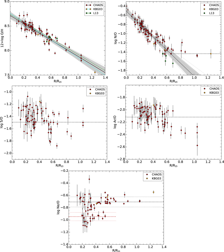
Figure 6. Radial abundance gradients in NGC 5457. Points are color-coded by study of origin. We have recomputed all abundances using identical atomic data and temperature–temperature relations. We plot the O/H and N/O abundance gradients we derive from direct abundance determinations as solid lines, with the flattened portion of the N/O gradient plotted as a dashed line. We include data from H ii regions in which auroral lines are not detected as smaller points on the N/O gradient, as this quantity is relatively insensitive to the electron temperature. For the S/O and Ar/O gradients we plot the weighted-mean value of the data as a dashed line. For Ne/O the dashed line indicates the mean of data with a log(Ne/O) greater than −0.9.
Download figure:
Standard image High-resolution imageWe note that the N/O abundance ratio is insensitive to changes in temperature because the temperature sensitivities of N+ and O+ are very similar. Thus, in regions where we do not any detect auroral line, we report the assumed temperature and derived N/O values in Table 6. These are based on a semi-empirical approach (van Zee et al. 1997), where an electron temperature is used to calculate the relative N/O abundance ratio. Specifically, we use an electron temperature consistent with the average of the the R-calibration and the S-calibration from Pilyugin & Grebel (2016).
Table 3. Line Fluxes Relative to Hβ
| Ion | NGC 5457+7.2–3.8 | NGC 5457–22.0+1.6 | NGC 5457–52.1+41.2 | NGC 5457–75.0+29.3 | NGC 5457+22.1–102.1 |
|---|---|---|---|---|---|
| [O ii] λ3726 | 0.1890 ± 0.0092 | 0.2130 ± 0.0053 | 0.430 ± 0.016 | 0.320 ± 0.010 | 0.500 ± 0.013 |
| [O ii] λ3729 | 0.450 ± 0.017 | 0.2310 ± 0.0056 | 0.380 ± 0.019 | 0.430 ± 0.012 | 0.880 ± 0.021 |
| H13 λ3734 | 0.0308 ± 0.0040 | 0.0240 ± 0.0010 | 0.0226 ± 0.0041 | 0.01950 ± 0.00075 | 0.0194 ± 0.0010 |
| H12 λ3750 | 0.0266 ± 0.0049 | 0.0378 ± 0.0024 | 0.0490 ± 0.0069 | 0.0267 ± 0.0013 | 0.0172 ± 0.0047 |
| H11 λ3771 | 0.0689 ± 0.0029 | 0.0382 ± 0.0029 | 0.0415 ± 0.0057 | 0.0417 ± 0.0022 | 0.0293 ± 0.0027 |
| H10 λ3798 | 0.0658 ± 0.0085 | 0.0522 ± 0.0022 | 0.0491 ± 0.0089 | 0.0424 ± 0.0016 | 0.0422 ± 0.0022 |
| He i λ3820 | ≤0.180 | ≤0.051 | ≤0.150 | 0.0060 ± 0.0010 | 0.0094 ± 0.0027 |
| H9 λ3835 | 0.0824 ± 0.0045 | 0.0624 ± 0.0018 | 0.0568 ± 0.0046 | 0.0655 ± 0.0023 | 0.0713 ± 0.0028 |
| [Ne iii] λ3869 | ≤0.0198 | ≤0.0103 | ≤0.160 | ≤0.00242 | 0.0133 ± 0.0022 |
| He i λ3889 | 0.0639 ± 0.0060 | 0.0328 ± 0.0029 | 0.0232 ± 0.0073 | 0.0423 ± 0.0029 | 0.0553 ± 0.0027 |
| H8 λ3889 | 0.120 ± 0.016 | 0.1010 ± 0.0043 | 0.095 ± 0.017 | 0.0824 ± 0.0030 | 0.0819 ± 0.0042 |
| He i λ3965 | ≤0.053 | ≤0.062 | ≤0.120 | ≤0.070 | ≤0.053 |
| [Ne iii] λ3967 | ≤0.047 | ≤0.072 | ≤0.140 | 0.0280 ± 0.0033 | 0.0477 ± 0.0024 |
| H7 λ3970 | 0.180 ± 0.024 | 0.1510 ± 0.0063 | 0.140 ± 0.026 | 0.1230 ± 0.0044 | 0.1220 ± 0.0063 |
| Fe i λ4010 | ≤0.160 | 0.0112 ± 0.0027 | ≤0.092 | 0.0036 ± 0.0012 | ≤0.054 |
| He i λ4026 | ≤0.230 | 0.0095 ± 0.0011 | ≤0.130 | 0.0071 ± 0.0017 | ≤0.054 |
| [S ii] λ4069 | ≤0.046 | ≤0.0091 | ≤0.050 | 0.0054 ± 0.0014 | ≤0.0281 |
| [S ii] λ4076 | ≤0.094 | 0.0075 ± 0.0016 | ≤0.049 | ≤0.0048 | ≤0.0293 |
| Hdelta λ4102 | 0.2280 ± 0.0057 | 0.2400 ± 0.0055 | 0.2310 ± 0.0063 | 0.2220 ± 0.0070 | 0.2180 ± 0.0050 |
| He i λ4121 | 0.0114 ± 0.0019 | 0.0061 ± 0.0020 | ≤0.0148 | ≤0.00202 | ≤0.0041 |
| He i λ4144 | ≤0.110 | 0.00737 ± 0.00093 | ≤0.100 | ≤0.0286 | ≤0.057 |
| Hgamma λ4340 | 0.4900 ± 0.0098 | 0.4580 ± 0.0092 | 0.4280 ± 0.0088 | 0.430 ± 0.010 | 0.4270 ± 0.0086 |
| [O iii] λ4363 | ≤0.0114 | ≤0.0038 | ≤0.0210 | ≤0.00173 | ≤0.058 |
| He i λ4388 | ≤0.0078 | ≤0.0035 | ≤0.083 | 0.00323 ± 0.00044 | 0.0062 ± 0.0014 |
| He i λ4471 | ≤0.0270 | 0.0097 ± 0.0014 | ≤0.0072 | 0.0097 ± 0.0012 | 0.02490 ± 0.00097 |
| [Fe iii] λ4658 | 0.0341 ± 0.0028 | ≤0.0031 | 0.0145 ± 0.0029 | 0.00566 ± 0.00073 | 0.0135 ± 0.0025 |
| He ii λ4686 | 0.0443 ± 0.0069 | 0.00496 ± 0.00091 | 0.0194 ± 0.0038 | 0.0072 ± 0.0012 | 0.0146 ± 0.0025 |
| Fe ii λ4827 | ≤0.033 | ≤0.0062 | ≤0.037 | ≤0.0061 | ≤0.0226 |
| Hbeta λ4861 | 1.000 ± 0.020 | 1.000 ± 0.020 | 1.000 ± 0.020 | 1.000 ± 0.020 | 1.000 ± 0.020 |
| He i λ4922 | ≤0.031 | ≤0.0065 | ≤0.30 | 0.0078 ± 0.0020 | ≤0.0203 |
| [O iii] λ4959 | 0.030 ± 0.010 | 0.0145 ± 0.0020 | 0.051 ± 0.011 | 0.0262 ± 0.0020 | 0.0800 ± 0.0068 |
| [O iii] λ5007 | 0.069 ± 0.010 | 0.0514 ± 0.0020 | 0.100 ± 0.012 | 0.0636 ± 0.0020 | 0.2240 ± 0.0073 |
| He i λ5016 | ≤0.290 | ≤0.055 | ≤0.035 | 0.0108 ± 0.0019 | ≤0.0213 |
| O i λ5577 | ≤0.042 | ≤0.110 | ≤0.60 | ≤0.049 | ≤0.160 |
| [N ii] λ5755 | ≤0.190 | ≤0.0044 | ≤0.0232 | 0.00322 ± 0.00084 | 0.0043 ± 0.0010 |
| He i λ5876 | 0.0692 ± 0.0051 | 0.0586 ± 0.0017 | 0.0274 ± 0.0077 | 0.0536 ± 0.0016 | 0.0810 ± 0.0046 |
| [O i] λ6300 | 0.0476 ± 0.0041 | 0.0152 ± 0.0013 | ≤0.0215 | 0.0090 ± 0.0013 | 0.0389 ± 0.0039 |
| [S iii] λ6312 | ≤0.0108 | ≤0.0049 | ≤0.210 | 0.00218 ± 0.00067 | ≤0.0107 |
| [O i] λ6364 | 0.0172 ± 0.0035 | ≤0.0034 | ≤0.220 | 0.0038 ± 0.0011 | ≤0.0100 |
| [N ii] λ6548 | 0.360 ± 0.022 | 0.270 ± 0.025 | 0.270 ± 0.019 | 0.320 ± 0.018 | 0.300 ± 0.026 |
| Halpha λ6563 | 3.257 ± 0.065 | 3.115 ± 0.062 | 2.826 ± 0.057 | 2.877 ± 0.058 | 2.794 ± 0.056 |
| [N ii] λ6583 | 1.083 ± 0.044 | 0.820 ± 0.024 | 0.790 ± 0.037 | 0.970 ± 0.034 | 0.950 ± 0.038 |
| He i λ6678 | 0.0127 ± 0.0012 | 0.01880 ± 0.00092 | 0.0107 ± 0.0024 | 0.01330 ± 0.00052 | 0.0200 ± 0.0010 |
| [S ii] λ6716 | 0.380 ± 0.016 | 0.2100 ± 0.0064 | 0.320 ± 0.016 | 0.320 ± 0.011 | 0.410 ± 0.017 |
| [S ii] λ6731 | 0.300 ± 0.012 | 0.1520 ± 0.0049 | 0.240 ± 0.012 | 0.2330 ± 0.0087 | 0.280 ± 0.011 |
| He i λ7065 | 0.0145 ± 0.0032 | 0.0084 ± 0.0011 | ≤0.140 | 0.00755 ± 0.00092 | 0.0093 ± 0.0022 |
| [Ar iii] λ7136 | ≤0.170 | ≤0.041 | ≤0.0106 | 0.01340 ± 0.00099 | 0.0280 ± 0.0025 |
| He i λ7281 | ≤0.180 | ≤0.0033 | ≤0.0118 | 0.00293 ± 0.00093 | ≤0.0070 |
| [O ii] λ7320 | ≤0.0094 | 0.0058 ± 0.0011 | ≤0.0109 | ≤0.0081 | ≤0.0177 |
| [O ii] λ7330 | ≤0.0095 | ≤0.0100 | ≤0.0116 | ≤0.0084 | ≤0.0177 |
| [Ar iii] λ7751 | ≤0.0112 | ≤0.038 | ≤0.200 | 0.0128 ± 0.0014 | ≤0.0075 |
| P14 λ8598 | ≤0.0213 | ≤0.0097 | ≤0.045 | ≤0.0097 | ≤0.0192 |
| P13 λ8665 | ≤0.0243 | 0.0135 ± 0.0037 | ≤0.053 | ≤0.0113 | ≤0.0233 |
| P12 λ8750 | ≤0.0227 | 0.0153 ± 0.0037 | ≤0.053 | 0.0123 ± 0.0038 | ≤0.0246 |
| P11 λ8863 | ≤0.0221 | ≤0.0111 | ≤0.90 | ≤0.180 | ≤0.0236 |
| P10 λ9015 | 0.0181 ± 0.0034 | 0.0201 ± 0.0014 | ≤0.0221 | 0.0159 ± 0.0013 | 0.0181 ± 0.0028 |
| [S iii] λ9069 | 0.0772 ± 0.0056 | 0.1200 ± 0.0051 | 0.110 ± 0.011 | 0.1730 ± 0.0084 | 0.1040 ± 0.0063 |
| P9 λ9230 | 0.0247 ± 0.0040 | 0.0339 ± 0.0019 | ≤0.0243 | 0.0270 ± 0.0018 | 0.0083 ± 0.0026 |
| [S iii] λ9531 | 0.270 ± 0.017 | 0.320 ± 0.014 | 0.300 ± 0.025 | 0.450 ± 0.023 | 0.230 ± 0.014 |
| P8 λ9546 | 0.0384 ± 0.0075 | 0.0427 ± 0.0030 | ≤0.046 | 0.0247 ± 0.0026 | 0.0600 ± 0.0056 |
| CHβ | 0.560 ± 0.016 | 0.270 ± 0.013 | 0.280 ± 0.017 | 0.260 ± 0.015 | 0.260 ± 0.016 |
| FHβ | 157.1 ± 1.7 | 767.1 ± 1.9 | 125.7 ± 1.6 | 722.1 ± 1.8 | 288.5 ± 2.4 |
| EWHβ | 29.504926 | 119.12730 | 29.494192 | 115.64358 | 73.877943 |
| EWHα | 119.78983 | 633.36337 | 199.05854 | 693.78993 | 537.71303 |
Only a portion of this table is shown here to demonstrate its form and content. A machine-readable version of the full table is available.
Download table as: DataTypeset image
Using the Bayesian method described by Kelly (2007; see description in Section 3.1), we fit each elemental abundance gradient as both a function of the isophotal radius and the radius in kiloparsecs. We have assumed an error of 0.05 (R/R25 on the radial positions, though the effect of including this error was found to be negligible). This approach allows us a better understanding of the internal dispersion of each element that could be present in the gradient and the error envelope of the slopes. The best fit to our direct abundance determinations are given as:
and
We plot these radial trends as solid lines in Figure 6. We also plot the distribution of possible fits from our Monte Carlo fitting as lighter gray lines. For the O/H gradient, we also plot the derived gradients of Kennicutt et al. (2003) and Li et al. (2013) as green and cyan dashed lines, respectively. Both gradients reported in the literature are in agreement within our distribution of uncertainties. Our fit suggests that the O/H is characterized by an internal dispersion of 0.074 ± 0.009 about the O/H gradient, and the N/O gradient is characterized by a dispersion of 0.095 ± 0.009. While no flattening of the O/H gradient at large radii is apparent, for R/R25 ≳ 0.75 the N/O gradient flattens to a weighted-mean value of log(N/O) = −1.434 ± 0.107.
No significant radial gradient is seen in S/O; instead, we find a weighted-mean value of log(S/O) = −1.49 ± 0.16, shown in Figure 6 as the dashed horizontal line in the log(S/O) panel. Adjusted for the recently updated sulfur atomic data used in this paper, this is comparable to the value of S/O found by Izotov & Thuan (1999) for blue compact galaxies.
The plot of Ar/O in Figure 6 suggests a weak a radial gradient, but this impression is dominated by the five outermost points with R/R25 ≳ 0.75. These are also the five points with among the lowest O+/O ionic fractions we observed, in a regime where the ICF becomes least well understood (see the
Finally, we see no radial trends in Ne/O (lowest panel of Figure 6). Instead, the Ne/O measurements appear to cluster about two values: most of the H ii regions cluster around weighted-mean values of log(Ne/O) = −0.71 ± 0.08, with ∼20% of the regions clustering around a lower value of log(Ne/O) = −0.95 ± 0.07. We will discuss this further in Section 4.2 where we discuss enrichment relative to oxygen.
3.6. Strong Line Abundances
Despite their larger systematic uncertainties (e.g., Kewley & Ellison 2008), strong line abundance calibrations are often used to determine abundances when auroral lines are not detected. Even though these strong line systems lack an absolute calibration (see, e.g., Pilyugin & Grebel 2016) some authors have recently claimed that these methods may be more reliable as they do not rely on a weak line whose measurement uncertainty could be underestimated and thus produce less scatter (Arellano-Córdova et al. 2016).
While a full analysis of all strong line methods will be deferred to leverage a complete CHAOS data set to more fully cover the excitation and abundance parameter space, we have compared the direct abundance results presented in this work with strong line calibrations. In particular, we compared with the recent work by Pilyugin & Grebel (2016) that used published observations of NGC 5457 as the verification set for their strong line calibration. Both strong line calibrations developed by Pilyugin & Grebel (2016) successfully reproduce the abundance gradient within the one-sigma errors. More importantly, they do not decrease the scatter seen about the gradient. However, we note that any strong line calibration can mask actual deviations from the abundance gradient detected by direct abundances.
4. DISCUSSION
4.1. Internal Dispersion and Second Parameters in the Abundance Gradient
When piecing together the history of chemical enrichment in galaxies, simplifying assumptions are made. Hence, it is common to assume that abundances in a massive spiral galaxy vary radially with little to no scatter azimuthally. While this assumption must clearly break down at some point, it has been hard to quantify the amount of scatter at a given radius given the data that have hitherto been available for most galaxies. We have measured an internal dispersion of 0.074 ± 0.009 about the O/H gradient in NGC 5475. While this is less than the scatter seen by Rosolowsky & Simon (2008; 0.11 dex) and Berg et al. (2015; 0.16 dex), in M33 and NGC 0628, respectively, it is non-negligible.
Although we have gone to great lengths to propagate uncertainties in determining abundances, apparent scatter in the abundances could be due to underestimated uncertainties. In order to produce an average error equal to the scatter in O/H gradient, we would have to increase the uncertainty of 12 + log(O/H) in each H ii region by 0.06 dex. Similarly, to reduce the internal dispersion fit by our Markov-Chain Monte Carlo so that it is insignificant, we would need to locate an additional 0.1 dex. Even though we cannot preclude the possibility of unaccounted for uncertainties (see Section 2.2), we cannot justify an additional 0.06 dex, much less 0.1 dex, uncertainty in every abundance determination.
Berg et al. (2015) suggest that some of the scatter in their derived O/H gradient could arise from temperature abnormalities. In contrast, in this data set we find a good correlation between different ionic temperatures (see Figure 3). Accordingly, the dispersion seen at a given radius in NGC 5457 cannot be due to simply using incorrect temperatures. Furthermore, if scatter were introduced as a function of the electron temperature used to deduce abundances, the dispersion should be suppressed in the N/O ratio, which is significantly less sensitive to the temperature of the nebula. However, both the O/H and N/O gradients show the approximately the same amount of internal dispersion.
To better understand the dispersion about the O/H gradient in NGC 5457, we have investigated it as a function of various additional parameters. In Figure 7 we show residuals from the O/H gradient as a function of the radial extent and color-coded based on O+/O. We also plot dashed lines at ±0.074, the extent of the internal dispersion measured in the O/H. It is clear that low-ionization regions at the center of the galaxy do exhibit both larger uncertainties and an increased dispersion. However, H ii regions of all excitations fill the extent of the measured internal dispersion. Additionally, in Figure 7 we highlight two regions, NGC 5457–368.3–285.6 and NGC 5457–540.5–149.9, labeled A and B, respectively, which are located at a similar radius in NGC 5457 and which exhibit similar states of ionization. However, these two regions lie on opposite sides of the O/H gradient with significant residuals. To highlight the physical differences in these regions, we also plot a portion of their extracted spectra, focused on the auroral [O iii] λ4363. The blue line shows the modeled spectrum, assuming Gaussian line profiles, while the red line indicates the line strengths needed to yield an abundance that would lie on Equation (10). It is clearly evident that line measurements that would yield abundances consistent with the mean O/H gradient are not consistent with the data.
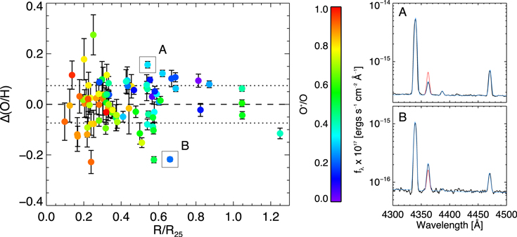
Figure 7. Residuals from the O/H abundance gradient plotted against their R/R25. Each H ii region is color-coded using its derived ratio of O+/O to trace ionization state. We identify two regions which are located at similar radius and have a similar ionization state but which have very different abundances with residuals on opposite sides of the spread. Spectral extractions, focused on the portion of the spectrum containing [O iii] λ4363, for these two regions are shown to the right with data plotted in black and the modeled spectrum shown in blue. The red line indicates the measurement of the [O iii] λ4363 required to fall on the O/H gradient.
Download figure:
Standard image High-resolution imageIn addition to investigating residuals from the O/H gradient with respect to radial location, we consider many other logical candidates for possible second parameters. These include physically motivated parameters, such as the ionization parameter P, and data-driven considerations, for example, the equivalent width of the auroral lines. In Table 7 we give the parameters searched and their associated correlation coefficients. In no cases do any parameters show a significant correlation with the O/H residuals.
Table 4. Abundances in NGC 5457
| NGC 5457–75.0+29.3 | NGC 5457+22.1–102.1 | NGC 5457+47.9–103.2 | NGC 5457–12.0+139.0 | NGC 5457+138.9+30.6 | |
|---|---|---|---|---|---|
| T[O ii]measured (K) | ... | ... | ... | 8110 ± 440 | 7290 ± 180 |
| T[O iii]measured (K) | ... | ... | ... | ... | ... |
| T[N ii]measured (K) | 6300 ± 410 | 6850 ± 440 | 6650 ± 320 | 7320 ± 510 | 7480 ± 310 |
| T[S iii]measured (K) | 5800 ± 400 | ... | ... | ... | 6670 ± 200 |
| n(e)measured (cm−3) | 82 ± 60 | ... | 35 ± 50 | 34 ± 73 | 44 ± 49 |
| T[O ii]used (K) | 6300 ± 410 | 6850 ± 440 | 6650 ± 320 | 7320 ± 510 | 7480 ± 310 |
| T[O iii]used (K) | 5230 ± 290 | 5990 ± 320 | 5720 ± 280 | 6650 ± 360 | 6880 ± 280 |
| T[N ii]used (K) | 6300 ± 410 | 6850 ± 440 | 6650 ± 320 | 7320 ± 510 | 7480 ± 310 |
| T[S iii]used (K) | 5800 ± 400 | 5860 ± 580 | 5600 ± 420 | 6470 ± 670 | 6670 ± 200 |
| n(e)adopted (cm−3) | 100. ± 100. | 100. ± 100. | 100. ± 100. | 100. ± 100. | 100. ± 100. |
| O+/H+ (105) | 32.1 ± 6.2 | 33.1 ± 6.0 | 47.1 ± 6.7 | 24.4 ± 4.4 | 23.6 ± 2.6 |
| O++/H+ (105) | 4.86 ± 0.80 | 7.5 ± 1.1 | 5.30 ± 0.70 | 4.58 ± 0.60 | 4.67 ± 0.40 |
| 12 + log(O/H) (dex) | 8.568 ± 0.074 | 8.609 ± 0.065 | 8.720 ± 0.056 | 8.461 ± 0.067 | 8.452 ± 0.040 |
| N+/H+ (106) | 84 ± 10 | 59.6 ± 7.1 | 75.4 ± 7.2 | 49.0 ± 6.5 | 41.0 ± 3.0 |
| N ICF | 1.15 ± 0.30 | 1.23 ± 0.30 | 1.11 ± 0.20 | 1.19 ± 0.30 | 1.20 ± 0.20 |
| log(N/O) (dex) | −0.580 ± 0.100 | −0.750 ± 0.094 | −0.800 ± 0.074 | −0.700 ± 0.098 | −0.760 ± 0.057 |
| 12 + log(N/H) (dex) | 7.99 ± 0.10 | 7.86 ± 0.10 | 7.924 ± 0.093 | 7.77 ± 0.10 | 7.691 ± 0.069 |
| S+/H+ (107) | 58.1 ± 6.8 | 53.4 ± 5.9 | 53.8 ± 4.6 | 38.7 ± 4.4 | 23.1 ± 1.6 |
| S++/H+ (107) | 120 ± 13 | 65.1 ± 9.9 | 183 ± 22 | 86 ± 13 | 116.1 ± 5.9 |
| S ICF | 1.15 ± 0.30 | 1.23 ± 0.30 | 1.11 ± 0.20 | 1.19 ± 0.30 | 1.20 ± 0.20 |
| log(S/O) (dex) | −1.26 ± 0.10 | −1.45 ± 0.10 | −1.30 ± 0.10 | −1.29 ± 0.10 | −1.230 ± 0.076 |
| 12 + log(S/H) (dex) | 7.31 ± 0.10 | 7.16 ± 0.10 | 7.421 ± 0.093 | 7.17 ± 0.10 | 7.222 ± 0.065 |
| Ne++/H+ (106) | ... | 19.6 ± 5.5 | ... | 10.3 ± 2.6 | 10.8 ± 2.3 |
| Ne ICF | 7.6 ± 1.8 | 5.4 ± 1.1 | 9.9 ± 1.9 | 6.3 ± 1.3 | 6.06 ± 0.80 |
| log(Ne/O) (dex) | ... | −0.60 ± 0.10 | ... | −0.60 ± 0.10 | −0.60 ± 0.10 |
| 12 + log(Ne/H) (dex) | ... | 8.03 ± 0.20 | ... | 7.81 ± 0.10 | 7.82 ± 0.10 |
| Ar++/H+ (107) | 6.9 ± 1.1 | 11.9 ± 3.2 | 18.4 ± 3.2 | 10.3 ± 1.9 | 11.38 ± 0.70 |
| Ar ICF | 3.28 ± 0.50 | 3.77 ± 0.70 | 2.97 ± 0.40 | 3.10 ± 0.50 | 2.54 ± 0.20 |
| log(Ar/O) (dex) | −2.22 ± 0.10 | −1.96 ± 0.20 | −1.98 ± 0.10 | −1.96 ± 0.10 | −1.991 ± 0.061 |
| 12 + log(Ar/H) (dex) | 6.351 ± 0.096 | 6.65 ± 0.10 | 6.738 ± 0.092 | 6.51 ± 0.10 | 6.461 ± 0.046 |
Only a portion of this table is shown here to demonstrate its form and content. A machine-readable version of the full table is available.
Download table as: DataTypeset image
Looking at the 2D distribution of abundances in NGC 5457, we do see a possible mild correlation with the spiral arms, as traced out by the H ii regions. Using the CONTOUR routine in IDL, we interpolate between our irregularly spaced data to create surface maps of oxygen abundance in NGC 5457. We show 2D maps of 12 + log(O/H) in NGC 5457, based on assuming a simple radial gradient (left) and the direct abundances measured in regions where we detect auroral lines (right), in Figure 8. Comparing these two maps shows that deviations from the O/H gradient are relatively localized. Indeed, isolating individual spiral arms in fitting abundance gradients does not significantly diminish the internal dispersion measured. However, care must be taken as comparing the locations of the observed H ii regions (black + signs) to the structure shows that even with 74 regions, sparse sampling clearly affects the derived map.

Figure 8. 2D maps of 12 + log(O/H) in NGC 5457. These maps were created (1) based on assuming a simple projected radial gradient (left), and (2) the "direct" abundances measured in regions where auroral lines were detected (right). Both maps are overlaid on an Hα image. As the number density of direct abundances increase, more structure in gas-phase O/H is clearly apparent.
Download figure:
Standard image High-resolution imageWhile we cannot justify the significant amount of error which must be added to our measurements to eliminate this large amount of scatter, there are other possibilities that remain to be explored. One likely contribution to this scatter is the fact that we have assumed each H ii region is composed of three zones that exist as isothermal slabs as gas-phase entities embedded in the surrounding interstellar medium. This is clearly not a physically accurate description of the system. Rather, as the higher ionization zone is embedded within the lower ionization, there must be, at the very least, a gradual transition of electron temperature across this boundary. Further complicating this picture is the fact that images of H ii regions clearly show they are not smooth Strömgren spheres but show noticeable structure.
The effect of temperature fluctuations in the nebulae affecting estimates of temperatures and hence abundances has been discussed since the pioneering work of Peimbert (1967), who established a formalism to deal with the inhomogeneity of the temperature zones. These thermal inhomogeneities have been estimated to necessitate corrections on the order of 0.15–0.35 dex (Peña-Guerrero et al. 2012), a factor that is larger than the dispersion we see at a given galactocentric radius in our data. In the absence of independent temperature measurements to inform us of the magnitude of this effect from region-to-region, we acknowledge that a global offset of +0.25 dex in O/H may be present in our measurements, with perhaps an additional +0.1 dex to account for possible oxygen depletion onto dust grains (Jenkins 2004). We do not, however, apply such global corrections to the data we present here.
4.2. Enrichment Relative to Oxygen
In Figure 9 we plot N/O, S/O, Ne/O, and Ar/O as a function of O/H. As expected from stellar nucleosynthetic yields (e.g., Woosley & Weaver 1995) and the assumption of a universal initial mass function, these ratios are flat as a function of the radial extent of the galaxy. The S/O, Ar/O, and Ne/O ratios are largely consistent with the constant values observed in massive and low-mass, star-forming galaxies. We note that some of the offset seen between our data (red points) and data culled from the literature is likely due to the adoption of slightly different atomic data and ICFs. Furthermore we note that by using the updated ICFs we do not detect depressed values of Ar/O and S/O in the most metal-rich H ii regions (12 + log(O/H) ≳ 8.75) as reported in Croxall et al. (2015). As seen in other studies, we find increased secondary production of nitrogen at higher O/H (e.g., Vila-Costas & Edmunds 1992). Similar to Croxall et al. (2015) we detect signatures of massive Wolf–Rayet stars in several apertures (see Table 2). However, the presence of features attributed to Wolf–Rayet stars does not appear to lead to any trends of altered abundances.

Figure 9. Relative enrichment of nitrogen and the α elements. Light gray circles represent direct abundances taken from Bresolin et al. (2005, 2009a, 2009b), Croxall et al. (2009), Esteban et al. (2009), Kennicutt et al. (2003), Peimbert et al. (2005), Testor (2001), Testor et al. (2001), Zurita & Bresolin (2012), and Berg et al. (2015). (Top)–(Bottom): log(N/O) as a function of oxygen abundance. The dotted line designates the theoretical curve of Vila-Costas & Edmunds (1992), the black dashed line is the empirical linear fit to galaxies from Pilyugin et al. (2010), the black dotted–dashed curve is the quadratic fit from Pilyugin et al. (2010), the blue dashed line is the scaled model fit from Groves et al. (2004); log (S/O) as a function of oxygen abundance; log (Ne/O) as a function of oxygen abundance; log (Ar/O) as a function of oxygen abundance. In the three lower panels, the dashed line in each panel denotes the mean value for our observations of NGC 5457. Additionally, we have marked the locus of the population of H ii regions with log(Ne/O) ≈ −1.0 using a dashed red line.
Download figure:
Standard image High-resolution imageTable 5. Comparison with Previous Observations
| H ii Region |

|
[O iii] λ5007 | [O iii] λ4363 | [N ii] λ5755 | [S iii] λ6312 | T[O iii] | T[N ii] | T[S iii] | 12 + log( ) ) |
log( ) ) |
log( ) ) |
|---|---|---|---|---|---|---|---|---|---|---|---|
| −75.0+29.3 | 0.10 | 6 | ... | 0.32 | 0.22 | ... | 6306 | 5806 | 8.56 | −0.58 | −1.26 |
| H493 (B07)a | 0.10 | 8 | ... | 0.24 | 0.27 | ... | 5960 | 7330 | 8.74 | 0.72 | −1.78 |
| +164.6+9.9 | 0.20 | 98 | 0.20 | 0.44 | 0.79 | 7422 | 7673 | 6910 | 8.57 | −0.96 | −1.23 |
| H1013 (K03) | 0.19 | 103 | ... | 0.50 | 0.80 | ... | 8040 | 6705 | 8.47 | −0.90 | −1.04 |
| H1013 (B07) | 0.19 | 102 | 0.24 | 0.59 | 0.77 | 7656 | 8225 | 7512 | 8.48 | −0.91 | −1.34 |
| −159.9+89.6 | 0.22 | 19 | ... | 0.51 | 0.35 | ... | 7140 | 5969 | 8.55 | 0.77 | −1.22 |
| H336 (K03) | 0.22 | 23 | ... | 0.50 | 0.60 | ... | 7121 | 6557 | 8.61 | −0.82 | −1.29 |
| +254.6-107.2 | 0.33 | 346 | 1.39 | 0.40 | 1.54 | 8739 | 8931 | 9344 | 8.48 | −1.00 | −1.58 |
| H1105 (K03) | 0.34 | 316 | 1.40 | 0.40 | 1.30 | 8949 | 9380 | 7867 | 8.42 | −1.08 | −1.27 |
| +354.1+71.2 | 0.43 | 352 | 1.94 | 0.37 | 1.40 | 9542 | 9079 | 8192 | 8.45 | −1.20 | −1.17 |
| H1170 (K03)a | 0.42 | 201 | 1.60 | ... | 1.70 | 10800 | ... | 8500 | 8.37 | 1.20 | 1.44 |
| +360.9+75.3 | 0.44 | 354 | 1.71 | ... | 1.28 | 9179 | ... | 8027 | 8.43 | −1.18 | −1.34 |
| H1176 (K03) | 0.43 | 369 | 2.40 | ... | 1.50 | 9993 | ... | 8586 | 8.30 | −1.16 | −1.27 |
| −99.6-388.0 | 0.47 | 388 | 2.08 | 0.36 | 1.41 | 9443 | 9940 | 8925 | 8.38 | −1.15 | −1.47 |
| H409 (K03) | 0.48 | 370 | 2.30 | 0.40 | 1.70 | 9858 | 10160 | 9861 | 8.33 | −1.17 | −1.51 |
| −226.9-366.4 | 0.50 | 151 | 0.89 | 0.73 | 1.28 | 9705 | 11120 | 9288 | 8.18 | −1.18 | −1.27 |
| H219 (Li13) | 0.50 | 178 | 0.91 | ... | ... | 9319 | ... | ... | 8.51 | −1.43 | ... |
| −368.3-285.6 | 0.54 | 323 | 1.64 | 0.43 | 1.40 | 9299 | 9381 | 11150 | 8.42 | −1.13 | −1.54 |
| H149 (Li13) | 0.54 | 329 | 1.68 | ... | ... | 9309 | ... | ... | 8.46 | −1.20 | ... |
| H149 (K03) | 0.55 | 318 | 1.80 | 0.90 | 1.40 | 9588 | 13050 | 8925 | 8.37 | −1.08 | −1.17 |
| −371.1-280.0 | 0.54 | 267 | 1.61 | 0.48 | 1.28 | 9768 | 9625 | 11110 | 8.33 | −1.13 | −1.52 |
| H143 (K03) | 0.55 | 284 | 2.30 | 0.90 | 1.40 | 10711 | 13600 | 8992 | 8.18 | −1.06 | −1.05 |
| −455.7-55.8 | 0.55 | 325 | 2.92 | ... | 1.28 | 11080 | ... | 12080 | 8.22 | −1.43 | −1.61 |
| H59 (Li13) | 0.55 | 290 | 2.30 | ... | ... | 10640 | ... | ... | 8.30 | −1.54 | ... |
| −392.0-270.1 | 0.55 | 372 | 2.10 | 0.29 | 1.31 | 9578 | 9553 | 11200 | 8.35 | −1.14 | −1.80 |
| H128 (K03) | 0.56 | 391 | 1.70 | 0.30 | 1.30 | 8904 | 10100 | 8405 | 8.42 | −1.10 | −1.32 |
| −455.7-55.8 | 0.55 | 325 | 2.92 | ... | 1.28 | 11080 | ... | 12080 | 8.22 | −1.43 | −1.61 |
| H67 (K03) | 0.56 | 342 | 3.50 | ... | 1.80 | 11610 | ... | 10040 | 8.14 | −1.38 | −1.12 |
| −453.8-191.8 | 0.58 | 374 | 3.64 | 0.32 | 1.44 | 11390 | 10710 | 14510 | 8.21 | −1.37 | −1.67 |
| H71 (K03) | 0.57 | 454 | 5.90 | ... | 1.90 | 12690 | ... | ... | 8.06 | −1.26 | ... |
| −481.4-0.5 | 0.58 | 284 | 3.92 | ... | 1.31 | 12970 | ... | 14920 | 8.02 | −1.37 | −1.61 |
| H27 (Li13) | 0.58 | 251 | 3.64 | ... | ... | 13260 | ... | ... | 8.01 | −1.39 | ... |
| +315.3+434.4 | 0.62 | 441 | 3.67 | ... | ... | 10810 | ... | ... | 8.32 | −1.31 | −1.40 |
| H1146 (Li13) | 0.63 | 457 | 3.07 | ... | ... | 10090 | ... | ... | 8.40 | −1.40 | ... |
| +509.5+264.1 | 0.67 | 417 | 3.37 | 0.25 | 1.53 | 10690 | 10350 | 9933 | 8.26 | −1.33 | −1.52 |
| H1216 (K03) | 0.67 | 473 | 4.70 | ... | 1.60 | 11490 | ... | 9982 | 8.17 | −1.34 | −1.40 |
| +667.9+174.1 | 0.81 | 674 | 8.85 | 0.16 | 1.64 | 12790 | 11150 | 12110 | 8.14 | −1.37 | −1.65 |
| N5471-A (K03) | 0.81 | 644 | 9.50 | ... | 1.60 | 13354 | ... | 11500 | 8.05 | −1.35 | −1.43 |
| +1.0+885.8 | 1.05 | 184 | 2.72 | ... | ... | 13350 | ... | ... | 7.85 | −1.47 | −1.59 |
| H681a (K03) | 1.04 | 312 | 5.00 | ... | ... | 13820 | ... | ... | 7.91 | −1.51 | −1.55 |
| H681 (Li13) | 1.05 | 260 | 4.36 | ... | ... | 14100 | ... | ... | 7.85 | −1.55 | ... |
Notes. H ii regions that are in common between our new observations and Kennicutt et al. (2003), Bresolin (2007), and Li et al. (2013). For each H ii region we give the offset from the galaxy center given in Table 1 on the first line along with the derived results from this study. In the subsequent lines for each given region, we report the name used in the comparison study as well as give an abbreviated name for each study, namely, K03 for Kennicutt et al. (2003), B07 for Bresolin (2007), and L13 for Li et al. (2013). Fluxes are given in units of Hβ = 100.
aThese regions are compared to the published values from Kennicutt et al. (2003) and Bresolin (2007) as discussed in the text.Download table as: ASCIITypeset image
While the bulk Ne/O trend is indeed flat, there exists a population of H ii regions with a significant offset to low values of Ne/O, i.e., log(Ne/O) ≈ −1 (see Figures 6 and 9). The existence of two populations of Ne/O, rather than simply a large spread in a single population, is confirmed using a nonparametric kernel technique that does not presuppose an a priori shape to the distribution (Vio et al. 1994; Ryden 2006). H ii regions that exhibit low Ne/O do not display unusual deficits in other relative abundances, e.g., O/H, N/O, S/O, or Ar/O, and span the full range of O/H we have measured. These regions are not isolated in a specific location in NGC 5457, nor are they correlated with the presence of unusual features, such as Wolf–Rayet features or narrow He ii emission, in the spectra.
We note that in our derivation of Ne abundances we have used only the isolated [Ne iii] λ3868 line; thus, the low abundances cannot be attribution to errors in de-blending the [Ne iii] λ3967 line with the nearby H7 line. Furthermore, Figure 9 shows that similar values of Ne/O are not uncommon in the literature. However, the reduction in measurement uncertainty permitted by the CHAOS data reveal these regions to be a second population and not simply statistical outliers.
5. CONCLUSIONS
Leveraging the the power of the LBT with the broad spectral range and sensitivity of MODS, we have measured uniform "direct" abundances in a large sample of H ii regions in spiral galaxies as part of the CHAOS project. Here we highlight our observations of 101 H ii regions in NGC 5457 (M101), with a specific focus on the 74 regions where we detected at least one of the temperature-sensitive auroral lines of either [O iii], λ4363, [N ii], λ5755, or [S iii], λ6312. In 55 cases, more than 1 of these innately faint emission lines were detected, permitting a comparison of multiple temperature measurements.
The detection of multiple auroral lines in numerous H ii regions allows us to explore the correlations between the different derived ionic temperature zones. We have found (1) strong correlations of T[N ii] with T[S iii] and T[O iii], consistent with little or no intrinsic dispersion and the predictions of photoionization modeling; (2) a correlation of T[S iii] with T[O iii], but with significant dispersion and significantly different from the prediction of photoionization modeling; (3) overall agreement between T[N ii], T[S ii], and T[O ii] as expected, but with significant dispersion.
Given these numerous detections of lines, particularly in the less explored low-ionization regime, i.e., O+/O > 0.4, we inspect the commonly used ICFs. Unfortunately, many of the common ICFs are found to be deficient in this region of parameter space. We propose new empirical ICFs for S and Ar based on our large uniform data set.
One additional reason we targeted NGC 5457 was to permit a robust comparison with the data of Kennicutt et al. (2003), Bresolin (2007), and Li et al. (2013). We show that our pipelines produce results that are in very good agreement with the older data, when updated atomic data are taken into consideration. Furthermore, our MODS spectra show that some of the unusual temperatures measured in Kennicutt et al. (2003) can be rectified with the higher signal-to-noise of our data. On the other hand, we also detect clear evidence that some unusual temperatures are not due to the difficulty of measuring innately weak lines.
We measure abundance gradients in both O/H and N/O that are in good agreement with the previous measurements in the literature, namely a steep gradient that drops from approximately solar neighborhood metallicity in the center of NGC 5457 (Nivea & Przybilla 2012). At R/R25 ≈ 0.7 we detect a clear flattening of the N/O gradient signaling the low-metallicity outer regions of NGC 5457 are dominated by primary production of N. We fit these abundance gradients using a Markov-Chain Monte Carlo approach that includes the possibility that intrinsic dispersion is present. Despite different dependencies on temperature, both O/H and N/O gradients show the presence of significant internal dispersion at a given radius, namely, 0.074 ± 0.009 dex and 0.095 ± 0.009 dex, respectively. Furthermore, we have shown that this dispersion is not related to ionization or other likely second parameters measured from the spectra or their location in the galaxy but appears to be somewhat stochastic.
In contrast, Ne/O, Ar/O, and S/O all exhibit flat trends with O/H consistent with no evolution of these abundance ratios across the entire disk of NGC 54557. While the median value of Ne/O is indeed constant with O/H, we discover a population of H ii regions with a significant offset to low values in Ne/O, ∼−1. This population is present across the range of ionization parameters and abundance trends measured. Comparing Ne/O measurements from CHAOS with those from the literature show that other galaxies likely have similar populations of low Ne/O, but the number of observations was too small to robustly detect a separate population.
As the locations of ongoing star formation, spiral galaxies are where we can observe the chemical evolution of out universe unfolding. However, only with the advent of very sensitive multi-object spectrographs have we been able to measure the requisite features necessary to truly map out the patterns of the evolution. These observations are vital in understanding the origin of the elements and their role in the shaping galaxies and the universe as we see it.
K.V.C. is grateful for support from NSF Grant AST-6009233. K.V.C. is extremely grateful for the chance to have worked with the MODS spectrograph and the CHAOS team. We thank the anonymous referee for useful comments that helped improve the manuscript. This paper uses data taken with the MODS spectrographs built with funding from NSF grant AST-9987045 and the NSF Telescope System Instrumentation Program (TSIP), with additional funds from the Ohio Board of Regents and the Ohio State University Office of Research. This paper made use of the modsIDL spectral data reduction pipeline developed in part with funds provided by NSF Grant AST-1108693. We are grateful to D. Fanning, J.X. Prochaska, J. Hennawi, C. Markwardt, M. Williams, and others who have developed the IDL libraries of which we have made use: coyote graphics, XIDL, idlutils, MPFIT, and impro. This work was based in part on observations made with the Large Binocular Telescope (LBT). The LBT is an international collaboration among institutions in the United States, Italy, and Germany. The LBT Corporation partners are: the University of Arizona on behalf of the Arizona university system; the Istituto Nazionale di Astrofisica, Italy; the LBT Beteiligungsgesellschaft, Germany, representing the Max Planck Society, the Astrophysical Institute Potsdam, and Heidelberg University; the Ohio State University; and the Research Corporation, on behalf of the University of Notre Dame, the University of Minnesota, and the University of Virginia. This research has made use of the NASA/IPAC Extragalactic Database (NED) which is operated by the Jet Propulsion Laboratory, California Institute of Technology, under contract with the National Aeronautics and Space Administration.
Facility: LBT(Multi-Object Double Spectrograph 1). -
Softwares: Astropy (Robitaille et al. 2013), linmix (Kelly 2007, https://githubcom/jmeyers314/linmix), STARLIGHT (Cid Fernandes et al. 2005).
APPENDIX: IONIZATION CORRECTION FACTORS
A.1. Nitrogen
Nitrogen abundances were derived under the assumption that

This assumption has been well tested in low-abundance nebulae (Garnett 1990). Unfortunately, its validity is less certain in higher abundance spiral galaxies. We note that combining observations of the ultraviolet N iii] and the far-IR [N iii] 57 μm line with the now large sample of metal-rich H ii regions with optically measured N+/O+ would be greatly beneficial in establishing the veracity of this assumption in cool metal-rich environments.
We note that the work of Nava et al. (2006) suggest that the nitrogen ICF should have a scale factor of 1.08 ± 0.09 rather than that of unity. While we have not adopted this scale factor at this time, we note that its adoption does not alter any conclusions and merely results in a simple increase of all reported log(N/O) values by 0.03 dex.
Table 6. N/O in NGC 5457
| T[N ii](adopted) | log(N/O) | |
|---|---|---|
| (K) | (dex) | |
| NGC 5457+134.8+146.0 | 7306 ± 1000 | −0.72 ± 0.20 |
| NGC 5457–52.1+41.2 | 6702 ± 1000 | −0.62 ± 0.20 |
| NGC 5457–96.2–68.7 | 7239 ± 1000 | −0.68 ± 0.20 |
| NGC 5457–190.6–10.8 | 7642 ± 1000 | −0.74 ± 0.20 |
| NGC 5457–139.7–157.6 | 7642 ± 1000 | −0.77 ± 0.20 |
| NGC 5457–70.6–92.8 | 6500 ± 1000 | −0.56 ± 0.20 |
| NGC 5457–22.0+1.6 | 6030 ± 1000 | −0.48 ± 0.20 |
| NGC 5457+20.0–104.4 | 7172 ± 1000 | −0.69 ± 0.20 |
| NGC 5457–203.8–135.6 | 8180 ± 1000 | −0.89 ± 0.20 |
| NGC 5457–205.2–128.7 | 8650 ± 1000 | −0.92 ± 0.20 |
| NGC 5457–226.8–77.8 | 8718 ± 1000 | −0.93 ± 0.20 |
| NGC 5457+68.2+161.8 | 7038 ± 1000 | −0.66 ± 0.20 |
| NGC 5457+44.7+153.7 | 7239 ± 1000 | −0.65 ± 0.20 |
| NGC 5457–44.1+149.5 | 6903 ± 1000 | −0.63 ± 0.20 |
| NGC 5457–123.1+146.1 | 7508 ± 1000 | −0.77 ± 0.20 |
| NGC 5457–192.5+124.7 | 8180 ± 1000 | −0.84 ± 0.20 |
| NGC 5457+7.2–3.8 | 6298 ± 1000 | −0.40 ± 0.20 |
| NGC 5457–222.9–366.4 | 9994 ± 1000 | −1.37 ± 0.20 |
| NGC 5457–133.9–178.7 | 8314 ± 1000 | −0.91 ± 0.20 |
| NGC 5457–66.9–210.8 | 7105 ± 1000 | −0.73 ± 0.20 |
| NGC 5457+299.1+464.0 | 9860 ± 1000 | −1.09 ± 0.20 |
| NGC 5457–209.1+311.8 | 9591 ± 1000 | −1.01 ± 0.20 |
| NGC 5457–219.4+308.7 | 9457 ± 1000 | −1.05 ± 0.20 |
| NGC 5457–225.0+306.6 | 8986 ± 1000 | −1.01 ± 0.20 |
| NGC 5457–167.8+321.5 | 9860 ± 1000 | −1.23 ± 0.20 |
Note. N/O abundances for regions where no auroral lines were measured. This ratio is insensitive to the temperature adopted; nevertheless, we report the adopted semi-empirical temperature.
Download table as: ASCIITypeset image
A.2. Neon
Similar to nitrogen, neon can only be measured in one ionization state in optical nebulae. Peimbert & Costero (1969) suggested that neon abundance could be derived under the assumption

As neon is significantly stronger in high-ionization nebula, it has predominantly been measured in low-abundance nebula. In pushing toward neon measurements in low-ionization nebula, Kennicutt et al. (2003) noted that the scatter in Ne++/O++ increased at higher O+/O. This could indicate that the neon ICF does significantly change as H ii regions become cooler. Dors et al. (2013) revisited the ionization fraction of neon by using mid-IR observations of [Ne ii] and [Ne iii] to directly measure the neon ionization fraction. However, they note that the overlap between visible and IR measurements of neon is limited to more metal-poor regions.
Given the sensitivity of the MODS1 spectrograph, we are able to detect the [Ne iii] λ3869 line in 40 H ii regions with a 12 + log(O/H) ≥ 8.4. In Figure 10 we show the ratio of Ne++/O++ as a function of the ionization fraction of oxygen, O+/O. In addition to the Peimbert & Costero (1969) relation, we also plot the two ICFs derived by Dors et al. (2013),

and
where

normalized to a constant log(Ne/O) = −0.70.
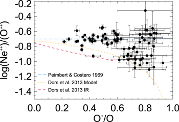
Figure 10. Ratio of Ne++/O++ as a function of the ionization fraction of oxygen, O+/O for H ii regions in NGC 5457. We also include the ionization corrections fractions derived by Dors et al. (2013).
Download figure:
Standard image High-resolution imageThe majority of our data are indeed consistent with a constant ratio across a wide range of ionization. Compared to Equation (13), both ICFs derived by Dors et al. (2013) appear to underpredict the amount of Ne relative to oxygen. Indeed, adopting the ionization correction of Peimbert & Costero (1969) for neon yields agreement with the IR measurements of Dors et al. (2013), a constant Ne/O ratio at log(Ne/O) = −0.70.
However, we see a related phenomena to the increased scatter at higher O+/O reported by Kennicutt et al. (2003) in our significantly larger data set, 42 regions in this portion of parameter space compared to 2 regions. Ne++/O++ appears to bifurcate and inhabit either a high or a low ratio, both of which are flat as a function of O+/O. It is worth noting that the cluster at Ne++/O++ ∼ 1.0 appears to agree more closely with the results from IR data (Dors et al. 2013). Given the quality of the spectra, we rule out measurement error as a cause for the low values of Ne++/O++. Furthermore, we note that only the [Ne iii] λ3869 line has been used; thus, this cannot be attributed to blended lines that have skewed the measurement of the [Ne iii] λ3967 line, which does give consistent results.
Table 7. Possible Second Parameters in the O/H Abundance Gradient
| Correlation Coefficients | |||
|---|---|---|---|
| r | ρ | τ | |
| P | 0.22 | 0.29 | 0.19 |
| O+/O | −0.23 | −0.30 | −0.19 |
| [O iii] λ5007 | 0.21 | 0.27 | 0.18 |
| [N ii] λ6583 | −0.02 | −0.07 | −0.05 |
| Hα/Hβ | 0.13 | 0.12 | 0.08 |
| [O iii]/[O ii] | 0.25 | 0.29 | 0.19 |
| R23 | 0.17 | 0.23 | 0.16 |
| LHβ | −0.06 | 0.11 | 0.08 |
| EWHβ | 0.26 | 0.28 | 0.19 |
| EW4363 | 0.28 | 0.29 | 0.20 |
| EW5755 | 0.28 | 0.30 | 0.20 |
| Δ(N/O) | −0.12 | 0.07 | 0.11 |
| R/R25 | −0.01 | 0.07 | 0.04 |
| ϕ | 0.06 | 0.09 | 0.06 |
Note. Coefficients from Pearson's (r), Spearmans (ρ), and Kendall's (τ) rank correlation of residuals from the O/H gradient and other plausible second parameters.
Download table as: ASCIITypeset image
For this work we choose to use the ionization correction formula from Peimbert & Costero (1969), i.e., Equation (13). However, we note that this result is more robust in metal-poor H ii regions that are characterized by high-ionization parameters. Indeed, the mid-IR lines in metal-rich regions warrant more investigation once the JWST is active.
A.3. Sulfur
While both S+ and S++ are observed in our spectra, we must account for the presence of S+3 (30.2 eV) in the highly ionized region (Garnett 1989). An analytical ICF for sulfur has been reported by Thuan et al. (1995), based on the photoionization modeling of Stasińska (1990),
where x is again defined in (11). This correction is in practice similar to that adopted by Kennicutt et al. (2003) based on earlier photoionization models (Stasińska 1978):
with α = 2.5. We show these two relations as dashed blue (Kennicutt et al. 2003) and dotted red (Thuan et al. 1995) lines, along with our data in Figure 11 for an assumed (constant) intrinsic log(S/O) = −1.60. While our data do not explore the parameter space of highly ionized regions (i.e., O+/O ≤ 0.2) compared to previous works, they more thoroughly populate the low-ionization region revealing a clear trend with the oxygen ionization fraction that is not seen in the models. We also note that atomic data for sulfur has been significantly revised in recent years. This change in atomic data alone can account for a shift of ≈0.1 dex between the reported values of (S+ + S++)/(O+ + O++) and those derived by models using older atomic data.

Figure 11. Left: the ratio of (S+ + S++)/(O+ + O++) as a function of the ionization fraction of oxygen, O+/O for H ii regions in NGC 5457. We also include the ionization corrections fractions derived by Thuan et al. (1995) and Kennicutt et al. (2003). Right: the ratio of (S+ + S++)/(O+) as a function of the ionization fraction of oxygen.
Download figure:
Standard image High-resolution imageComparing the ionization potentials of the observed sulfur ions, S+ (10.4 eV) and S++ (23.3 eV), with the observed oxygen ions, O+ (13.6 eV) and O++ (35.1 eV), suggests that singly ionized oxygen may be a better tracer of the sulfur in cooler H ii regions. This is clearly illustrated in the right panel of Figure 11, where the ratio (S+ + S++)/O+ is constant for O+/O ≥ 0.4. This ratio was previously adopted as an ICF for sulfur (Peimbert & Costero 1969). However, Pagel (1978) noted a correlation with O+/O in the observed H ii regions at the time. While we do detect this correlation, the larger data set, which is in agreement with the data of Pagel (1978), shows that the correlation is limited to high-ionization H ii regions.
Adopting the Thuan et al. (1995) or Kennicutt et al. (2003) ICFs for sulfur results in a significant trend in S/O with O+/O, whereas (S+ + S++)/O+ indicates this ratio should be flat (Garnett 1989). Therefore, we adopt

for O+/O ≥ 0.4 and the ionization correction of Thuan et al. (1995) for O+/O ≤ 0.4
A.4. Argon
Similar to neon, only one ionization state is observed. However, like sulfur, in most nebular conditions, three ionization states can be present: Ar+ in low-ionization zones and Ar+3 in the highly ionized portions of the nebulae. Given that the ionization potentials of sulfur and oxygen ions bracket the respective energy levels in argon ions, ratios with both elements have been used to trace the unseen argon.
In Figure 12 (left panel), we show the ratio of Ar++/O++ as a function of O+/O along with the ICF of Thuan et al. (1995),

where x is again defined in (11), for an assumed (constant) intrinsic log(Ar/O) = −2.20. In agreement with Kennicutt et al. (2003), we find that this ratio is strongly correlated with the ionic fraction of oxygen and is thus a poor predictor of Ar/O. We also show the ratio of Ar++/S++ as a function of O+/O in Figure 12 (right panel). Kennicutt et al. (2003) found this ratio to be uncorrelated with O+/O and, aside from a single low-ionization region, to exhibit a constant value, log(Ar++/S++) = −0.60. Our sample clearly shows that low-ionization regions do not maintain a constant value of Ar++/S++ rendering it insufficient as a sole representative of Ar/S.

Figure 12. Left: the ratio of Ar++/O++ as a function of the ionization fraction of oxygen, O+/O for H ii regions in NGC 5457. We also include the ionization corrections fraction derived by Thuan et al. (1995). Right: the ratio of Ar++/O++ as a function of the ionization fraction of oxygen.
Download figure:
Standard image High-resolution image
To correct for the decrease in Ar++/S++ in low-ionization nebula, we adopt a linear correction to Ar++/S++,

to account for an increase in the Ar+ population before adopting this ratio as representative of the Ar/S ratio, with an uncertainty of ≈±0.1 dex. To fully explore the validity of this assumption, observations of the 70 μm [Ar ii] line are needed. Currently, this line is only accessible with the SOFIA observatory.
Footnotes
- 6
- 7
- 8
- 9