


ABSTRACT
Lambda Boo-type stars are a group of late B to early F-type Population I dwarfs that show mild to extreme deficiencies of iron-peak elements (up to 2 dex), but their C, N, O, and S abundances are near solar. This intriguing stellar class has recently regained the spotlight because of the directly imaged planets around a confirmed Lambda Boo star, HR 8799, and a suggested Lambda Boo star, Beta Pictoris. The discovery of a giant asteroid belt around Vega, another possible Lambda Boo star, also suggests hidden planets. The possible link between Lambda Boo stars and planet-bearing stars motivates us to study Lambda Boo stars systematically. Since the peculiar nature of the prototype Lambda Boötis was first noticed in 1943, Lambda Boo candidates published in the literature have been selected using widely different criteria. In order to determine the origin of Lambda Boo stars' unique abundance pattern and to better discriminate between theories explaining the Lambda Boo phenomenon, a consistent working definition of Lambda Boo stars is needed. We have re-evaluated all published Lambda Boo candidates and their available ultraviolet and visible spectra. In this paper, using observed and synthetic spectra, we explore the physical basis for the classification of Lambda Boo stars, and develop quantitative criteria that discriminate metal-poor stars from bona fide Lambda Boo stars. Based on these stricter Lambda Boo classification criteria, we conclude that neither Beta Pictoris nor Vega should be classified as Lambda Boo stars.
Export citation and abstract BibTeX RIS
1. INTRODUCTION
The Lambda Boo class is a subgroup of late B to early F-type stars that have an unusually low abundance of iron-peak elements in their surface layers. The prototype, Lambda Boötis (HD 125162; A3 V), was first reported as peculiar by Morgan et al. (1943). Subsequently, Baschek & Searle (1969) defined the Lambda Boo class as stars whose abundance pattern resembles that of the prototype. Several definitions of Lambda Boo stars are found in the literature (Paunzen 2004). Both photometric and spectroscopic criteria have been used. Some of these criteria are not capable of discriminating Lambda Boo stars from other chemically peculiar stars. For example, although Mg ii lines are generally weak in Lambda Boo stars, most Ap and Am stars also have weak Mg ii 4481 Å lines (Abt & Willmarth 2000). According to various definitions found in the literature, the common characteristic of Lambda Boo stars is the weakness of metallic lines. One theory is that their surface metal abundances have been diluted by the accretion of metal-depleted circumstellar or interstellar gas (Waters et al. 1992), but the cause of the peculiar abundances and the evolutionary status of Lambda Boo stars are still uncertain and subject to debate. In order to determine the origin of Lambda Boo stars' peculiar abundances and to better discriminate between theories explaining the Lambda Boo phenomenon, a quantitative classification scheme for Lambda Boo stars is needed. We have re-evaluated over 200 published Lambda Boo candidates (Murphy et al. 2015) and their existing data to determine whether they exhibit the visible and UV characteristics of Lambda Boo stars.
One of the distinguishing characteristics in a Lambda Boo star's visible spectrum is the overall weakness of the metallic-line spectrum. Gray and Corbally enumerated the optical characteristics of the class in their book "Stellar Spectral Classification" (Gray & Corbally 2009), which we summarize as: "The Lambda Boo stars are A-type Population I dwarfs that show mild to extreme deficiencies of iron-peak elements (although C, N, O, and S can be near solar). MK classification criteria include broad hydrogen lines, a weak metallic-line spectrum compared to MK standards, coupled with a particularly weak Mg ii 4481 Å line." However, many peculiar types near A0 and shell stars also have weak 4481 Å lines (see Ch. 5 of Gray & Corbally 2009). To confirm a star as a Lambda Boo star, it is necessary to verify that it has an elemental abundance pattern similar to Lambda Boo (not just overall metal weak).
The UV region is critical for the classification of Lambda Boo stars because the relative strengths of the C i lines and numerous metal lines can provide a more sensitive and less ambiguous criteria than available in visible spectra. In the ultraviolet, Lambda Boo stars have significantly higher absolute fluxes than normal A-type stars of the same spectral type/effective temperature (see Section 4.3). This is caused by differences in metallic-line blanketing and continuous opacity by metals. Taken alone, these high UV fluxes suggest a significantly higher Teff and an earlier spectral type than the values determined using the visible band. To date, the nature of the UV excess has not been fully studied, and UV classification criteria for Lambda Boo stars have been based on absorption line ratios and a broad spectral feature centered around 1600 Å. The UV classification criteria proposed so far in the literature are mostly equivalent width ratios involving lines shortward of 1700 Å (Faraggiana et al. 1990; Solano & Paunzen 1998, 1999). They are suitable only for hot Lambda Boo stars that have significant flux below 1700 Å. Ohanesyan (2008) demonstrates that the peculiar A-type stars, including Lambda Boo stars, can be identified by analyzing the equivalent width of the 2786–2810 Å spectral band as a function of effective temperature. Although clearly separated from the normal (standard) stars, Lambda Boo stars cannot be distinguished from horizontal branch or other metal-poor stars with International Ultraviolet Explorer (IUE) spectra at wavelengths longer than 1700 Å.
Lambda Boo stars clearly form a separate group among the classical chemically peculiar objects of the upper Main Sequence, as their under-abundance patterns are quite outstanding. Heiter (2002) draws conclusions about the abundance pattern of the group, investigates their statistical properties, and compares the abundances with the interstellar medium. Paunzen (2004) presents a comprehensive overview of the Lambda Boo stars, which covers basic membership criteria as well as existing theories to explain the Lambda Boötis phenomenon.
Excluding C, N, O, and S (which tend to be near solar), Lambda Boo-type stars display a range of metallicities ([M/H]) from −0.50 to −2.03 dex (see Tables 1 and 3). We seek to understand the cause of this distinctive pattern. Therefore, the classification criteria should be based on the relative strength of light and heavy elements. Using both observed and synthetic spectra we can explore the physical basis for the classification of Lambda Boo stars.
Table 1. Program Lambda Boo Stars with IUE Observations
| Identification | Mean Teff | Teff Differencea | [Fe/H] | [M/H] | IUE SWP | IUE LWP/LWR |
|---|---|---|---|---|---|---|
| (K) | (K) | (.mxhi/.mxlo)b | (.mxhi/.mxlo)b | |||
| HD 141569 | 10260 (2), (19), (33), (34) | −260/+240 | −0.50 (1) | ⋯ | x/54330 | 30407/30408 |
| HD 101412 | 10153 (2), (3), (34) | −193/+347 | −1.0 (2) | ⋯ | ⋯ | x/20657 |
| HD 170680 | 9774 (4), (11), (35) | −151/+226 | −0.4 (11) | ⋯ | 28341/x | 08223/x |
| HD 36726 | 9542 (5), (9), (35) | −222/+258 | −0.58 (5) | ⋯ | ⋯ | x/14896 |
| HD 37411 | 9100 (3) | −0/+0 | ⋯ | −1.5 (32) | ⋯ | 21564/x |
| HD 183324 | 9050 (4), (9), (15), (16) | −350/+250 | −1.24 (39) | −1.80 (28) | 28342/50401 | 08220/x |
| HD 171948 A/B | 9011 (23), (35) | −11/+11 | −1.6 (11) | ⋯ | x/48077 | ⋯ |
| HD 110411 | 8975 (9), (10), (11), (13) | −175/+225 | −1.0 (11) | ⋯ | 43603/19125 | 07658/15143 |
| HD 31295 | 8871 (4), (9), (10), (14), (16) | −96/+119 | −0.89 (16) | −1.24 (21) | 17885/17884 | 02557/14124 |
| HD 221756 | 8733 (4), (9), (10), (13), (14) | −223/+287 | −0.64 (14) | −0.75 (28) | 21944/46038 | 02559/x |
| HD 125162 | 8700 (9), (12), (13), (17) | −50/+29 | −2.05 (17) | −2.00 (28) | 17873/17871 | 14117/25220 |
| HD 319 | 8348 (9), (14), (15), (16) | −328/+294 | −0.35 (14) | ⋯ | x/48071 | ⋯ |
| HD 204041 | 8239 (8), (15), (16) | −239/+378 | −0.44 (14) | −0.83 (25) | x/46040 | ⋯ |
| HD 192640 | 7988 (9), (16), (24) | −45/+42 | −2.0 (24) | ⋯ | 43131/44622 | 02100/13712 |
| HD 101108 | 7979 (22), (27), (37) | −79/+109 | −0.60 (11) | ⋯ | x/21396 | x/02171 |
| HD 30422 | 7977 (9), (22), (35), (37) | −107/+210 | ⋯ | −0.52 (25) | x/46036 | ⋯ |
| HD 11413 | 7956 (10), (31), (33), (35) | −31/+42 | −1.5 (10) | −2.03 (29) | x/43608 | ⋯ |
| HD 290799 | 7864 (6), (9), (33), (35) | −151/+136 | −0.97 (5) | ⋯ | x/53844 | x/31912 |
| HD 111604 | 7798 (5), (13), (35) | −198/+202 | −1.08 (5) | −0.75 (28) | x/38239 | ⋯ |
| HD 105058 | 7725 (4), (5), (9) | −95/+75 | −1.20 (5) | −0.64 (30) | x/19129 | 11967/11966 |
| HD 210111 | 7521 (10), (12), (33), (35), (37) | −71/+72 | −1.1 (10) | −1.0 (38) | x/49047 | ⋯ |
| HD 111786 | 7500 (4), (15), (16) | −50/+49 | −1.45 (39) | −0.58 (30) | 43606/19124 | 03557/15142 |
| HD 139614 | 7500 (2), (18) | −100/+100 | −0.5 (2) | ⋯ | x/54332 | x/30412 |
| HD 109738 | 7491 (8), (9), (35) | −70/+112 | −0.83 (8) | −0.92 (25) | x/49728 | ⋯ |
| HD 75654 | 7341 (9), (25), (35), (37) | −81/+90 | ⋯ | −0.95 (25) | x/52691 | x/29429 |
| HD 6870 | 7337 (9), (25), (35) | −97/+107 | ⋯ | −1.08 (25) | x/21334 | x/02117 |
| HD 142703 | 7231 (4), (9), (15), (16), (20) | −31/+30 | −1.10 (14) | ⋯ | 48197/48078 | ⋯ |
| HD 15165 | 7157 (7), (9) | −143/+143 | −0.46 (7) | ⋯ | x/13353 | 10003/x |
| HD 15164 | 7100 (7) | −0/+0 | −0.08 (7) | ⋯ | ⋯ | x/10004 |
| HD 142994 | 7010 (8), (9), (35) | −60/+72 | −0.56 (8) | −0.88 (25) | x/50405 | x/28818 |
| HD 106223 | 6769 (5), (11), (35), (36) | −269/+231 | −1.44 (11) | ⋯ | x/08720 | x/02873 |
| HD 4158 | 6483 (22), (25), (26) | −83/+67 | −0.17 (35) | −1.59 (25) | x/21388 | x/02164 |
Notes.
aThe difference between the mean effective temperature and the lowest/highest effective temperature. bMXHI stands for High-Dispersion Merged Extracted Image FITS File. MXLO stands for Low-Dispersion Merged Extracted Image FITS File.References. (1) Merín et al. (2004), (2) Guimarães et al. (2006), (3) Maaskant et al. (2014), (4) Solano & Paunzen (1999), (5) Andrievsky et al. (2002), (6) Faraggiana et al. (1997), (7) Andrievsky et al. (1995), (8) Solano et al. (2001), (9) Paunzen et al. (2002a), (10) Sturenburg (1993), (11) Heiter (2002), (12) Paunzen et al. (2003), (13) Hauck et al. (1998), (14) Prugniel et al. (2011), (15) Koleva & Vazdekis (2012), (16) Cenarro et al. (2007), (17) Venn & Lambert (1990), (18) Labadie et al. (2014), (19) Wyatt et al. (2007), (20) North et al. (1994), (21) Gray et al. (2003), (22) Solano & Paunzen (1998), (23) Iliev et al. (2002), (24) Heiter et al. (1998), (25) Gerbaldi et al. (2003), (26) Paunzen et al. (1999), (27) Heiter et al. (2002), (28) Griffin et al. (2012), (29) Faraggiana et al. (2004), (30) Ohanesyan (2008), (31) Koen et al. (2003), (32) Gray & Corbally (1998), (33) Soubiran et al. (2010), (34) Wright et al. (2003), (35) Ammons et al. (2006), (36) Masana et al. (2006), (37) McDonald et al. (2012), (38) Paunzen et al. (2012), (39) Saffe et al. (2008).
Download table as: ASCIITypeset image
In this paper, our specific goals are to:
- 1.demonstrate that models can be used to study Lambda Boo stars' characteristics, even when observed spectra are not available, by reproducing the observed UV spectrum of Lambda Boo with a synthetic spectrum;
- 2.establish a quantitative classification scheme that allows us to distinguish Lambda Boo stars from other metal-poor stars;
- 3.evaluate the Lambda Boo status of Beta Pictoris and Vega;
- 4.explore the physical basis for the UV classification of Lambda Boo stars.
2. PROGRAM STARS, ARCHIVAL DATA, AND MEASUREMENT PROCEDURES
2.1. Selection of Program Stars
Since Morgan et al. (1943) gave the first definition of Lambda Boo stars, Lambda Boo candidates published in the literature have been selected using several different criteria, and sometimes the agreement between the resulting lists is quite poor. Until all the classification criteria converge into a quantitative set of class characteristics, we will not be able to discriminate between theories explaining the origin of the Lambda Boo phenomenon.
We started with a list of over 200 stars cited in the literature as Lambda Boo stars. This list led to the compilation of possible Lambda Boo stars presented in Murphy et al. (2015). In this study, we carried out a more detailed evaluation of the ultraviolet properties of "confirmed" Lambda Boo stars in order to select our final sample. From this, we selected 33 unambiguous Lambda Boo stars that have archival ultraviolet spectra (Table 1) to form the basis of the present study. All of the stars selected for this study, except for HD 101108, are classified as "confirmed" Lambda Boo stars in Murphy et al. (2015).
Because we are exploring classification criteria for the Lambda Boo class as a function of Teff and [M/H], we have searched for all of the published Teff and [M/H] values for each star in our study. Since most of our program stars have more than one effective temperature cited in the literature, we needed a mean effective temperature for the purpose of our study. We assigned a mean effective temperature to each star based on a range of temperatures found in the literature (excluding any outliers) and we did not include any duplicate temperatures. We also limited the number of sources included in this range to the five values that best represented the data set for each star. The mean effective temperature, a range of effective temperatures, and the observations we used in this paper are listed in Tables 1–3. We also list previously published metallicity values, which allow us to compare our program stars to models with different metallicities. The methods that have been used to determine metallicity differ from paper to paper, and sometimes [M/H] and [Fe/H] are used interchangeably. We cite them as [M/H] or [Fe/H] based on how they are labeled in their original publications.
Table 2. Normal (Standard) Stars with IUE Observations
| Identification | Mean Teff | Teff Differencea | [Fe/H] | [M/H] | IUE SWP | IUE LWP/LWR |
|---|---|---|---|---|---|---|
| (K) | (K) | (.mxhi/.mxlo)b | (.mxhi/.mxlo)b | |||
| HD 130109 | 9864 (1), (4), (5) | −92/+136 | −0.41 (1) | ⋯ | 33631/x | 07492/x |
| HD 71155 | 9756 (4), (6), (16) | −200/+194 | −0.40 (15) | −0.44 (6) | 49061/x | 26668/x |
| HD 103287 | 9379 (1), (6), (7) | −107/+124 | −0.44 (1) | −0.19 (6) | 37444/08196 | 15032/10979 |
| HD 198001 | 9312 (2), (3), (4) | −112/+158 | −0.31 (1) | ⋯ | 50599/x | 25700/x |
| HD 102647 | 8632 (4), (6), (9) | −254/+225 | −0.40 (4) | 0.00 (6) | 30994/x | 21946/x |
| HD 106591 | 8591 (1), (6), (8) | −27/+22 | −0.35 (1) | −0.03 (6) | 50725/47855 | 12648/25728 |
| HD 56537 | 8071 (4), (12), (13) | −139/+204 | −0.04 (4) | ⋯ | 46982/x | 27876/x |
| HD 26015 | 6830 (4), (10), (11) | −19/+20 | 0.09 (17) | 0.09 (19) | ⋯ | 17033/x |
| HD 134083 | 6571 (2), (4), (6), (14) | −46/+46 | 0.10 (18) | −0.08 (6) | ⋯ | 19658/x |
Notes.
aThe difference between the mean effective temperature and the lowest/highest effective temperature. bMXHI stands for High-Dispersion Merged Extracted Image FITS File. MXLO stands for Low-Dispersion Merged Extracted Image FITS File.References. (1) Wu et al. (2011), (2) Prugniel et al. (2011), (3) Hill (1995), (4) Solano & Paunzen (1999), (5) Malagnini & Morossi (1990), (6) Gray et al. (2003), (7) McDonald et al. (2012), (8) Malkan et al. (2002), (9) Malagnini & Morossi (1997), (10) Varenne & Monier (1999), (11) Boesgaard & Budge (1988), (12) Boyajian et al. (2013), (13) Boyajian et al. (2012), (14) Boesgaard et al. (1988), (15) Prugniel et al. (2007), (16) Katz et al. (2011), (17) Boesgaard (1989), (18) Blackwell & Lynas-Gray (1994), (19) Gray et al. (2001).
Download table as: ASCIITypeset image
Table 3. Program Lambda Boo Stars with Existing ELODIE Data
| Identification | Mean Teff | Teff Differencea | [Fe/H] | [M/H] | ELODIE Dataset/imnum |
|---|---|---|---|---|---|
| (K) | (K) | ||||
| HD 141569 | 10260 (5), (14), (15), (16) | −260/+240 | −0.50 (28) | ⋯ | 19970703/0014 |
| HD 130767 | 9209 (1), (3), (10) | −14/+18 | ⋯ | ⋯ | 20020331/0010 |
| HD 110411 | 8975 (1), (17), (18), (19) | −175/+225 | −1.0 (18) | ⋯ | 20040328/0050 |
| HD 31295 | 8871 (1), (17), (20), (21), (22) | −96/+119 | −0.89 (22) | −1.24 (13) | 20030929/0047 |
| HD 221756 | 8733 (1), (17), (19), (20), (21) | −223/+287 | −0.64 (21) | −0.75 (29) | 20011127/0012 |
| HD 125162 | 8700 (1), (19), (23), (24) | −50/+29 | −2.05 (24) | −2.00 (29) | 19950220/0012 |
| HD 35242 | 8327 (1), (2), (3), (4) | −190/+184 | ⋯ | ⋯ | 20030122/0007 |
| HD 91130 | 8159 (1), (2), (3), (7), (9) | −159/+199 | −1.69 (5) | ⋯ | 19970322/0015 |
| HD 192640 | 7988 (1), (22), (25) | −45/+42 | −2.0 (25) | ⋯ | 19990604/0032 |
| HD 111604 | 7798 (3), (9), (19) | −198/+202 | −1.08 (9) | −0.75 (29) | 19960502/0029 |
| HD 218396 | 7465 (3), (11), (12), (13) | −110/+121 | ⋯ | −0.50 (13) | 20030730/0010 |
| HD 87271 | 7434 (1), (2), (3) | −233/+151 | ⋯ | ⋯ | 20030121/0011 |
| HD 15165 | 7157 (1), (26) | −143/+143 | −0.46 (26) | ⋯ | 20020813/0028 |
| HD 64491 | 7055 (3), (5), (6), (7), (8) | −147/+104 | ⋯ | ⋯ | 20020328/0022 |
| HD 106223 | 6769 (3), (9), (18), (27) | −269/+231 | −1.44 (18) | ⋯ | 20030121/0012 |
Note.
aThe difference between the mean effective temperature and the lowest/highest effective temperature.References. (1) Paunzen et al. (2002a), (2) McDonald et al. (2012), (3) Ammons et al. (2006), (4) Allende Prieto & Lambert (1999), (5) Soubiran et al. (2010), (6) Muñoz Bermejo et al. (2013), (7) Kamp et al. (2001), (8) Kamp et al. (2002), (9) Andrievsky et al. (2002), (10) Paunzen et al. (2002b), (11) Cuypers et al. (2009), (12) Allende Prieto & Lambert (1999), (13) Gray et al. (2003), (14) Guimarães et al. (2006), (15) Wyatt et al. (2007), (16) Wright et al. (2003), (17) Sturenburg (1993), (18) Heiter (2002), (19) Hauck et al. (1998), (20) Solano & Paunzen (1999), (21) Prugniel et al. (2011), (22) Cenarro et al. (2007), (23) Paunzen et al. (2003), (24) Venn & Lambert (1990), (25) Heiter et al. (1998), (26) Andrievsky et al. (1995), (27) Masana et al. (2006), (28) Merín et al. (2004), (29) Griffin et al. (2012).
Download table as: ASCIITypeset image
2.2. Normal Reference Stars
We have compared our Lambda Boo stars with a set of normal (standard) stars selected from the "IUE Ultraviolet Spectral Atlas of Standard Stars"6 and various sources of MK standards (e.g., Mamajek's website7 and Jaschek & Gomez 1998). The normal stars used in this study can be found in Table 2.
2.3. IUE Spectra
Since Lambda Boötis itself and most of our other program Lambda Boo stars have never been observed with the Hubble Space Telescope (HST), we can only use archival IUE spectra for this study. More than 45% of the known Lambda Boo stars (Murphy et al. 2015) were observed with the IUE during its 18 year operation period. The spectral resolution achievable with IUE is limited by the size of the point-spread function in the camera image plane. In general, this varies with wavelength and is dependent on the camera used, the dispersion mode, and camera focusing conditions. IUE performed spectrophotometry at high (0.1–0.3 Å) and low (6–7 Å) resolutions between 1145 and 3300 Å. The SWP camera covers 1145–1975 Å and the long-wavelength LWP/LWR cameras cover 1850–3300 Å. The specific IUE spectra we used for our own analysis are listed in Tables 1 and 2. They were all acquired from the data archive hosted by the North American Mikulski Archive for Space Telescopes (MAST)8 and processed from the NEWSIPS data processing systems (Nichols & Linsky 1996).
2.4. ELODIE Archival Spectra
We also examined archival visible spectra of our program stars (Table 3) to determine whether a weak Mg ii line is an exclusive signature of Lambda Boo stars (see Section 4.4). We obtained the visible spectra from the ELODIE archive, which contains the complete collection of high-resolution echelle spectra accumulated using the ELODIE spectrograph at the Observatoire de Haute-Provence 1.93 m telescope (Moultaka et al. 2004). These spectra have a nominal resolution of R = 42,000.
2.5. Equivalent Width Measurements
The UV criteria for Lambda Boo stars are largely based on absorption line ratios. We have measured the equivalent widths of the C i 1657 Å, Al ii 1671 Å, and Mg ii 2800 Å absorption lines (Table 4) in IUE spectra of all of our confirmed Lambda Boo stars and comparison standards. We also used the same procedure to measure the equivalent widths of these lines in every synthetic spectrum we generated (our modeling procedures are described in the next section). In order to compare the equivalent width measurements of observed and synthetic spectra we needed a repeatable way to both determine the shape of the local continuum and to integrate over consistent wavelength ranges. We have shifted all observed wavelengths to lab values using radial velocities found in the literature. The program used to perform our equivalent width measurements, "autocfeature," is a modified version of the program "feature" in the IUEDAC IDL library.9
Table 4. Selected Features
| Blended Feature (Equivalent Width Measurement Range) | Component | Observed Wavelength (1)(Å) |
|---|---|---|
| C i, 1657 Å (Vacuum) | C i | 1656.266 (Vacuum) (2) |
| (1655.5–1658.5 Å) | C i | 1656.928 (Vacuum) (2) |
| C i | 1657.008 (Vacuum) (2) | |
| C i | 1657.380 (Vacuum) (2) | |
| C i | 1657.907 (Vacuum) (2) | |
| C i | 1658.122 (Vacuum) (2) | |
| Al ii, 1671 Å (Vacuum) | Al ii | 1670.787 (Vacuum) (3) |
| (1670.0–1671.5 Å) | Fe ii | 1670.747 (Vacuum) (4) |
| Fe ii | 1670.791 (Vacuum) (4) | |
| Fe ii | 1670.991 (Vacuum) (4) | |
| Fe ii | 1671.425 (Vacuum) (4) | |
| Mg ii, 2800 Å (Vacuum) | Mg ii k | 2796.352 (Vacuum) (5) |
| (2794.1–2805.3 Å) | Mg ii | 2798.823 (Vacuum) (5) |
| Mg ii h | 2803.530 (Vacuum) (5) | |
| Mg ii, 4481 Å (Air) | Mg ii | 4481.130 (Air) (5) |
| (4479.0–4483.5 Å) | Mg ii | 4481.327 (Air) (5) |
References. (1) Kramida et al. (2014), (2) Moore (1970), (3) Kaufman & Edlén (1974), (4) Nave & Johansson (2013), (5) Risberg (1955).
Download table as: ASCIITypeset image
We modified the original "feature" program to include spline fitting and auto-wavelength selection capabilities for the purpose of ensuring consistent equivalent width measurements. Continuum placement is a major source of uncertainty for any equivalent width measurement (Stetson & Pancino 2008). Although it is time-consuming, the best method to determine the local continuum is done manually using the interactive mode. Our "autocfeature" program performs a cubic spline interpolation between user-selected anchor points to fit the local continuum used for the measurement. Pre-specified wavelength values (Table 4) are then matched to the closest wavelength values in the "pseudo-continuum," and the program calculates the equivalent width. The ability to consistently pick wavelength values is especially important when measuring strongly blended lines (Figure 1).

Figure 1. This figure illustrates the use of "autocfeature" to measure equivalent widths, using Lambda Boo's blended C i 1657 Å feature as an example. Our program performs a cubic spline interpolation between user selected anchor points to fit the local continuum (the dotted line) used for the measurement. Pre-specified wavelength values ("+" symbols; values listed in Table 4) are then matched to the closest wavelength values in the "pseudo-continuum" to calculate the equivalent width.
Download figure:
Standard image High-resolution imageSince the projected rotational velocity (v sin i) of the confirmed Lambda Boo stars range from 3 to 240 km s−1, we also performed tests on the effect of stellar rotation on the line profile and our equivalent width measurements. Although the larger v sin i does "broaden" the line profile, the equivalent width measurement remains the same (less than 1% difference) as long as the wavelength range we specified for measuring the equivalent width (Table 4) covers all of the "broadened" absorption lines.
3. ATMOSPHERIC MODELS AND UV SYNTHETIC SPECTRA OF LAMBDA BOO-TYPE STARS
Although IUE high-dispersion spectra are not well-suited for abundance analysis, modeling Lambda Boo-type stars' UV spectra allows us to refine basic stellar parameters and to confirm published surface abundances, including C, N, O, S, and the iron-peak elements. In this section we demonstrate that Lambda Boo stars' full UV spectra can be reproduced in detail using the standard tools of local thermodynamic equilibrium (LTE) atmospheric models and LTE spectrum synthesis.
We compute the full resolution synthetic spectrum covering the wavelength range of the IUE data using Gray's Stellar Spectral Synthesis Program, also known as SPECTRUM10 (Gray & Corbally 1994). Figure 2 illustrates the procedure we use to generate synthetic spectra (see Section 4.1 for details).

Figure 2. This flowchart outlines our procedure to derive best fit model spectra for Lambda Boo and Vega.
Download figure:
Standard image High-resolution image3.1. SPECTRUM (Version 2.76)
SPECTRUM is a stellar spectral synthesis program that requires the following inputs: a user generated model atmosphere (Section 3.2), an atomic/molecular line list (Section 3.3), an abundance table specifying abundance values for each element and molecule, and a value of microturbulent velocity (vturb). SPECTRUM carries out its computation under the assumptions of LTE and a plane parallel atmosphere.
3.2. Model Atmospheres Generated with ATLAS9
In order to create a new model atmosphere with the desired stellar parameters, we ran the newest version of ATLAS9 (revised 2010 November 8th).11 Inputs required by ATLAS9 include an opacity distribution function (ODF) file (Castelli & Kurucz 2004), a Rosseland opacity file, and an initial model atmosphere to use as a baseline (Kurucz 1970). More information about ATLAS9 and our modeling procedure can be found in Section 4.1.
3.3. Atomic/Molecular Line List
In order to reproduce a high-resolution spectrum, a reliable list of absorption lines in the spectral range of interest and an accurate set of atomic and molecular parameters are needed. Since line lists for wavelengths <2000 Å are not available for download with SPECTRUM, we had to compile a new line list for the wavelength range of 1000–2000 Å. We created this list using the Kurucz line list (Kurucz et al. 1995) and the National Institute of Science and Technology (Kramida et al. 2014) atomic line database. We included all available lines from these sources in our wavelength range of interest between 1000 and 2000 Å. This UV line list contains approximately 930,000 atomic and molecular lines.
3.4. Generating Synthetic "Model" Spectra
Heiter (2002) used abundances of 34 Lambda Boo stars to construct a "mean" Lambda Boo abundance pattern. She concluded that the iron-peak elements from Sc to Fe as well as Mg, Si, Ca, Sr, and Ba are depleted by about 1.00 dex relative to the solar chemical composition. Al is ∼0.50 dex more depleted than Fe. The abundances of the light elements C, N, O and S are around the solar values.
As Lambda Boo stars have been characterized by strong depressions near 1600 Å (see Section 4.3), it is critical to accurately represent that region when creating synthetic spectra for Lambda Boo stars. The most recent ATLAS9 ODFs computed by Castelli & Kurucz (2004) account for line blanketing of the Lyα H–H and H–H+ quasi-molecular absorptions near 1600 Å (Castelli & Kurucz 2001). SPECTRUM also performs calculations to account for those absorptions.
Using ATLAS9 and SPECTRUM, we first conducted a detailed "proof of concept" study, reproducing the observed spectra of two test cases with well-determined parameters (see Section 4.1). We then generated six sets of models that are representative of:
- 1."Mean" Lambda Boo stars with [M/H] = −1.00, log g = 4.00, and elemental abundances as provided in Table 8 of Heiter (2002).
- 2."Normal" stars with [M/H] = 0.00, log g = 4.00, and solar abundances from Grevesse & Sauval (1998).
- 3."Metal-poor" stars with [M/H] = −0.50, log g = 4.00.
- 4."Metal-poor" stars with [M/H] = −1.00, log g = 4.00.
- 5."Metal-poor" stars with [M/H] = −1.50, log g = 4.00.
- 6."Metal-poor" stars with [M/H] = −2.00, log g = 4.00.
For model sets three through six the elemental abundances are reduced by the given [M/H] values with respect to solar abundances. All six sets of models were generated using a microturbulence velocity of 2.0 km s−1. Although microturbulence velocity is a function of Teff, based on Gebran et al. (2014) and our own analysis of how microturbulence velocity affects model spectra, we decided that a value of 2.0 km s−1 is a good representation of the expected microtubulence velocity values for the range of effective temperatures in our model sets.
For each set of models we generated 20 synthetic spectra with an effective temperature range of 6000–11,000 K in a step size of 250 K. These models cover the wavelength range 1000–10000 Å. For each model and observed spectrum, several members of our team independently measured the equivalent widths of selected lines used in this study (following the procedure specified in Section 2.5). From these measurements we have determined internal error bars in order to quantify measurement repeatability. The equivalent width measurements of the 120 model spectra were internally consistent to better than 2% for all selected features.
4. ANALYSIS
Using modern computers we can generate atmospheric models and synthetic spectra more rapidly than possible in the 1990s, when much of the previous Lambda Boo classification work was done. We utilized these new synthetic spectra to further refine the Lambda Boo UV classification criteria defined in the nineties (e.g., Faraggiana et al. 1990; Solano & Paunzen 1998, 1999). Our principal goals at the outset were to investigate the use of various equivalent width ratios to classify Lambda Boo stars, to study the "1600 Å depression" that was reported to be a characteristic of Lambda Boo stars, and to determine whether the enhanced ultraviolet continuum of metal weak stars could be used to identify Lambda Boo stars.
4.1. Reproducing the Observed UV Spectra of Lambda Boo Stars with Synthetic Spectra
In order to test the validity of our line lists, atmospheric models, and spectrum synthesis procedures, we first carried out a detailed "proof of concept" study motivated, in part, by Fitzpatrick's study (Fitzpatrick 2010) of the ultraviolet spectrum of Vega (a "suggested" mild Lambda Boo star; see Section 4.5). We were able to reproduce Fitzpatrick's results and also apply our modeling procedures to Lambda Boötis.
Modeling the complex UV line spectra (as revealed by the IUE high-dispersion data) of Lambda Boo (Figure 3) and other Lambda Boo stars has allowed us to confirm the specific surface abundances for C, N, O, S, and the iron peak elements. We fit the IUE spectra of Lambda Boötis and Vega. For each star, we computed a rotationally and instrumentally broadened LTE synthetic UV spectrum using a stellar atmosphere model we generated with ATLAS9 as the input into SPECTRUM. All synthetic spectra were convolved to the resolution of the IUE high-dispersion spectra. We then compared them with each star's observed IUE spectra (co-added when possible to increase signal-to-noise). Figure 2 outlines the procedure we used to derive a best-fit synthetic spectrum. A step-by-step summary of this procedure is as follows:
- 1.We searched the literature for stellar parameters required to run ATLAS9 and SPECTRUM : Teff, log g, [M/H], microturbulence velocity (vturb), elemental abundances, projected rotational velocity (v sin i), and a limb darkening coefficient (L.D.C.). The L.D.C. used for all models was 0.6, per the general recommendation in the SPECTRUM manual.12
- 2.ATLAS9 needs a starting model (baseline) to calculate the new model atmosphere. To determine which model to use as the starting model, we compared the observed spectrum to several model fluxes from Castelli's website with Teff, log g, [M/H] and vturb close to the values found in the literature.13 We then chose the model flux that best agreed with the observed general flux distribution and used its corresponding model atmosphere file as our starting model.
- 3.We ran ATLAS9 using the starting model found in step two to create a new model atmosphere with the Teff and log g values found in the literature.
- 4.We ran SPECTRUM using the new model atmosphere generated in step three to create a synthetic spectrum for comparison with the observed spectrum. We also used
 's auxiliary programs AVSINI and SMOOTH2 to rotationally broaden the synthetic spectrum and convolve it to the observed spectrum's resolution.
 - 5.If the general flux distribution of the synthetic spectrum matched well with the observed spectrum, we proceeded to step six to refine the [M/H] value. If it did not match well, we fine-tuned the Teff and log g values, and repeated steps three through five.
- 6.In order to fine-tune the overall metallicity ([M/H]) and vturb of the desired model atmosphere, we generated new ODFs and Rosseland opacity files (ROFs) by interpolating those files published by Castelli and Kurucz (using their supplemental programs DFINTERP and KAPROSSINTERP).
- 7.We ran ATLAS9 using the new ODFs and ROFs from step six, as well as the Teff, [M/H] and log g values from step five.
- 8.We ran SPECTRUM using the model atmosphere from step seven to generate several spectra with various published elemental abundances and v sin i values.
- 9.We compared the synthetic spectra generated in step eight to the observed spectrum, and then determined which synthetic spectrum fits best.


Figure 3. Observed UV (IUE; gray lines) spectra of Lambda Boo (top; v sin i = 123 km s−1) and Vega (bottom; v sin i = 21.8 km s−1) can be fit well (both in details and broad properties) by single-temperature synthetic spectra (black lines). We converted the surface flux of both stars' synthetic spectra to the observed intensity at Earth. All synthetic spectra have been convolved to the resolution of IUE high-dispersion spectra.
Download figure:
Standard image High-resolution imageWe have demonstrated that the synthetic spectra we produced, using published elemental abundances and physical parameters (Table 5), provide an accurate representation of the observed spectra of Vega and Lambda Boo. Since Lambda Boo's observed UV spectra can be fit well (both in detail and in its broad properties) by a single-temperature synthetic spectra, models can be used to study the UV characteristics of Lambda Boo stars as a function of effective temperature (Sections 4.2 and 4.3).
Table 5. Stellar Parameters of Lambda Boo and Vega
| Property | Lambda Boo | Vega | |
|---|---|---|---|
| (HD 125162) | (HD 172167) | ||
| Teff | 8700 | 9550 | |
| log g | 4.2 | 4.0 | |
| vturb (km s−1) | 2.0 (7) | 2.04 (1) | |
| v sin i (km s−1) | 123 (4) | 21.8 (8) | |
| vrad (km s−1) | −7.9 (3) | −20.6 (3) | |
| [M/H] | −2.00 | −0.50 | |
| Elemental Abundancesa | Solar Abundances (2) | ||
| C | −3.85 (5) | −3.86 (1) | −3.49 |
| N | −3.93 (5) | −4.13 (1) | −4.07 |
| O | −3.56 (5) | −3.56 (1) | −3.21 |
| Al | −8.07b | −6.47 (1) | −5.57 |
| S | −5.01 (6) | −5.43 (1) | −4.71 |
| Fe | −6.42 (5) | −5.26 (1) | −4.54 |
Notes.
aAll elemental abundances given as .
bThere is no published Al abundance for Lambda Boo. Our Al abundance value was scaled down from the solar Al abundance by Lambda Boo's [M/H] value (−2.0 dex), plus an additional 0.5 dex (Al is 0.5 dex more depleted than Fe in Lambda Boo stars (Heiter 2002)).
.
bThere is no published Al abundance for Lambda Boo. Our Al abundance value was scaled down from the solar Al abundance by Lambda Boo's [M/H] value (−2.0 dex), plus an additional 0.5 dex (Al is 0.5 dex more depleted than Fe in Lambda Boo stars (Heiter 2002)).
References. (1) Fitzpatrick (2010), (2) Grevesse & Sauval (1998), (3) Gontcharov (2006), (4) Royer et al. (2002), (5) Venn & Lambert (1990), (6) Heiter et al. (2002), (7) Castelli & Kurucz (2001), (8) Gulliver et al. (1994).
Download table as: ASCIITypeset image
4.2. Using the C i 1657 Å/Al ii 1671 Å Equivalent Width Ratio to Distinguish Lambda Boo Stars from other Metal-poor Stars
The main differences between Lambda Boo stars and other metal-poor stars are (1) although otherwise metal weak, Lambda Boo stars' C, N, O, and S abundances are near solar, and (2) Al is ∼0.50 dex more depleted than Fe in Lambda Boo stars (but not in stars that are just metal weak (Heiter 2002)). This abnormal abundance pattern makes the C i/Al ii equivalent width ratio a powerful tool for distinguishing Lambda Boo stars from both normal stars and other metal-poor stars. In this study we chose to measure the C i 1657 Å/Al ii 1671 Å equivalent width ratio based on the availability and quality of UV data.
We have opted not to discuss the other two equivalent width ratios used by Solano & Paunzen (1999), namely C i 1657 Å /Si ii 1527 Å and C i 1657 Å/Ca ii 1839 Å, because the Si ii and Ca ii lines are much weaker than Al ii. This results in significantly more measurement error, and based on our measurements those ratios are not as robust as the C i 1657 Å/Al ii 1671 Å equivalent width ratio.
We have examined all of the existing IUE data for our program Lambda Boo stars and found that their low-dispersion data cannot be used to resolve and measure the much weaker Al ii 1671 Å line. We therefore only include nine of our program Lambda Boo stars with IUE high-dispersion spectra in Figure 4.
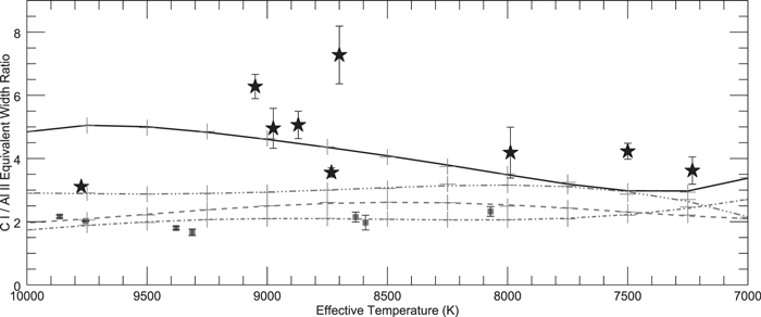
Figure 4. C i 1657 Å /Al ii 1671 Å equivalent width ratio of Lambda Boo stars, normal stars, and four sets of model spectra. Star icons are observed Lambda Boo ratios, and filled squares indicate normal star ratios. For the models, the solid line indicates the model derived using "Heiter's mean" Lambda Boo abundance pattern (see Section 3.4 for details), the dashed–dotted–dotted–dotted line indicates [M/H] = −2.00 models, the long dashed line indicates [M/H] = −1.00 models, and the dashed–dotted line indicates solar [M/H] = 0.00 models. Measurement uncertainty is given for each star, but was not included for the "noise-free" models (indicated by "+" signs). There is good agreement between both the observed Lambda Boo (filled stars) and normal star (filled squares) measurements with their respective models. Note that not all Lambda Boo stars line up with the "Heiter's mean" model with [M/H] = −1.00, because their [M/H] values range from −0.58 to −2.03 (see individual [M/H] and/or [Fe/H] values provided in Table 1). For example, HD 170680 (Teff = 9774 K) and HD 221756 (Teff = 8733 K) have C i/Al ii ratios lower than the mean Lambda Boo model ratio, but can nonetheless be confirmed as Lambda Boo stars. Both of these stars have [M/H] values greater than the Lambda Boo average of −1.00 (−0.50 and −0.75 respectively), but have C, N, O, and S values near solar. Their measurements reflect their peculiar abundance pattern. Despite having a ratio lower than that of our "average" Lambda Boo models, their ratios are significantly higher than the corresponding metal-poor models with the same general parameters (e.g., Teff and [M/H]).
Download figure:
Standard image High-resolution imageAlthough both C i 1657 Å and C i 1931 Å lines were observed with IUE's SWP camera (1145–1975 Å), the data quality longward of 1900 Å is generally very poor. Since both the C i 1657 Å and Al ii 1671 Å features are blended lines (Table 4), it is very important to make sure that the equivalent width measurements are inclusive of all of the necessary lines, regardless of any rotational broadening effects, and that this is repeatable for all measurements (see Section 2.5). For a typical Lambda Boo star, the C i 1657 Å blend is very strong and the Al ii 1671 Å blend is relatively weak, so the accuracy of the C i 1657 Å/Al ii 1671 Å line ratio heavily depends on the accuracy of the equivalent width measurement of Al ii 1671 Å.
We also measured the C i 1657 Å/Al ii 1671 Å equivalent width ratios of a group of normal (standard) stars with different effective temperatures. Since late A-type stars and early F-type stars do not have much flux shortward of 1700 Å, it is hard to find standard (normal) stars cooler than A7 V (∼7920 K) with existing IUE SWP high data. To help alleviate this problem, we generated a set of synthetic models for normal stars ([M/H] = 0.00) with effective temperatures ranging from Teff = 6000 to 11,000 K in steps of 250 K. Figure 4 clearly shows a good general agreement between the observed normal stars and the synthetic models for normal stars (Table 2). It also illustrates how accurately the equivalent width ratio must be determined in order to discriminate between Lambda Boo stars and other metal-poor stars. For example, around 9500 K the error bars can be large, whereas below 8000 K a large error bar could lead to a mis-classification if the measured ratio is close to the Heiter mean (solid line in Figure 4).
In the past, some stars have been (mis)classified as Lambda Boo-type based on their metal weakness alone. In order to show that the C i/Al ii ratio is capable of separating Lambda Boo stars from other metal-poor stars, we generated a set of synthetic models for "normal" metal-poor stars. Between 7500 and 10,000 K, the C i/Al ii equivalent width ratios of Lambda Boo stars are very different from the C i/Al ii ratios of metal-poor models. We also compared the C i/Al ii equivalent width ratios of Lambda Boo stars with Heiter's "mean" Lambda Boo star models discussed in Section 3.4. Our nine Lambda Boo stars do not match with the "mean" Lambda Boo star models (with [M/H] = −1.00) exactly, because they have [M/H] ranging from −0.58 to −2.00 (Table 1). The stellar parameters of individual stars (log g, vturb, etc.) also vary slightly from our model values of log g = 4.00 and vturb = 2.0 km s−1. Figure 4 clearly shows the Lambda Boo stars' C i 1657 Å/Al ii 1671 Å equivalent width ratio is a function of both the star's effective temperature and metallicity. One cannot use a single C i/Al ii cut-off value as a Lambda Boo classification criterion, but with the models we generated with various effective temperatures and metallicities, we can specify the C i/Al ii cut-off value for a specific star based on its effective temperature and metallicity. For all effective temperatures in the range of 7300–10,000 K, a C i/Al ii ratio >3 is a firm indication that the star is a Lambda Boo. For stars with a ratio between 2 and 3, it is important to first determine the metallicity and effective temperature to see if the ratio falls above the expected value. Stars with solar abundances all have ratios  . For example, there are two Lambda Boo stars in Figure 4 with ratios well below the "Heiter's mean" (which is based on [M/H] = −1.0; solid line) but nevertheless well above the value expected for their lower metallicities.
4.3. Is the "1600 Å" Depression a Defining Characteristic of Lambda Boo Stars?
Baschek et al. (1984) use low and high resolution IUE-spectra to distinguish Lambda Boo stars from normal stars. The strong depression at 1600 Å (Figure 5) is one of the main criteria they used to identify Lambda Boötis stars. However, the 1600 Å depression has also been detected in field horizontal branch stars and cool DA white dwarfs (Jaschek et al. 1985).

Figure 5. Histogram is Lambda Boo's IUE spectrum SWP17873, which shows a ∼120 Å wide "depression" centered around 1600 Å. We show 3 model spectra for comparison: the solid black line represents a model of the "Heiter mean" Lambda Boo star (see Section 3.4), the dashed–dotted–dotted–dotted line represents a metal-poor star with [M/H] = −2.00, and the dashed–dotted line represents a "normal" star with [M/H] = 0.00. All models were generated with an effective temperature of 8700 K and have been convolved to the resolution of IUE low-dispersion spectra. This figure illustrates that both metal-poor stars and Lambda Boo stars can exhibit this depresssion, but it is absent in normal stars. Shortward of 1600 Å, both Lambda Boo and metal-poor stars show significantly more continuum flux than the normal stars. Shortward of 1550 Å, they diverge, with the mean Lambda Boo spectrum appearing mid-way between normal and metal-poor stars.
Download figure:
Standard image High-resolution imageOur goal is not to determine the cause of this so-called "1600 Å" depression (Holweger et al. 1994), but rather to assess its use as a Lambda Boo classification criterion. Using model spectra we show in Figure 6 that all metal-poor stars with effective temperature of 8000–9000 K and log g near 4.0 also have a detectable 1600 Å depression. Therefore, a detectable 1600 Å depression is not a unique Lambda Boo classification criterion.
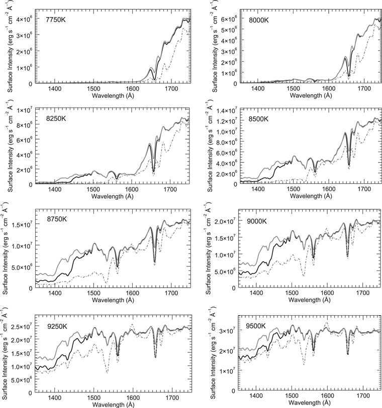
Figure 6. By comparing three models with different elemental abundances we conclude that the 1600 Å depression is visible only over a limited temperature range in both Lambda Boo stars and metal-poor stars. The top spectrum (gray line) is the model of metal-poor stars with [M/H] = −1.00, the middle spectrum (black line) is the model of "mean" Lambda Boo stars with [M/H] = −1.00, and the bottom spectrum (dashed–dotted line) is the model of "normal" stars with [M/H] = 0.00. All synthetic spectra have been convolved to the resolution of IUE low-dispersion spectra.
Download figure:
Standard image High-resolution imageFigures 5 and 6 show that the UV excess continuum in metal-poor and Lambda Boo spectra shortward of 1550 Å makes the apparent depression centered at 1600 Å more clearly visible. This blanketing effect is highly dependent on the metallicity; the lower the [M/H], the higher the general flux level in the ultraviolet, but it is the other way around in the visible/IR region (Figure 7). Shortward of 1550 Å, there is a significant difference between metal-poor and Lambda Boo stars. The latter have higher C, N, O, and S abundances, so in this spectral region the Lambda Boo stars are fainter due to the higher C i continuous opacity and higher carbon line opacity. This provides another constraint, in addition to the C i/Al ii equivalent width ratio, to discriminate between Lambda Boo stars and other metal-poor stars in the ultraviolet.
Figure 7. Comparison of two models with different elemental abundances shows the UV excess shortward of 1550 Å is a result of the metallic-line blanketing effect. The black line spectrum is the model of "mean" Lambda Boo stars (see Section 3.4 for details) and the dashed–dotted line spectrum is the model of "normal" stars with [M/H] = 0.0. All synthetic spectra have been convolved to the resolution of IUE low-dispersion spectra.
Download figure:
Standard image High-resolution imageWe inspected IUE low-dispersion spectra of 27 Lambda Boo stars and found that only 8 of them show the 1600 Å depression (Table 6). We found that not all Lambda Boo stars have detectable 1600 Å depressions and that the presence of a depression is not enough to discern a Lambda Boo star from other metal-poor stars.
Table 6. Lambda Boo Stars That Show 1600 Å Depression
| Identification | Mean Teff | Spectral Type | [M/H] |
|---|---|---|---|
| (K) | (SIMBAD) | ||
| HD 183324 | 9050 | A0 V | −1.80 |
| HD 110411 | 8975 | A3 Va | −1.00 |
| HD 31295 | 8871 | A3 Va | −1.24 |
| HD 221756 | 8733 | A1 Va | −0.75 |
| HD 125162 | 8700 | A3 Va | −2.00 |
| HD 192640 | 7988 | A2 V | −2.00 |
| HD 11413 | 7956 | A1 V | −2.03 |
| HD 111786 | 7500 | A0 III | −0.58 |
Download table as: ASCIITypeset image
4.4. Weak Mg ii Line is a Signature of All Metal-poor A/F Stars
Ohanesyan (2008) demonstrates that peculiar A-type stars—including Lambda Boo stars—can be identified by analyzing the equivalent width of the 2786–2810 Å Mg ii h+k spectral band as a function of the star's Teff. We measured the equivalent width of the 2794.1–2805.3 Å spectral band of 20 Lambda Boo stars with suitable IUE spectra, as well as all of our model spectra. We chose a slightly narrower band than Ohanesyan (2008) because we only want to measure the total equivalent width of Mg ii k (2796.4 Å in vacuum) and h (2803.5 Å in vacuum) resonance lines (Table 4). The observed spectra have a small amount of additional absorption due to interstellar, and possibly circumstellar material, which is not included in the synthetic spectra (Figure 8). For rapidly rotating stars with high resolution spectra, it is possible to remove the contribution to the overall equivalent width from this narrow component. Because it is not possible to do this in all the spectra, and because its contribution to the overall equivalent width in this 11 Å bandpass is small, we did not attempt to make any corrections to the values shown in Figure 9.
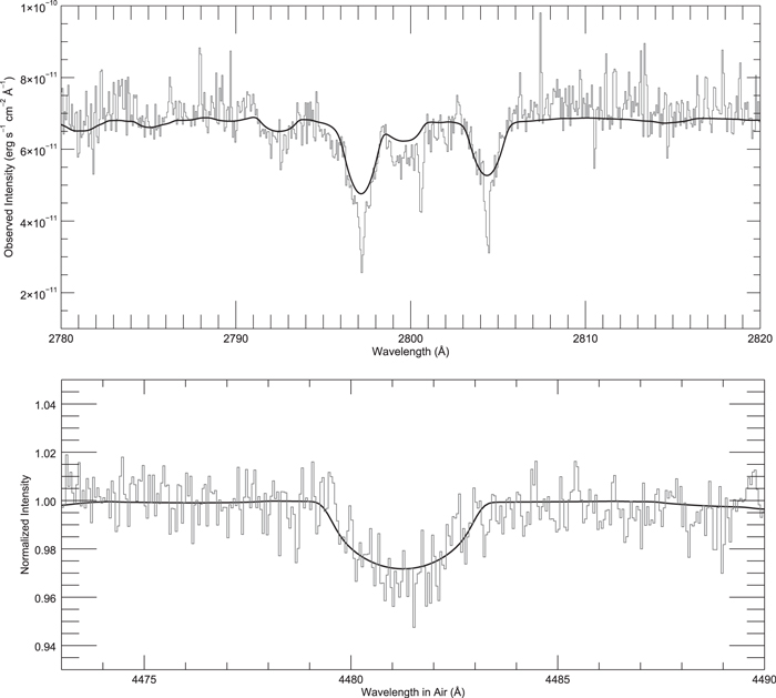
Figure 8. Top panel shows the observed IUE spectrum (gray histogram) of Lambda Boo (v sin i = 123 km s−1) in the wavelength region of the Mg ii 2800 Å doublet. It can be fit well by a single-temperature synthetic spectrum (solid black line), except for the additional interstellar absorption, which is not included in the synthetic spectrum. The bottom panel shows that the observed ELODIE spectrum of Lambda Boo in the wavelength region of the Mg ii 4481 Å blended feature can also be fit well by the same single-temperature synthetic spectrum we used to fit the IUE spectrum. The synthetic spectrum has been rotationally broadened and convolved to the resolution of the observed spectra.
Download figure:
Standard image High-resolution image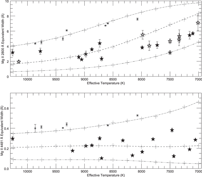
Figure 9. We compared the Mg ii 2800 Å (top panel) and Mg ii 4481 Å (bottom panel) equivalent widths (as a function of Teff and [M/H]) and measured for three sets of models, observed Lambda Boo stars, and observed normal stars. Filled and empty star icons designate observed Lambda Boo equivalent widths measured using high- and low-dispersion IUE data, respectively. Filled squares indicate normal star equivalent widths, and "+" signs indicate our equivalent measurements of the models. Measured error is given per star, but was not included for the models since their error is not significant. For the models, the dashed–dotted–dotted–dotted line indicates [M/H] = −2.00 model equivalent widths, the long dashed line indicates [M/H] = −1.00 model equivalent widths and the dashed–dotted line indicates solar [M/H] = 0.00 model equivalent widths. The "model" lines have been calculated using a 5th degree polynomial fit of our model measurements. There is good agreement between both the observed Lambda Boo and normal star measurements with their respective models (see Table 1 for Lambda Boo stars' [M/H] values).
Download figure:
Standard image High-resolution imageFor those Lambda Boo stars with existing ELODIE data, we also measured the equivalent width of Mg ii 4481 Å (Figure 8) and compared them with three sets of models (the [M/H] = −2.00 models, the [M/H] = −1.00 models, and the solar [M/H] = 0.00 models). All the synthetic spectra were convolved to the resolution of the ELODIE spectra (R = 42,000). Figure 9 clearly shows that the equivalent width of Mg ii 4481 Å is accurately predicted by our models, and it is a function of both the star's Teff and [M/H], and one cannot use the weak Mg ii 4481 Å line alone to distinguish Lambda Boo stars from other metal-poor stars. Furthermore, the temperature dependence of the Mg ii 4481 Å equivalent width mimics that of the 2800 Å Mg ii feature. Another widely accepted visible characteristic of Lambda Boo stars is that "the ratio Mg ii 4481 Å/Fe i 4383 Å is significantly smaller than in normal A-type stars" (Gray & Corbally 2009). However, the weaker Mg ii 4481 Å/Fe i 4383 Å equivalent width ratio was judged by eye using classification-resolution spectra, which could include blends with many other lines. We have measured the equivalent widths of the blended 4383 Å feature in both our grid of models and the higher-resolution ELODIE spectra. The Fe i 4383 Å line is very weak, especially for hotter stars. Even in the noise-free models it is hard to measure the ratio for effective temperatures greater than 9500 K. For stars with v sin i >80 km s−1, rotational broadening makes it more difficult to measure the lines' equivalent width, so the measurement error is large. We have, however, demonstrated that a weak 4481 Å line is a good indicator that a star is metal-poor.
4.5. Do Beta Pictoris and Vega Satisfy the UV Classification Criteria for Lambda Boo Stars?
The Lambda Boo class has recently regained the spotlight because of the discovery of giant planets around the Lambda Boo star HR 8799 (Gray & Kaye 1999; Marois et al. 2008) and around a "suggested" Lambda Boo star Beta Pictoris (Bonnefoy et al. 2011). The discovery of a giant asteroid belt around Vega, another suggested Lambda Boo star, also raises the possibility that it could have hidden planets (Su et al. 2013). Thus, there could be a link between Lambda Boo stars and planet-bearing stars (Jura 2015). We would like to investigate whether HR 8799, Vega, and Beta Pictoris satisfy the UV criteria we established in this study. Unfortunately, there are no existing UV data for HR 8799, but we have applied the UV criteria established in this paper to Beta Pictoris and Vega.
Beta Pictoris is the original and best-known example of a star surrounded by a dusty debris disk, and it has ample existing IUE data. King & Patten (1992) claim that "Beta Pic seems to meet most criteria required for a Lambda Boo classification." On the other hand, Holweger & Rentzsch-Holm (1995) conclude that "Beta Pic most probably is a superficially normal A star with solar metallicity." Gray et al. (2006) observed Beta Pic using CTIO 1.5 m telescope with the Cassegrain spectrograph and the Loral 1200 X 800 CCD (with a 2 pixel resolution of 2.6 Å in the spectral range of 3800–5150 Å). They conclude that Beta Pictoris has a spectral type of A6 V with no peculiarities detected.
We examined all of Beta Pic's existing archival IUE data. We conclude that Beta Pic is not a Lambda Boo star because:
- 1.
- 2.the 1600 Å depression of a metal-deficient A-type star with Teff = 8182 K and Beta Pic's stellar parameters should be clearly visible, but we did not detect one;
- 3.its Mg ii equivalent widths are the same as normal A-type stars with Beta Pic's Teff (Figure 10);
- 4.Beta Pic's abundance pattern is like those of normal stars with solar abundances (Holweger & Rentzsch-Holm 1995).

Figure 10. In all panels, Beta Pic and Vega's measurements are designated with a diamond and a triangle, respectively. The solid line indicates the "Heiter's mean" Lambda Boo model (see Section 3.4 for details), the dashed–dotted line indicates solar [M/H] = 0.00 models and the dotted line indicates [M/H] = −0.50 models. These three lines are 5th degree polynomial fits of the model measurements, which are given as "+" symbols. Filled and empty star icons designate observed Lambda Boo equivalent widths measured using high and low-dispersion IUE data, respectively. The left panel shows that the C i 1657 Å/Al ii 1671 Å ratio of Beta Pic and Vega are near the [M/H] = 0.00 and [M/H] = −0.50 models respectively. The middle panel shows that Beta Pic's Mg ii 2800 Å equivalent width is the same as normal A-type stars with Beta Pic's Teff and an [M/H] value of near zero. Vega's Mg ii 2800 Å equivalent width is in line with a metal-poor A-type star with [M/H] = −0.50 and Vega's Teff. The right panel shows that both Beta Pic and Vega's Mg ii 4481 Å equivalent widths are separate from Lambda Boo stars with the same Teff. It should be noted that the Mg ii 4481 Å equivalent width alone cannot be used as a conclusive diagnostic for the Lambda Boo class.
Download figure:
Standard image High-resolution image
Table 7. Data Used for Evaluating the Lambda Boo Status of Beta Pictoris and Vega
| Identification | Mean Teff | Teff Differencea | [M/H] | IUE SWP | IUE LWP/LWR | Visible Observation |
|---|---|---|---|---|---|---|
| (K) | (K) | (.mxhi) | (.mxhi) | |||
| Beta Pictoris | 8182 (1), (2), (3), (4) | −54/+18 | 0.05 (10), 0.09 (11) | 49200 | 27086 | CTIO datab |
| (HD 39060) | ||||||
| Vega | 9562 (5), (6), (7), (8), (9) | −62/+88 | −0.43 (10), −0.50 (7) | 32870 | 04837 | 20041109/0009 (ELODIE dataset/imnum) |
| (HD 172167) | 20041105/0016 (ELODIE dataset/imnum) | |||||
| 20040326/0062 (ELODIE dataset/imnum) | ||||||
| 20000617/0008 (ELODIE dataset/imnum) | ||||||
| 20040831/0017 (ELODIE dataset/imnum) |
Notes.
aThe difference between the mean effective temperature and the lowest/highest effective temperature. bTaken with the 1.5 m telescope using the Cassegrain spectrograph.References. (1) Holweger et al. (1997), (2) Lanz et al. (1995), (3) Hubrig et al. (2009), (4) Heap et al. (1994), (5) Dreiling & Bell (1980), (6) Hill & Landstreet (1993), (7) Fitzpatrick (2010), (8) Castelli & Kurucz (1993), (9) Lane & Lester (1984), (10) Gray et al. (2003), (11) Ohanesyan (2008).
Download table as: ASCIITypeset image
Vega was first noted to have Lambda Boo-like abundances by Baschek & Slettebak (1988). Since then there has been a long debate on whether Vega should be considered as a member of the Lambda Boo class. Ilijic et al. (1998) performed an elemental abundance analysis using a high-dispersion spectrum in the visible region, and they suggest that Vega is a "mild" Lambda Boo star based on its mild metal under-abundance. Although Vega does have an abundance pattern like those of mild Lambda Boo stars, with C and O near solar and metals being about 0.5 dex below solar (see Ilijic et al. 1998; Figure 7 of Hekker et al. 2009; Fitzpatrick 2010), it does not have any of Lambda Boo's UV characteristics. We conclude that Vega is not a Lambda Boo star because:
- 1.it has a C i 1657 Å/Al ii 1671 Å equivalent width ratio that is too low for a Lambda Boo star with the same effective temperature as Vega (Figure 10);
- 2.it does not have a 1600 Å depression though for a star with Teff = 9562 K one should be clearly visible;
- 3.both its C i 1657 Å/Al ii 1671 Å equivalent width ratio and its Mg ii 2800 Å equivalent width are similar to normal A-type stars with the same Teff and [M/H] (−0.50 dex) (Figure 10);
- 4.its Mg ii 4481 Å equivalent width is slightly above our predicted value for normal A type stars with the same Teff and [M/H]. It should be noted that the Mg ii 4481 Å equivalent width is not a conclusive diagnostic for the Lambda Boo class. We are currently working on a visible classification criteria that can differentiate Lambda Boo stars from other metal-poor stars in a manner similar to what we have done in this paper.
5. CONCLUSIONS
In this paper, we studied 38 Lambda Boo stars with existing IUE and/or ELODIE data. We also analyzed 120 model spectra of normal stars, metal-poor stars, and "mean" Lambda Boo stars. We found that:
- 1.Lambda Boo stars' IUE spectra can be reproduced quite well with single-temperature LTE synthetic spectra. Lambda Boo indeed has extreme deficiencies of iron peak elements, but its C, N, O, and S are near solar. We have also confirmed that its aluminum abundance is 0.50 dex more depleted than iron (Heiter 2002).
- 2.The UV criteria cited in the literature to classify Lambda Boo stars should be both Teff and [M/H] dependent.
- 3.The 1600 Å depression cannot serve as a standalone Lambda Boo classification criterion.
- 4.We cannot use the total equivalent width of either the Mg ii 2800 Å blend or the Mg ii 4481 Å line to distinguish between Lambda Boo stars and other metal-poor stars.
- 5.The C i 1657 Å/Al ii 1671 Å equivalent width ratio is the best single UV criterion to distinguish between Lambda Boo stars and metal weak stars. This ratio is a function of the individual star's effective temperature and [M/H]. Between 7500 and 10,000 K, the C i/Al ii equivalent width ratios of Lambda Boo stars are very different from the C i/Al ii ratios of models of metal-poor stars.
- 6.Beta Pictoris and Vega should not be classified as Lambda Boo stars based on the criteria we established in this study.
- 7.We need new classification criteria for cooler (F-type) Lambda Boo candidates. We cannot use the C i 1657 Å/Al ii 1671 Å equivalent width ratio as a classification criterion because these stars do not have enough flux shortward of 1700 Å.
Our future work will include:
- 1.obtaining UV spectra of HR 8799 using the HST in order to confirm its Lambda Boo status;
- 2.utilizing synthetic visible spectra to explore the physical basis for the classification of Lambda Boo Stars;
- 3.compiling a list of bona fide Lambda Boo stars that pass our quantitative UV and visible classification criteria;
- 4.using Herschel and Spitzer data to compile a list of bona fide Lambda Boo stars with circumstellar disks for exploring the possible link between Lambda Boo stars and planet-bearing stars.
This program is supported by grants from the National Science Foundation to California State University Fullerton (AST-1211213), the College of Charleston (AST-1211221, AST-1109695), and Appalachian State University (AST-1211215). Some of the data presented in this paper were obtained from the Mikulski Archive for Space Telescopes (MAST). STScI is operated by the Association of Universities for Research in Astronomy, Inc., under NASA contract NAS5-26555. Support for MAST for non-HST data is provided by the NASA Office of Space Science via grant NNX13AC07G and by other grants and contracts. This research has made use of the SIMBAD database, operated at CDS, Strasbourg, France. This research has also made use of the VizieR catalog access tool, CDS, Strasbourg, France.
Footnotes
- 6
The "IUE Ultraviolet Spectral Atlas of Standard Stars" can be accessed at https://archive.stsci.edu/prepds/iuesass_web/iue.html.
- 7
MK standards can be found at http://www.pas.rochester.edu/~emamajek/spt/.
- 8
MAST data can be found at https://archive.stsci.edu/iue/.
- 9
The original "feature.pro" program, as well as the rest of the IUEDAC library, can be found at https://archive.stsci.edu/iue/prolog.html.
- 10
SPECTRUM can be downloaded from http://www.appstate.edu/~grayro/spectrum/spectrum.html.
- 11
Castelli and Kurucz's ATLAS9 program and LTE atmosphere models can be accessed from http://www.oact.inaf.it/castelli.
- 12
Gray's manual for SPECTRUM can be accessed at http://www.appstate.edu/~grayro/spectrum/spectrum276.pdf.
- 13
The Castelli and Kurucz's LTE atmosphere models can be accessed from http://www.oact.inaf.it/castelli/castelli/grids.html.