


ABSTRACT
The second realization of the International Celestial Reference Frame (ICRF2), which is the current fundamental celestial reference frame adopted by the International Astronomical Union, is based on Very Long Baseline Interferometry (VLBI) data at radio frequencies in X band and S band. The European Space Agency's Gaia mission, launched on 2013 December 19, started routine scientific operations in 2014 July. By scanning the whole sky, it is expected to observe ∼500,000 Quasi Stellar Objects in the optical domain an average of 70 times each during the five years of the mission. This means that, in the future, two extragalactic celestial reference frames, at two different frequency domains, will coexist. It will thus be important to align them very accurately. In 2012, the Laboratoire d'Astrophysique de Bordeaux (LAB) selected 195 sources from ICRF2 that will be observed by Gaia and should be suitable for aligning the radio and optical frames: they are called ICRF2-Gaia transfer sources. The LAB submitted a proposal to the International VLBI Service (IVS) to regularly observe these ICRF2-Gaia transfer sources at the same rate as Gaia observes them in the optical realm, e.g., roughly once a month. We describe our successful effort to implement such a program and report on the results. Most observations of the ICRF2-Gaia transfer sources now occur automatically as part of the IVS source monitoring program, while a subset of 37 sources requires special attention. Beginning in 2013, we scheduled 25 VLBI sessions devoted in whole or in part to measuring these 37 sources. Of the 195 sources, all but one have been successfully observed in the 12 months prior to 2015 September 01. Of the sources, 87 met their observing target of 12 successful sessions per year. The position uncertainties of all of the ICRF2-Gaia transfer sources have improved since the start of this observing program. For a subset of 24 sources whose positions were very poorly known, the uncertainty has decreased, on average, by a factor of four. This observing program is successful because the two main goals were reached for most of the 195 ICRF2-Gaia transfer sources: observing at the requested target of 12 successful sessions per year and improving the position uncertainties to better than 200 μas for both R.A. and decl. However, scheduling some of the transfer sources remains a challenge because of network geometry and the weakness of the sources, and this will be one focus of future sessions used in this ongoing program.
Export citation and abstract BibTeX RIS
1. INTRODUCTION
The second realization of the International Celestial Reference Frame (ICRF), named ICRF2 is the current radio catalog, which contains accurate celestial positions of 3414 compact radio sources (extragalactic radio sources and quasars), as measured by Very Long Baseline Interferometry (VLBI; Schuh & Behrend 2012). The underlying accuracy of ICRF2 is 40 μas (Fey et al. 2009, 2015).
On 2013 December 19, the spacecraft of the ESA's Gaia mission was launched from French Guyana. After a seven-month commissioning phase, the mission entered into its operational phase in 2014 July. The mission's primary scientific product will be an optical catalog with the positions, motions, brightnesses, and colors of the surveyed objects. The first intermediate catalog will be released mid-2016 and the final version is expected by 2021 (see http://sci.esa.int/gaia/). The position accuracy anticipated after the commissioning phase is of the order of 20 μas at a magnitude of 15, 100 μas at a magnitude of 18, and 400 μas at a magnitude of 20 (F. Mignard 2014, private communication).
Gaia will survey the whole sky, including observing the extragalactic sources used for the celestial reference frame: the Quasi Stellar Objects. The Gaia Celestial Reference Frame (GCRF) in the optical domain should be aligned with the ICRF2 in the radio domain, ensuring the consistency of the fundamental frame in the future. This alignment will be done based on a set of common quasars among the ∼500,000 quasars that Gaia is expected to observe. Aligning the two frames will permit many advances in science from a better understanding of the AGN physics to the quantification of the shifts between radio and optical positions (Kovalev et al. 2008).
In this paper, we describe the International VLBI Service for Geodesy and Astrometry (IVS) efforts made to regularly observe 195 ICRF2 sources that should align the ICRF and the GCRF. The IVS is an international collaboration of organizations, that operate and support VLBI components. The objectives of IVS are to provide a service to support geodetic, geophysical, and astrometric research and operational activities. The service promotes research and development activities in all aspects of the geodetic and astrometric VLBI techniques. It fosters interaction with the community of users of VLBI products and supports the integration of VLBI into a global Earth observing system4 (Behrend 2013).
Section 2 describes the selection of these 195 sources, as well as the IVS monitoring program in which we included these sources and the set of sources that we schedule in specific sessions. We report on the scheduling strategy in Section 3. In Section 4, we present the improvements in observation frequency, source position accuracy, and flux information. We discuss how the station observing network could be developed to have the sensitivity to observe the entire set of 195 sources in Section 5.
2. CANDIDATE SOURCES TO ALIGN THE VLBI AND GAIA FRAMES
2.1. Selection of 195 ICRF2-Gaia Transfer Sources
The Laboratoire d'Astrophysique de Bordeaux (LAB) developed a strategy, explained in detail in Bourda et al. (2008), to select candidate sources for aligning the GCRF and the ICRF. The selected sources (1) are both contained in the ICRF and the Véron-Cetty & Véron (2006) optical catalog, (2) have an optical counterpart brighter than the apparent magnitude V = 18, and (3) have high astrometric quality, e.g., an acceptable observed structure as defined by the Structure Index introduced in Fey & Charlot (1997). The LAB identified 70 sources as good candidates when applying their criteria to the ICRF-Ext2 catalog. This catalog is the second extension of the first ICRF (Fey et al. 2004). It contains 717 sources, 109 more sources than are contained in the original ICRF.
Because the number of these candidate sources is low, the LAB extended its study to weak radio sources of the NRAO VLA Sky Survey (NVSS) catalog5
(Condon et al. 1998). The LAB extracted 447 sources with the following characteristics: they are not ICRF or VCS sources (sources in the VLBA Calibrator Survey6
; Beasley et al. 2002; Fomalont et al. 2003; Petrov et al. 2005, 2006, 2008; Kovalev et al. 2007), their optical magnitude is less than or equal to 18, their total flux density from NVSS is greater than 0.02 Jy and their decl. are above  . Specific VLBI observing programs were designed with the European VLBI Network and the VLBA to observe these sources. The first campaign of observations was for detection (Bourda et al. 2010), the second campaign for imaging (Bourda et al. 2011), and the third campaign for accurate astrometry of the most compact sources, where 119 suitable sources were successfully observed (Bourda et al. 2015).
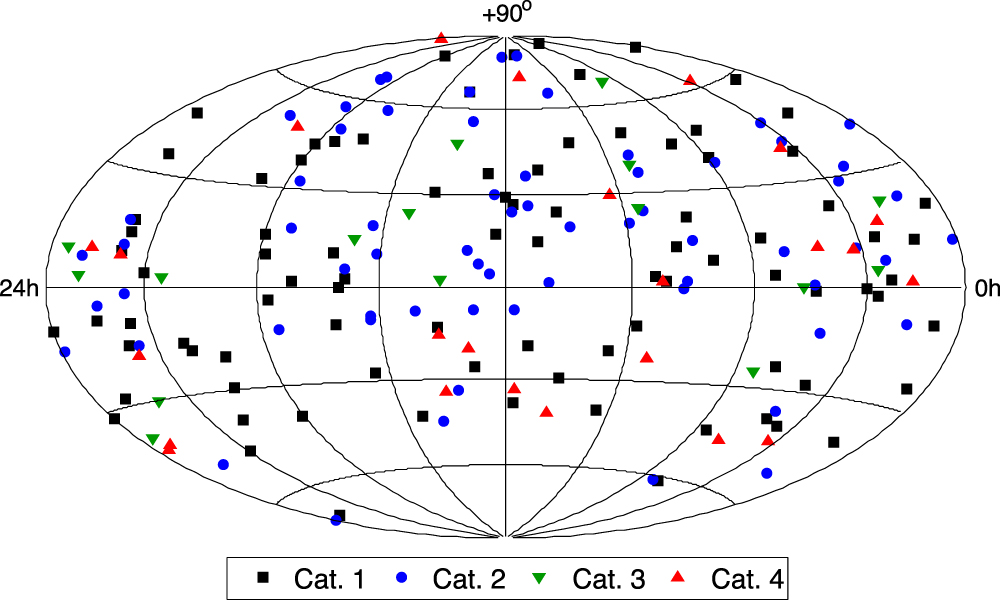
In parallel, in 2012, the LAB submitted a proposal to the IVS (see Bourda & Charlot 2012) to observe 195 ICRF2 transfer sources in the context of the Gaia mission. These 195 sources were selected within the ICRF2 catalog the same way the 70 sources were selected from the ICRF-Ext2, i.e., for their optical magnitude and astrometric suitability (Charlot et al. 2013; Bourda et al. 2015). These sources are called ICRF2-Gaia transfer sources. To get an observation frequency comparable to that of the Gaia mission, which is scheduled to observe sources an average of 70 times each during the five years of the mission, the LAB requested most of the ICRF2-Gaia transfer sources to be observed at least once per month if possible. The LAB set an initial threshold of 200 μas for positional accuracy. This subjective threshold was selected as a reasonable value given the overall accuracy of the sources observed in the IVS monitoring program because the principal goal was to improve the position of the poorly observed ICRF2-Gaia transfer sources. Based on the Goddard VLBI global solution 2012a7 and the source list of the IVS source monitoring program at the time, the 195 sources were divided into four different categories.
- 1.Category 1 (89 sources): sources in the IVS source monitoring program that were sufficiently observed.
- 2.Category 2 (66 sources): sources in the IVS source monitoring program that were not sufficiently observed.
- 3.Category 3 (16 sources): sources not in the IVS source monitoring program but with a sufficient position accuracy.
- 4.Category 4 (24 sources): sources not in the IVS source monitoring program and with poor position accuracy.
As seen in Figure 1, the 195 ICRF2-Gaia transfer sources are well distributed, except for the band  ,
, ![$-90^\circ {\rm{]}}$](https://content.cld.iop.org/journals/1538-3881/151/3/79/revision1/aj522672ieqn3.gif) that contains only four sources.
that contains only four sources.

Figure 1. 195 ICRF2-Gaia transfer sources determined by the LAB.
Download figure:
Standard image High-resolution imageTable 1 lists the 195 ICRF2-Gaia transfer sources, along with their coordinates from the latest GSFC catalog (2015a) and most recent flux values from the sked flux catalog8 (status: 2015 August 28) and from the Bordeaux VLBI Image Database9 (BVID; Collioud & Charlot 2009; status: 2015 September 11). The fluxes are computed from data available through 2015 August 27 for the sked catalog and through 2013 July 24 for BVID (see Section 4.3).
Table 1. Candidate ICRF2-Gaia Transfer Sources to Align the Radio Catalog and the Gaia Catalog
| Source Name | J2000.0 Coordinates in 2015a GSFC Cataloga | GSFC Fluxb (sked) | BVID Fluxb | Initial | ||||||||||||
|---|---|---|---|---|---|---|---|---|---|---|---|---|---|---|---|---|
| R.A. α | Decl. δ | Formal Errors | Sess. | Obs. | X Band | S Band | X Band | S Band | Gaia | |||||||
| IVS | IAU/J2000 | h | m | s | ° | ' | " |

|

|
# | # | cat. | ||||
| 0016+731 | J0019+7327 | 00 | 19 | 45.7863648 | +73 | 27 | 30.0175664 | 8 | 2 | 734 | 83780 | 4.28 | 0.73 | 0.90 | 0.67 | 1 |
| 0025+197 | J0028+2000 | 00 | 28 | 29.8184839 | +20 | 00 | 26.7439348 | 17 | 22 | 78 | 2615 | 0.25 | 0.16 | 0.19 | 0.17 | 1 |
| 0035–252 | J0038–2459 | 00 | 38 | 14.7355028 | –24 | 59 | 02.2352821 | 18 | 21 | 140 | 2696 | 0.23 | 0.18 | 0.65 | 0.40 | 1 |
| 0048–097 | J0050–0929 | 00 | 50 | 41.3173869 | –09 | 29 | 05.2103565 | 4 | 6 | 2016 | 45436 | 0.62 | 0.20 | 0.55 | 0.52 | 1 |
| 0059+581 | J0102+5824 | 01 | 02 | 45.7623787 | +58 | 24 | 11.1365770 | 2 | 2 | 2491 | 361024 | 3.36 | 2.49 | 1.69 | 1.91 | 1 |
| 0104–408 | J0106–4034 | 01 | 06 | 45.1079685 | −40 | 34 | 19.9603641 | 9 | 9 | 1662 | 17435 | 1.28 | 3.52 | 0.76 | 0.64 | 1 |
| 0119+115 | J0121+1149 | 01 | 21 | 41.5950426 | +11 | 49 | 50.4131761 | 3 | 6 | 1507 | 54260 | 1.81 | 2.34 | 1.55 | 1.80 | 1 |
| 0133+476 | J0136+4751 | 01 | 36 | 58.5948052 | +47 | 51 | 29.1000322 | 2 | 2 | 1860 | 184101 | 1.70 | 0.96 | 3.87 | 1.04 | 1 |
| 0215+015 | J0217+0144 | 02 | 17 | 48.9547539 | +01 | 44 | 49.6990157 | 6 | 7 | 216 | 15613 | 0.44 | 0.35 | 0.73 | 1.00 | 1 |
| 0229+131 | J0231+1322 | 02 | 31 | 45.8940565 | +13 | 22 | 54.7162577 | 3 | 5 | 2867 | 86610 | 1.93 | 3.38 | 2.15 | 1.74 | 1 |
Notes. The formal errors in the table come directly from the GSFC solution and are likely too optimistic. A more realistic estimate would be obtained by applying a scale factor of 1.5 to the formal uncertainties followed by a root-sum-square increase of 40 μas of error in quadrature to the quoted values. This was the procedure adopted for ICRF2 (Fey et al. 2009, 2015). Table 1 is published in its entirety in the electronic edition of the Astrophysical Journal. A portion is shown here for guidance regarding its form and content.
aThe coordinates are from the latest version of the GSFC solution 2015a in IERS format (status: 01 September 1 2015). Units of R.A. α are hours, minutes, and seconds; units of decl. δ are degrees, minutes, and seconds; units of uncertainties ( and
and  ) are in μas. The uncertainties for α are not corrected from
  .
bThe flux values are from sked (status: 2015 August 28) and BVID (status: 2015 September 11). Units are Jy.
.
bThe flux values are from sked (status: 2015 August 28) and BVID (status: 2015 September 11). Units are Jy.
Only a portion of this table is shown here to demonstrate its form and content. A machine-readable version of the full table is available.
Download table as: DataTypeset image
2.2. Inclusion in the IVS Source Monitoring Program
Beginning in 2003 June, the Goddard VLBI group developed a program to purposefully monitor when sources were observed and to increase the observations of "under-observed" sources. The heart of the program consists of a MySQL database that on a session-by-session basis keeps track of the number of observations that are successfully correlated and the number of observations that are used in a session. In addition, there is a MySQL table in the database that contains the target number of successful sessions over the last 12 months. Initially, this table only contained two categories. Sources in the geodetic catalog had a target of 12 sessions/year; the remaining ICRF-1 defining sources had a target of two sessions/year. All other sources did not have a specific target. As the program evolved, different kinds of sources with different observing targets were added. During the scheduling process, the scheduler has the option of automatically selecting sources that have not met their target (Gipson et al. 2014). Currently, the IVS weekly R1 and R4 sessions as well as the bi-monthly RDV sessions participate in this program. Each of these sessions includes up to 10 "monitoring" sources.
In 2013 March, we added all 195 ICRF2-Gaia transfer sources to the IVS source monitoring program with an observation target of 12 successful sessions per year.
2.3. Focus on a Specific Set of Sources
Because of the network geometry and/or their low flux (flux values lower than 0.10 Jy), some of the 195 ICRF2-Gaia transfer sources were not automatically scheduled in the IVS source monitoring program. We decided to schedule them manually in dedicated R&D and RDV sessions. The R&D sessions are for research and development purposes and the RDV sessions for research and development with the VLBA (see Section 3.2 for more details).
The first set of sources we focused on was the set of 24 sources in category 4 described in Section 2.1. The main goals were to improve their position accuracy and to increase their observation frequency. This set of sources was then updated depending on the overall progress of the program.
In 2014 August, we revised the threshold for good accuracy to 100 μas in both R.A. (α) and decl. (δ). Four sources in category 3 (0528−250, 1330+022, 1424+240, and 2029+024) had larger position uncertainties than the revised threshold. In addition, one source in category 1 (1348+308) and four sources in category 2 (1022+194, 1125+366, 1215+303, and 1736+324) were not observed in the previous 12 months (2013 July to 2014 August). These nine sources were added to the initial set for dedicated sessions.
In 2015 June, the four sources in category 3 (0528−250, 1330+022, 1424+240, and 2029+024) were removed because their position uncertainties (32–50 μas in α, 50–98 μas in δ) reached the required level of precision. Four other sources were added. One source in category 3 (2254+024) had not been observed in the previous 12 months (May 2014 to 2015 June). One source in category 1 (0454+844) and two sources in category 2 (2353−686 and 0522−611) still had large position uncertainties.
The resulting 37 sources of this set are represented in Figure 2. Except for sources in the IVS source monitoring program (categories 1 and 2) and for the source 0528−250, sources in this set were observed very poorly at the beginning of the observing program: 74% of the sources were observed 1 to 3 times and the other 26% were observed 4 to 17 times. We show the sessions in which each of the sources were scheduled and observed during this observing program in Figure 5 (see Section 3.3) when discussing the network used in R&D and RDV sessions.

Figure 2. The 37 ICRF2-Gaia transfer sources scheduled in dedicated R&D and RDV sessions.
Download figure:
Standard image High-resolution image3. SCHEDULING
3.1. VLBI Scheduling Software sked
All of the observing schedules were made using the VLBI scheduling software sked (Gipson 2012).
Sked is widely used within the IVS community to schedule geodetic and astrometric VLBI sessions. A full description of this software is beyond the scope of this article, but a few words about how sked works, and, in particular, how it was used in these sessions is useful. Sked can be run in manual mode, where the user explicitly specifies all or part of the information required to schedule a scan (with sked calculating the remaining parameters, e.g., start time and duration), or in automatic mode, where sked will automatically choose a series of scans until some end point, or a combination of both modes. For example, the scheduler can have sked automatically schedule scans until 18:00, then schedule a few scans by hand, and then resume automatic scheduling.
In automatic mode sked uses a heuristic rule-based approach in scheduling using a two-step approach. It initially finds the universe of all possible scans at a given epoch with a given network, source list, SNR targets, and additional hard constraints. These constraints include factors such as minimum and maximum angular distance between scans, whether a source has been observed in the last N minutes, angular distance of the source to the Sun, or minimum number of stations in a scan. Once sked has generated a list of all candidate scans, it then scores each scan against a variety of criteria such as duration, number of observations, start time, end time, sky coverage, particular sources or stations included in the scan, calculates a weighted sum, and chooses the scan with the highest weighted score. The scheduler can choose what criteria to include as well as their weights.
In scheduling the ICRF2-Gaia transfer sources in R&D sessions, we use the astrometric mode of sked. This is actually a subset of automatic scheduling in which part of the scan-score is based on which source is in the scan. In this mode, the user specifies a list of sources together with minimum and maximum observing targets expressed in terms of the percentage of the total number of observations in a schedule. In our case, the astrometric sources were some subset of the ICRF2-Gaia transfer sources. If a candidate scan contains an astrometric source and the percentage of the observations is above the maximum target, then the scan will not be scheduled. If the percentage of observations is below the minimum observing target, the score for the potential scan is increased based on how far below the target it is. By adjusting the observing targets of the astrometric sources one can influence how many observations these sources have in a given schedule. The process is highly nonlinear, and it may take several iterations to get a satisfactory schedule. For some weak sources, or sources with poor visibility, it may be difficult or impossible to have sked automatically schedule enough scans. In this case, the scheduler has the option of manually scheduling observations on these sources.
3.2. Scheduling Strategies Using sked
The IVS schedules around 10 R&D sessions per year. The IVS Observing Program Committee allocates these sessions based on proposals. We requested the use of six R&D sessions per year over a five-year period for the observation of ICRF2-Gaia transfer sources that were not being picked up in the regular monitoring program or had poor uncertainty. We were approved for four sessions in 2013, six in 2014, and six in 2015. The strategy for scheduling remains mostly the same since the beginning of this program. Schedules were made with a 512 Mbps recording mode, except RD1307 and RD1308, which use a 256 Mbps recording mode. The data were sampled at two bits. Of the geodetic sources, 40 were selected as the base set of stable sources and to ensure a uniform sky coverage. The astrometric mode was chosen for the set of sources in which we are interested. All of these R&D sessions were correlated at the MIT Haystack Observatory.
We also used 11 RDV sessions. These sessions were recorded at 256 Mbps, using the VLBA plus 6 to 10 non-VLBA geodesy stations. Schedules were made using a combination of auto-scheduling for most sources and manual scheduling for the ICRF2-Gaia transfer and other weak sources. The ICRF2-Gaia transfer sources were typically scheduled for two six-to-eight-minute scans using only the more sensitive VLBA antennas. The RDV sessions were correlated at the National Radio Astronomy Observatory (NRAO) correlator in Socorro, NM.
3.3. Stations Used
The stations used in the program are represented in Figure 3. The actual observing networks were subsets of these stations. For each station, Table 2 gives information on the diameter of the primary reflector and the number of times each station was in dedicated R&D and RDV sessions. It also lists the a priori System Equivalent Flux Density (SEFD) used by sked in both X band and S band, as a measure of the sensitivity of the antenna. Figure 4 shows the observation history of each station since the beginning of this program.

Figure 3. Stations used in R&D and RDV sessions including observations of 37 specific ICRF2-Gaia transfer sources.
Download figure:
Standard image High-resolution image
Figure 4. R&D sessions (red plus signs) and RDV sessions (blue crosses) used to observe the 37 specific ICRF2-Gaia transfer sources. The green vertical line indicates the sessions planned from the writing of the paper until the end of 2015. The black horizontal line represents the equator. The stations are ordered by latitude and the VLBA stations are italicized.
Download figure:
Standard image High-resolution imageTable 2. Characteristics of Stations Used in Dedicated R&D and RDV Sessions between 2013 June and 2015 September
| Station | Diameter | SEFD (Jy) | R&D | RDV | |
|---|---|---|---|---|---|
| (m) | X Band | S Band | # | # | |
| NYALES20 | 20.0 | 1000 | 1500 | 14 | 11 |
| ONSALA60 | 20.0 | 2000 | 2500 | 7 | 6 |
| WETTZELL | 20.0 | 750 | 1115 | 11 | 9 |
| MEDICINA | 32.0 | 1100 | 1500 | 2 | 1 |
| WESTFORD | 18.0 | 1500 | 1400 | 6 | 5 |
| MATERA | 20.0 | 1600 | 2200 | 7 | 6 |
| TSUKUB32 | 32.0 | 320 | 360 | ⋯ | 1 |
| KASHMI34 | 34.0 | 550 | 430 | 1 | 3 |
| SESHAN25 | 25.0 | 700 | 1100 | 3 | ⋯ |
| TIANMA65 | 65.0 | 60 | 90 | 2 | ⋯ |
| KOKEE | 20.0 | 2000 | 750 | 12 | 2 |
| FORTLEZA | 14.2 | 5000 | 5000 | 4 | 1 |
| HART15M | 15.0 | 1400 | 1050 | 3 | ⋯ |
| HARTRAO | 26.0 | 1500 | 1300 | 12 | 6 |
| PARKES | 64.0 | 200 | 300 | 1 | ⋯ |
| TIGOCONC | 6.0 | 20000 | 15000 | 1 | ⋯ |
| HOBART26 | 26.0 | 1200 | 800 | 11 | ⋯ |
| VLBA | 25.0 | 500 | 400 | ⋯ | 11 |
Note. Antenna Parameters from the sked Catalog Files (Status: 2015 April). The 10 VLBA Stations are BR, HN, NL, OV, LA, KP, FD, MK, SC, and PT.
Download table as: ASCIITypeset image
The stations used in most of the R&D sessions are stations in Europe, China, South America, South Africa, and Australia. The diameter of the antenna dish for most of these stations is 18–20 m. These are relatively small antennas, which impacts the ability to successfully observe weak sources (SEFDs from 1000 to 2500 Jy). Stations with larger antennas such as Parkes (64 m) or Tianma65 (65 m), or with a higher sensitivity such as Kashim34 in Japan or Seshan25 in China, were used in some sessions: Parkes in RD1306; Kashim34 in RD1404; Seshan25 in RD1412, RD1501 and RD1502; Tianma65 in RD1404 and RD1504.
The stations used in every RDV session are the 10 VLBA stations. They are 10 identical antennas of 25 m, located in the USA (continental and outlying islands). They are sensitive antennas with nominal SEFDs of 500 Jy in X band and 400 Jy in S band. The IVS stations contributing to the RDVs are located in Europe, Japan, South Africa, and South America.
Figure 5 shows the R&D and RDV observation history of the 37 ICRF2-Gaia transfer sources since the beginning of this program. The sources are marked with a square for a session if they have been scheduled. If they have been successfully observed and their data is of good quality, the square is filled with a dot.

Figure 5. 37 ICRF2-Gaia transfer sources specifically scheduled in some R&D and RDV sessions. The square means the source was scheduled on the given date and the dotted square means the source observations were successful and were used in a VLBI data solution for the latest GSFC quarterly solution. The most successful sessions are those with larger antennas (RD1306, RD1404, and RD1504).
Download figure:
Standard image High-resolution imageBecause they were included in the IVS source monitoring program and their fluxes are suitable (for example, 0454−463 or 0812+020), some of the 37 sources are now automatically scheduled in other IVS sessions (e.g., R1, R4, Intensives, or AUST). The network and antenna sensitivities impact the observational success for very weak sources. We notice in Figure 5 that the three most successful R&D sessions are RD1306, RD1404, and RD1504; in these, more than 94% of the scheduled sources were successfully observed. The network for these three sessions included large and sensitive antennas: Parkes in RD1306, Kashim34 in RD1404, and Tianma65 in RD1404 and RD1504.
4. IMPROVED INFORMATION ABOUT THE ICRF2-GAIA TRANSFER SOURCES
4.1. Frequency of Observations
Since the operational start of this observing program in 2013 June, all 195 sources were observed at least once, 93% of the sources were observed at a rate of at least five successful sessions per year, and 59% of the sources reached the required target of 12 successful sessions per year.
The four charts in Figure 6 summarize the number of sources that met their target over the preceding 12 months as a function of time. Each chart corresponds to one category of the ICRF2-Gaia transfer sources and covers the period of 2011 January 1 to 2015 September 1. They include only data from sessions that have been correlated and analyzed at the time of this paper. As a consequence, the number of sessions falls off on the right-hand side.

Figure 6. Evolution of the observational coverage of the 195 ICRF2-Gaia transfer sources from 2011 January 1 to 2015 September 1. The color coding indicates the number of observations of a source over the previous year. For example, for cat. 3 on 2013 July 1, two sources had 1–3 observations, the others had none. The observation target is set to 12 per year.
Download figure:
Standard image High-resolution imageSince 2013 October, the number of successful observations has increased significantly for the sources in categories 2, 3, and 4. On 2015 September 1st, the target of 12 successful sessions per year is reached for 67% of the category 1 sources, 35% of the category 2 sources, and 25% for the category 3 sources. Respectively, 94%, 86%, and 81% in category 1, 2, and 3 were successfully observed at least four to six times in the past year. Only one source in category 1, two sources in category 2, and one source in category 3 have not been observed in the past year. In category 4, 20 sources out of 24 reached at least four successful sessions per year, and all sources were successfully observed at least once in the past year.
4.2. Accuracy of Source Positions
Figure 7 illustrates a comparison of position uncertainties of α and δ of the sources in all categories between the GSFC solution 2011b10 (prior to the program) and the GSFC solution 2015a (internal solution, status: 2015 September 01). These are unscaled uncertainties. For reference, the ICRF2 uncertainties were scaled by a factor of 1.5, and a noise floor of 40 μas was applied. These factors were determined by dividing the full set of observing sessions into two independent sets and analyzing the differences in source positions from the two independent solutions (Fey et al. 2009, 2015).

Figure 7. Position uncertainties of R.A. α and decl. δ for all 195 ICRF2-Gaia transfer sources. GSFC solution 2011b vs. GSFC solution 2015a. Some sources in category 4 are not in the plot because of their large uncertainties (see Table 3): 6 sources in the α plot, 11 sources in the δ plot. The dotted lines indicate the 200 and 100 μas thresholds.
Download figure:
Standard image High-resolution imageIn category 4, 6 sources are not represented in the top plot (α) and 11 sources are not represented in the bottom plot (δ) because their position uncertainties are larger than the scale used. Table 3 focuses on the position uncertainties of the 37 ICRF2-Gaia transfer sources described in Section 2.3. The sources not represented in Figure 7 are in bold in Table 3.
Table 3. Position Uncertainties Comparison between the GSFC Solutions 2011b and 2015a for the 37 ICRF2-Gaia Transfer Sources Specifically Scheduled in R&D and RDV Sessions
| Number of Sessions |
 μas μas |
 μas μas |
||||
|---|---|---|---|---|---|---|
| Sources | 2011b | 2015a | 2011b | 2015a | 2011b | 2015a |
| Cat. 1 | ||||||
| 0454+844 | 238 | 337 | 128 | 97 | 14 | 11 |
| 1348+308 | 32 | 57 | 41 | 27 | 49 | 27 |
| Cat. 2 | ||||||
| 0522–611 | 21 | 32 | 196 | 126 | 100 | 74 |
| 1022+194 | 42 | 64 | 19 | 17 | 29 | 24 |
| 1125+366 | 13 | 22 | 93 | 71 | 122 | 85 |
| 1215+303 | 29 | 42 | 29 | 24 | 38 | 27 |
| 1736+324 | 9 | 17 | 51 | 37 | 90 | 57 |
| 2353–686 | 35 | 51 | 151 | 106 | 59 | 45 |
| Cat. 3 | ||||||
| 0528–250 | 21 | 42 | 51 | 38 | 102 | 54 |
| 1330+022 | 1 | 18 | 66 | 30 | 155 | 31 |
| 1424+240 | 9 | 20 | 93 | 42 | 151 | 33 |
| 2029+024 | 2 | 14 | 59 | 43 | 144 | 66 |
| 2254+024 | 25 | 41 | 35 | 33 | 61 | 55 |
| Cat. 4 | ||||||
| 0137+012 | 1 | 13 | 242 | 47 | 469 | 79 |
| 0211+171 | 1 | 10 | 380 | 72 | 581 | 147 |
| 0241+622 | 6 | 16 | 517 | 275 | 211 | 108 |
| 0312+100 | 1 | 14 | 237 | 57 | 460 | 68 |
| 0316–444 | 1 | 9 | 5827 | 236 | 27968 | 503 |
| 0325+395 | 3 | 13 | 557 | 51 | 470 | 45 |
| 0410+110 | 1 | 14 | 151 | 43 | 256 | 59 |
| 0454–463 | 16 | 67 | 148 | 28 | 177 | 23 |
| 0812+020 | 1 | 16 | 108 | 35 | 279 | 43 |
| 0823–223 | 9 | 21 | 82 | 43 | 182 | 91 |
| 0912+297 | 17 | 25 | 115 | 58 | 183 | 81 |
| 1046–409 | 2 | 11 | 183 | 116 | 365 | 172 |
| 1104+728 | 9 | 22 | 366 | 137 | 119 | 36 |
| 1143–332 | 2 | 12 | 132 | 67 | 324 | 132 |
| 1251–197 | 1 | 9 | 212 | 66 | 500 | 128 |
| 1333–152 | 2 | 9 | 102 | 57 | 232 | 117 |
| 1333–337 | 1 | 9 | 618 | 101 | 1087 | 151 |
| 1908+484 | 2 | 15 | 260 | 104 | 182 | 63 |
| 2135–184 | 3 | 10 | 8972 | 1015 | 9222 | 1473 |
| 2145+082 | 2 | 15 | 301 | 53 | 869 | 132 |
| 2239+096 | 2 | 15 | 132 | 35 | 254 | 29 |
| 2314–409 | 1 | 13 | 286 | 88 | 600 | 94 |
| 2329–415 | 1 | 11 | 351 | 107 | 589 | 113 |
| 2353+816 | 4 | 18 | 570 | 174 | 85 | 25 |
Note. The uncertainties for α are not corrected from  . The sources not represented in Figure 3 have their uncertainties in bold font in this table.
Download table as: ASCIITypeset image
All sources in categories 1, 2, and 3 have unscaled position uncertainties less than 100 μas in both α and δ, except 0522−611 and 2353−686 (cat. 2), which have position uncertainties between 100 and 200 μas in α. These two sources are far south in decl. They are not weak sources but they have not been observed often in the past year (one to two sessions). They were recently included in the list of sources to be observed in dedicated R&D and RDV sessions. For the sources in category 4, 9 sources (out of 24) have position uncertainties in both α and δ smaller than 100 μas, 11 sources between 100 and 200 μas, 2 sources between 200 and 300 μas, and 2 sources (0316−444 and 2135−184) still have position uncertainties larger than 300 μas. Overall, the target level of 200 μas in both α and δ was reached for 98% of all 195 sources and 92% of the sources have accuracies better than 100 μas.
4.3. Improved Source Flux Information for Scheduling in sked
We used different flux values when scheduling the set of 37 ICRF2-Gaia transfer sources in R&D sessions: flux values provided by the LAB, flux values from the sked catalog, and composite flux values taking into account information from these catalogs and previous sessions in which the sources of interest were successfully observed.
The flux values provided by the LAB for the 195 ICRF2-Gaia transfer sources were derived from the BVID (Collioud & Charlot 2009). The BVID includes 4499 VLBI images of 1212 extragalactic radio sources, essentially all derived from RDV sessions. The flux information is determined from these images. The BVID, as of 2015 September 11, contains fluxes computed from data available through 2013 July 24.
The flux values in the sked catalog are computed in an alternative way. They are flux estimates derived from the analysis of observed SNRs, which depend on the station sensitivities and spatial distribution as well as the source fluxes. For each observation, the observed SNR is expressed as a product of the a priori SNR and factors for the source and the two stations taking part in the observation. The a priori (scheduled) SNR is computed from the a priori source flux density and SEFDs of each of the stations. If the actual flux density and actual SEFDs at the time of observation equalled their a priori values, then the corresponding factors would equal one. SNR analysis performs a least-squares fit of the ratio of observed/scheduled SNRs to derive the source and station factors for an observing session, typically 24 hr long. Each observed flux is then the product of its source factor and the a priori flux. Each observed SEFD is the product of its station factor and the a priori SEFD. The analysis assumes that the uncertainty of a priori fluxes and station SEFDs are good to within about 20%. For scheduling purposes, as long as the a priori fluxes and SEFDs are consistently derived, the scheduled SNRs will be reasonable. The values reported in the sked catalog are an average over sessions in the most recent two months. The sked catalog used in this study contains fluxes computed from data available through 2015 August 27.
In 2013, we used the flux values provided by the LAB in their proposal (see Bourda & Charlot 2012), as sked flux information was not available for most of the category 4 sources, because these sources were not observed in previous sessions (sessions over the period 1996 to now). After several sessions, we realized the BVID values were too large since some of the sources, which were scheduled using the BVID fluxes, were not detected during the session. For this reason, in 2014, we used a composite catalog combining these flux values with the sked flux catalog, taking into account the observations done in previous R&D sessions. For the R&D sessions in 2015, we used the current sked catalog as well as the updated values provided by the LAB for a few sources.
When comparing the two current catalogs for the 195 ICRF2-Gaia transfer sources, a majority of the BVID flux values are found to be larger for categories 3 and 4: 75% of the 40 sources have a flux in X band larger than in the sked catalog, the same for S band. This is illustrated in Figure 8. We can clearly see that most of the sources in category 4 have a flux value larger than 0.10 Jy for BVID, while it is lower for sked (the yellow area of the right plots).

Figure 8. Flux comparisons of BVID (as of 2015 September 11 with data available through 2013 July 24) vs. sked (status: 2015 August 28). The plots on the left do not show sources with flux values higher than 3.00 Jy (19 sources in X band and 13 in S band). The plots on the right focus on a zoomed region. The BVID fluxes tend to be larger than the sked fluxes.
Download figure:
Standard image High-resolution imageThe fluxes for the source 0748+126 calculated over the period 2008 to 2016 are plotted in Figure 9. The BVID flux values, which were computed for the RDV session RDV90 (vertical dashed line), are comparable to the values computed at GSFC. In these plots, we see the flux values of the source decreasing after 2012 for both X band and S band. The values in 2015 are 1.17 Jy lower in X band and 1.50 Jy lower in S band than the values in 2012. This type of behavior may explain some of the discrepancies in Figure 8 because the compared fluxes are not necessarily based on data from the same session. Another explanation for the discrepancies may also be the different methodologies for the flux determination. This is currently under investigation.

Figure 9. Flux values in X band and S band of the source 0748+126 calculated by GSFC for each session (blue dots), reported in the sked catalog (black diamond), and from the BVID (red triangle). The GSFC values are empirical fluxes based on analyses of individual sessions' SNRs. The sked values are from the latest sked catalog (status: 2015 August 28). The BVID values are, as of 2015 September 11, based on data available through 2013 July 24.
Download figure:
Standard image High-resolution imageTo schedule a source in a session, we use the most recent flux values available as a current state of the source. This may be the cause of the difficulties we encountered when scheduling with BVID fluxes because the choice of flux values impacts the detection of the source in a session. Flux values, station SEFDs, length of the scan, and SNR are all linked by the following equation (see Gipson 2012).

where F is the flux density, Rate is the sample recording rate per channel, NC is the number of channels of the mode used, SL is the scan length, and η is a factor (<1) that accounts for the number of bits sampled and how the correlation is done. If the a priori flux is larger than the actual flux, a source may be scheduled but not detected. If the a priori flux is too small, the source may never be scheduled in automatic mode.
5. IMPROVING THE OBSERVATIONAL PROGRAM
5.1. More Sensitive Antennas
In Figure 5, we showed that RD1404 is one of the most successful R&D sessions dedicated to the observation of 37 of the ICRF2-Gaia transfer sources. The network for this session contains Tianma65 (T6). To better understand the impact that T6 has, solutions were made with and without the Tianma65 baselines. Table 4 shows the differences in the number of observations of each of the category 4 sources. Flux values computed at GSFC from the RD1404 session SNRs are indicated in the last two columns. The values in the table for 2135−184 are from the sked catalog because it was not successfully observed in RD1404. The 24 sources are mostly weak sources with flux values lower than 0.10 Jy. Most of these sources have significantly more observations using Tianma65, 2.6 times more on average, and quite a few would not have enough observations to be useful without Tianma65 becuase a minimum of three good observations is a requirement in the processing to select a source in a given session.
Table 4. Number of Successful Observations of the 24 ICRF2-Gaia Transfer Sources in Category 4 When Using Tianma (T6) in the Network or Not
| Number of Observations | Flux (Jy) | ||||
|---|---|---|---|---|---|
| Sources | w/ T6 | w/o T6 | Ratio | S Band | X Band |
| 2135–184 | 0 | 0 | ⋯ | 0.03 | 0.10 |
| 0316–444 | 4 | 0 | ⋯ | 0.05 | 0.05 |
| 0211+171 | 10 | 3 | 3.3 | 0.06 | 0.06 |
| 1251–197 | 22 | 7 | 3.1 | 0.07 | 0.07 |
| 1333–152 | 28 | 9 | 3.1 | 0.07 | 0.10 |
| 0325+395 | 9 | 0 | ⋯ | 0.07 | 0.33 |
| 0912+297 | 43 | 22 | 2.0 | 0.08 | 0.07 |
| 0137+012 | 57 | 34 | 1.7 | 0.08 | 0.17 |
| 0312+100 | 74 | 57 | 1.3 | 0.09 | 0.10 |
| 1046–409 | 7 | 2 | 3.5 | 0.09 | 0.12 |
| 1333–337 | 20 | 6 | 3.3 | 0.09 | 0.17 |
| 1908+484 | 69 | 39 | 1.8 | 0.10 | 0.06 |
| 1143–332 | 15 | 5 | 3.0 | 0.13 | 0.16 |
| 2329–415 | 7 | 2 | 3.5 | 0.14 | 0.13 |
| 1104+728 | 84 | 56 | 1.5 | 0.16 | 0.12 |
| 0410+110 | 102 | 76 | 1.3 | 0.16 | 0.15 |
| 0812+020 | 99 | 68 | 1.5 | 0.20 | 0.13 |
| 2145+082 | 23 | 10 | 2.3 | 0.22 | 0.09 |
| 0241+622 | 20 | 18 | 1.1 | 0.24 | 0.52 |
| 2314–409 | 10 | 1 | 10.0 | 0.30 | 0.15 |
| 2239+096 | 59 | 45 | 1.3 | 0.33 | 0.23 |
| 0823–223 | 20 | 11 | 1.8 | 0.40 | 0.76 |
| 2353+816 | 106 | 89 | 1.2 | 0.49 | 0.36 |
| 0454–463 | 3 | 0 | 0.74 | 0.50 | |
| Average | ⋯ | ⋯ | 2.6 | ⋯ | ⋯ |
Note. The flux values are computed from the RD1404 session SNRs, except the values for 2135−184, which are from the sked Catalog.
Download table as: ASCIITypeset image
Figure 10 illustrates which sources can be detected depending on the baseline observing them and their flux values (see Equation (1)) as applied to our scheduling strategy for the R&D sessions. The maximum scan length SL was set to 600 s. The SNR targets are set to 20 in X band and 15 in S band. Two-letter codes are used for four stations: T6 for Tianma65, Ny for Nyales20, On for Onsala60, and Ft for Fortleza. These stations are chosen because they represent the different cases in this study: Tianma65 has a large dish and low SEFDs, Nyales20 and Onsala60 are European stations with typical SEFDs, and Fortleza has large SEFDs (see Table 2).

Figure 10. SEFD vs. SNR. Four different cases are illustrated for sources with flux values of 0.025, 0.100, 0.220, and 0.500 Jy. Baselines T6-Ny, On-Ny, and Ft-Ny are indicated for reference. To be scheduled, a source must be above the dotted lines indicating the SNR targets used in sked (20 for X band, 15 for S band) and 600 s scans.
Download figure:
Standard image High-resolution image
In the mode we use in sked for the R&D sessions, the baseline T6-Ny can observe sources with a flux as low as 0.025 Jy, while the baseline On-Ny can only observe sources with flux values larger than 0.100 Jy, and the baseline Ft-Ny can only observe sources with flux values larger than 0.220 Jy.
This shows that large and sensitive antennas are needed to successfully observe the weak sources of our set (e.g., 0316−444, 0912+297, 1251−197, and 2335−184).
5.2. Better Geographical Distribution
A few sources in the far south are difficult to observe and their position uncertainties are still significant. Sources like 2329−415 are still not observed sufficiently even with a flux larger than 0.10 Jy. Their observing would benefit from a more suitable geometry: more stations in the south are necessary, e.g., stations in the Australian networks. In collaboration with the University of Tasmania and the Vienna University of Technology, we were able to have five of the sources in the south scheduled in the session AUA003 (2015 May 6) that is composed of six stations in Australia and New Zealand. Three of these sources (0454−463, 0823−223, and 2314−409) were successfully observed.
6. CONCLUSIONS
Since mid-2013, the observation of the 195 ICRF2-Gaia transfer sources has improved significantly resulting in more observations, better position accuracies, and a better knowledge of the flux information of the sources.
The main goal was to successfully and regularly observe a set of 195 ICRF2-Gaia transfer sources and to improve their positions. Since the operational start of this observing program in 2013 June, all sources were observed at least once, 93% of the sources were observed at a rate of at least five successful sessions per year, and 59% of the sources reached the required target of 12 successful sessions per year. The position uncertainties were improved for all sources and the level of 200 μas in both α and δ was reached for 98% of the sources. 92% of the sources have better accuracies than 100 μas.
This observing program is very successful. It will continue until the release of the final catalog derived from the Gaia mission observations. All 195 sources will be continuously monitored in our IVS program and we will continue to schedule in R&D and RDV sessions sources that do not reach the requested frequency of observation or position accuracies.
When looking at the observation history of the 37 sources specified in Section 2.3, some sources are still scarcely observed and their position uncertainties are still significant. They require more observing, which would benefit from a network of large and sensitive antennas to observe the weak sources and stations in the south to observe the sources in the southern hemisphere.
We acknowledge the International VLBI Service for Geodesy and Astrometry (IVS) and all of its components for their efforts in observing, correlating, and providing the VLBI data used in this study. We thank the anonymous referee for a thoughtful reading and valuable comments. This research has made use of material from the Bordeaux VLBI Image Database (BVID). The VLBA is operated by the National Radio Astronomy Observatory, which is a facility of the National Science Foundation, and operated under cooperative agreement by Associated Universities, Inc. This work made use of the Swinburne University of Technology software correlator, difx, developed as part of the Australian Major National Research Facilities program and operated under license. For a description of the difx correlator, see Deller et al. (2011). This work was supported by NASA contract NNG12HP00C.
Footnotes
- 4
- 5
- 6
- 7
- 8
- 9
- 10