
Abstract
In scanning acoustic microscopy (SAM), the image quality depends on several factors such as noise level, resolution, and interaction of the waves with sample boundaries. The theoretical equations for the reflection coefficient and transmission coefficient are suitable for plane boundaries but fail for curved/rough boundaries. We presented a finite element method-based modeling for the loss coefficients in SAM. A focused and unfocused lens with a flat object, furthermore a focused lens with a curved object was selected for loss coefficients calculation. The loss calculation in terms of energy for defining the acoustic reflection and transmission losses and its dependence on the radius of curvature of the test object has also been presented.
Export citation and abstract BibTeX RIS

Content from this work may be used under the terms of the Creative Commons Attribution 4.0 license. Any further distribution of this work must maintain attribution to the author(s) and the title of the work, journal citation and DOI.
High-frequency acoustic transducers are commonly used in scanning acoustic microscopy (SAM). SAM is a wide field nondestructive and noninvasive technique, which has been extensively utilized for surface and sub-surface microscopic imaging of industrial objects to biological specimens during the last several decades. 1–5) The image quality in high-frequency acoustic imaging is determined by several characteristics such as noise level, resolution, and penetration depth. Resolution and the penetration depth are always tradeoffs, with one event improving at the expense of the other. SAM uses acoustic waves that propagate within the sample and reflects with different velocities according to the stiffness of the sample with a high spatial resolution. 6) The interaction of the ultrasonic waves with boundaries is a common phenomenon in all ultrasonic applications. As the acoustic waves propagate in an isotropic medium and encounter an interface between two media, some portion of the wave gets reflected and the remainder is transmitted. Determining the material properties involves the attenuation of wave propagation which requires knowledge about boundary interactions of ultrasonic waves. By acquiring the wave propagation information in the coupling media, the attenuation and the acoustic impedance of the sample can be calculated.
The interaction of waves with a plane interface is a fundamental problem. A wide number of issues related to such problems include the calculation of reflection and transmission coefficients, 7) specular and non-specular interactions, 8,9) the effects of interface roughness, 10) and surface acoustic waves at the interface. 11) The reflection coefficient is determined from the ratio of the amplitude of the reflected wave to that of the incident wave. Similarly, the ratio of the amplitude of the transmitted wave to that of the incident wave is called the transmission coefficient. The knowledge about the waves reflection and transmission coefficient (losses) is an essential parameter in the microscopy domain as well as in industries and medical imaging.
In acoustics, transmission loss refers to the reduction in sound intensity caused by an air bubble curtain or other dampening substances in the coupling media at a particular frequency. Similar terminology is sometimes used to mean propagation loss, which is a measure of the reduction in intensity between the source and the receiver which can be defined as the difference between the source level and the sound pressure level at the receiver. 12) The theoretical equations for finding the reflection coefficient (Cr ) and transmission coefficient (Ct ) are suitable for smooth plane boundaries but fail for curved or rough boundaries. In our work, we presented FEM-based modelling of these loss coefficients for a focused ultrasonic transducer having a spherical cavity at the lens-water interface and presented a theoretical validation of the model. 13) In this work we have extended that work further by modelling these loss coefficients for the whole SAM system. Three cases are chosen, i.e. an unfocused lens with a flat test object (aluminium), a focused lens with a flat test object, and a focused lens with a curved test object, as shown in Fig. 1, and these loss coefficients are calculated at the lens-water and water-test object interface. Furthermore, we have also extended the study to calculate these losses in terms of energy (intensity) which is a better approach for defining the acoustic reflection and transmission losses. Apart from that, we have also discussed and quantified the change of focal point of the transducer in the test object and have discussed its dependence on the radius of curvature of the test object.
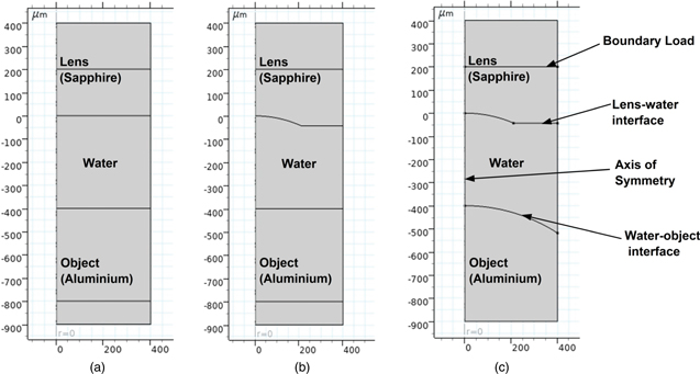
Fig. 1. COMSOL models (a) unfocused lens (flat planar lens-water interface) with flat test object (aluminum), (b) focused lens (curved lens-water interface) with flat test object. (c) Focused lens with curved test object.
Download figure:
Standard image High-resolution imageReflection of electromagnetic and elastic waves occurs at the boundary of two mediums because of the difference in the impedance between them. The acoustic impedance (Z) of a medium is defined as the product of its density (ρ) and the speed of sound (v) in that medium, i.e. Z = ρv. The greater this difference in impedance between the mediums the greater the amount of energy reflected from the boundary and the lesser is the energy that propagates in the subsequent medium. For longitudinal ultrasound, the boundary phenomenon i.e. reflection and transmission at the interface of two mediums, is similar to that of the light (electromagnetic waves).
When an ultrasonic wave from an ultrasonic transducer hits the junction of the lens-coupling medium then most of the energy (pressure amplitude) is associated with the reflected wave and only some energy is transferred as the transmitted wave. The angle of reflection is equal to that of the angle of incidence, θi = θr as well as the transmitted wave angle, θt, satisfies the condition of wavefront coherence at the boundary which yields Snell's law in acoustic, i.e. (sinθi/sinθt) = (v1/v2 ). The propagation of these waves through the boundary should not create any discontinuities in the particle's velocity or pressure. This condition leads to the following relationship for reflection (Cr ) and transmission (Ct) coefficient 14–16)


where Pi is the pressure of the incident wave, and Pr and Pt are the pressure amplitudes of reflected and transmitted waves, respectively. The reflection and transmission coefficients are dimensionless quantities and represent that the reflected wave has (Cr × 100)% of the sound pressure of the incident wave, and the transmitted wave has (Ct × 100)% pressure amplitudes. A better approach to describe these boundary phenomena can be in terms of energy rather than pressure amplitude. The intensity (i.e. the energy per unit area per unit time) of these waves is related to the pressure amplitude by the following equation 14–16)

Now, combining Eqs. (1)–(3) and considering the general case of normal incidence of acoustic waves as in the case of a plane progressive wave, for which θi = θr = θt = 0, we get the loss of energy (in dB) of the echo signal in medium 1 getting reflected from an interface boundary with medium 2 as: 17)

The loss of energy (in dB) on transmitting a signal from medium 1 into medium 2 is given by: 17)

The above formulas hold true for any flat-planar interface between two mediums as in the case of lens-water boundary of unfocused ultrasonic transducer but fails for rough-arbitrary shaped boundaries as in curved interface of focused transducers. Apart from that the ultrasonic waves attenuates as it progresses within a medium, majorly there are three causes of attenuation: absorption, diffraction, and scattering. The magnitude of attenuation through the material also plays an important role in the selection of a transducer for an application. 17–19) These effects are also not incorporated in these formulas.
In this study, we present a time-domain-based FEM model for these loss calculations. Here we have performed loss calculations for an unfocused and focused ultrasonic transducer and compared their results with the theoretical values. The material values used are given in Table I.
Table I. Material properties. 19)
| Material | Density (kg m−3) | Speed of sound (m s−1) |
|---|---|---|
| Sapphire | 3980 | 10 000 |
| Water | 998.2 | 1481.4 |
| Aluminum (Al) | 2700 | 6200 |
Theoretically, we have calculated these loss values using the impedance values calculated from the material data from Table I in Eqs. (1)–(5). Numerically the coefficients are calculated using the pressure amplitudes of the incident, reflected and transmitted wave simulated in commercially available software COMSOL Multiphysics. For simplicity, waves are considered striking at normal incidence, i.e. θi = θ r = θ t = 0. The COMSOL model here is a 2D axisymmetric model computed in the time domain. The lens dimensions and material properties are taken from the literature. 20) Three cases are chosen, i.e. an unfocused lens with a flat test object (aluminum), a focused lens with a flat test object, and a focused lens with a curved test object, as shown in Fig. 1. Acoustic solid interaction, transient physics is used, which adds the Multiphysics coupling for acoustic structure interaction. Solid mechanics physics is used for the two solid domains (lens and Al object) and pressure acoustics (transient) physics for the water domain. Acoustic-structure boundary is added at the two boundaries of interest (lens-water and water-object interface). Plane wave radiation and low-reflecting boundary conditions are used to absorb the outgoing waves in water and solid domain, respectively. The input excitation is a ricker pulse of frequency 250 MHz and pressure amplitude 1 pascal given by the following equation

where f is the excitation frequency, and t0 is 1/f. The incident, reflected, and the transmitted wave propagation can be seen in Figs. 2(a)–2(d) for the lens-water interface, and Figs. 2(e)–2(j) for the water-object interface for all the mentioned three cases.
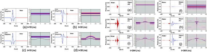
Fig. 2. (Color online) For lens-water interface (a) incident wave for the unfocused lens, (b) reflected and transmitted wave for the unfocused lens, (c) incident wave for the focused lens, (d) reflected and transmitted wave for the focused lens. Incident wave for the water-object interface (e) for the unfocused lens, (g) for the focused transducer with a flat object, (i) focused transducer with a curved object. Reflected and transmitted wave for the water-object interface (f) for the unfocused lens, (h) focused transducer with a flat object, (j) for the focused transducer with a curved object.
Download figure:
Standard image High-resolution imageThe result is shown in Table II. For a planar interface (unfocused transducer with flat test object) the theoretical and simulated result match closely. But the difference for the spherical-curved interface is huge. This huge deviation in the results is because of the scattering (diffraction) of the wave from the curved part (spherical cavity) of the lens or object, which is not accounted for in the theoretical formula. Thus, the theoretical formula fails for the calculation of reflection and transmission loss for a focused ultrasonic transducer.
Table II. Comparison of theoretical and simulated losses for the mentioned three cases.
| Lens type | dBlossecho | dBlosstransmission | ||
|---|---|---|---|---|
| Unfocused lens | Theo. | Sim. | Theo | Sim |
| Lens—water interface | −0.65 | −0.88 | −8.58 | −6.93 |
| Pi = 0.288 Pr = 0.26 Pt = 0.025 | ||||
| Water—object interface | −1.55 | −1.78 | −5.25 | −8.71 |
| Pi = 0.0215 Pr = 0.0175 Pt = 0.0265 | ||||
| Focused lens with flat object | ||||
| Lens—water interface | −0.65 | −2.72 | −8.58 | −5.07 |
| Pi = 0.288 Pr = 0.2106 Pt = 0.031 | ||||
| Water—object interface | −1.55 | 0.24 | −5.25 | 1.60 |
| Pi = 0.0574 Pr = 0.059 Pt = 0.232 | ||||
| Focused lens with curved object | ||||
| Lens—water interface | −0.65 | −2.72 | −8.58 | −5.07 |
| Pi = 0.288 Pr = 0.2106 Pt = 0.031 | ||||
| Water—object interface | −1.55 | −1.11 | −5.25 | 11.68 |
| Pi = 0.05 Pr = 0.044 Pt = 0.645 | ||||
Also, since the wave travels from a higher impedance medium to a lower impedance (in the case of lens-water interface), there is a phase reversal of π in the reflected wave which can be seen in Figs. 2(a)–2(d).
Apart from the losses, the focus on the material can also be calculated. The focus of an ultrasonic transducer is given by the formula

where RL is the radius of curvature of the lens, v1 is the speed of sound in the lens (sapphire), and v2 is the speed of sound in the coupling medium (water). The above formula is good for finding the lens's focus in a medium. However, as the ultrasonic wave travels from the coupling medium to the test specimen, as in our case the aluminum object, the focus point changes. Also, the focus point depends on the shape (curvature) of the test material. Table III presents the comparison between the focus point of the transducer for different cases. It can be seen in Figs. 3(a)–3(d), that the ultrasonic wave focuses much before in the test material, and the distance of focus increases as the radius of curvature of the test object decreases.
Table III. Focus point of the ultrasonic transducer for the radius of curvature of lens 533.25 μm.
| Focus point (F in μ m) | |
|---|---|
| Theoretical | 625.95 |
| Simulated | 625.62 |
| Flat object (Al) | 430.28 |
| Curved object R = 733.25 μm | 446.81 |
| Curved object R = 433.25 μm | 465.58 |

Fig. 3. (Color online) Focus point (point of a maximum pressure amplitude) in (a) lens with no object, (b) lens with a flat object, (c) lens with a curved object (radius of curvature of the object = 733.25 μm), (d) lens with a curved object (radius of curvature of the object = 433.25 μm).
Download figure:
Standard image High-resolution image
In this work, we have demonstrated the use of FEM based model for acoustic loss calculations at the boundary of two mediums. Here, we have used the model for the calculation of reflection and transmission loss for focused and unfocused ultrasonic transducers at the lens-water interface and water-object (test specimen) interface. In general, the model can be used for any arbitrarily shaped boundary for simulating the reflected and transmitted wave, which can be used to calculate useful parameters like these loss coefficients. Apart from this, we have also quantified the change of focal length in the test medium for flat and curved objects.
Acknowledgments
The following funding is acknowledged: Cristin Project, Norway, ID: 2061348 (Habib). The authors acknowledge the funding from Research Council of Norway, INTPART project (309802). The publication charges for this article have been funded by a grant from the publication fund of UiT The Arctic University of Norway.