
Abstract
A scanning airborne ultrasound source technique was developed to overcome the riskiness of laser ultrasound, which uses an ultrasound source that has a fixed sound wave focusing point and thus requires mechanical motion for sound source scanning. Therefore, the measurement time becomes longer. To solve this problem, we have proposed a method of simultaneously exciting many measurement points in the target using focused ultrasound sources of different frequencies. In this paper, we investigated the visualization of defects in a thin metal plate by the scanning elastic wave source technique using an airborne ultrasound source driven at two frequencies. When the testing was performed using two frequencies, either frequency visualized the defects.
Export citation and abstract BibTeX RIS
1. Introduction
Non-destructive testing methods for various objects in various situations have been developed. 1–7) In the ultrasound method, the test target is irradiated with ultrasound waves using a contact transducer and a coupling material, and defects in the test target are detected by observing or imaging the reflected echo. 8) This method enables highly accurate testing, although the measurement area is limited to the dimensions of the transducer. Therefore, the method is too lengthy for large metal structures, such as pipes and tanks in power plants and chemical plants. A testing method using guided waves that can shorten the measurement time has been developed.
Guided waves are a type of ultrasound that propagate through solid materials, and when the material is thin with respect to the wavelength of the propagating sound waves, Lamb waves are generated. 9) Lamb waves are propagated over long distances by energy traps, and are used for testing large areas. 10)
Non-contact methods for exciting guided waves that do not require a coupling material and are not easily affected by the surface roughness of the object have been proposed. The methods use laser ultrasound, 11,12) an electromagnetic acoustic transducer, 13,14) and an air-coupled ultrasound. 15–20) The laser ultrasound method is practical from the perspective of long-distance irradiation, and a scanning laser source technique for visualizing defects in thin metal has been developed. 21–24) In this technique, the target is irradiated with a low-frequency pulsed laser from a distance, and the laser irradiation point (excitation source) is scanned at high speed in the measurement area by galvano mirror scanning. The elastic waves generated from each excitation point on the target surface are measured by an ultrasound probe or a laser Doppler vibrometer fixed on the target surface. This measurement method relies on reciprocity, and thus it is not necessary to scan the position where the Lamb wave is received, allowing stable high-speed measurement. However, this method can damage the target by laser ablation and the configuration and control of the measurement device are complicated.
To solve these problems with laser ultrasound, Osumi et al. developed a scanning elastic wave source technique using airborne ultrasound. 25) Airborne ultrasound uses longitudinal waves generated by compression and expansion of air; therefore, non-contact excitation of guided waves is possible without damaging the target.
Wideband imaging with airborne ultrasound that exploits the strong non-linear characteristics of high-intensity ultrasound has been developed. The point-focused airborne ultrasound source used in this measurement method has a fixed sound wave focusing point. 17,18,25) Accordingly, the sound source scanning requires mechanical motion, which causes long measurement times.
To overcome this limitation, a scanning elastic wave source technique using an airborne ultrasound phased array (AUPA) was developed. 26–28) An AUPA consists of many ultrasound emitters arranged in a square. By appropriately controlling the input signal to the ultrasound emitters, the sound waves can be focused at any point directly above the AUPA. AUPAs have mainly been used in ultrasonic levitation 29) and tactile presentation. 30,31) However, Shimizu et al. applied an AUPA to non-destructive testing and detected thinning defects that occur in thin metal plates and have dimensions similar to the wavelength of Lamb waves. In addition, we reduced the testing time, which used to take 60 min or more in the conventional method, to several minutes. 27)
The time required for testing in the scanning wave source technique is determined by the scanning speed of the wave source. The measurement time can be reduced by shortening the interval from the excitation of the guided wave at the point in the measurement area to the excitation of the guided wave at the next point. However, in a test target of finite dimensions, reflected waves are generated at the edge of the target, and multiple guided waves are scattered in the target. If the guided wave is generated at the next points before the scattered guided wave is sufficiently attenuated, the guided waves interfere with each other creating an artifact in the visualization and accurate measurement cannot be performed. 12) Thus, there is a trade-off between test speed and test accuracy. To shorten the testing time while maintaining the testing accuracy, multiple points in the target could be excited simultaneously. This method has been used in medical ultrasound, 32–36) but it has never been applied in guided wave measurement using airborne ultrasound. This is because when multiple excitation points are excited by sound waves of the same frequency, the guided waves generated at each excitation point cannot be distinguished and accurate testing results cannot be obtained.
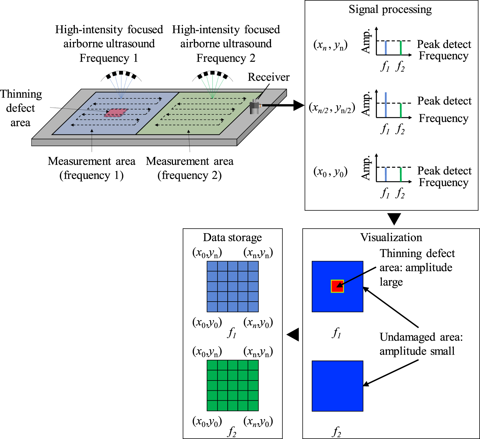
We have proposed a method of simultaneously exciting many points in the target using focused ultrasound sources of different frequencies. The waveform shape of guided waves changes depending on its dispersity, but its frequency component does not. Therefore, by simultaneously exciting the target at different frequencies and distinguishing the received guided wave waveform in the frequency domain by using Fourier transformation, the guided wave information corresponding to the excitation point can be obtained. Figure 1(b) shows the proposal measurement system using AUPA. When each measurement point is vibrated sequentially, as in the scanning laser source technique, it is necessary to wait for the attenuation of sound wave scattering at each measurement point, which increases the measurement time [Fig. 1(a)]. Our method addresses this problem by dividing the AUPA into multiple sections and scanning the wave source to realize high-speed imaging of defects in thin metal plates by using the AUPA driven at multiple frequencies.

Fig. 1. (Color online) Schematic of the proposed method using an AUPA. (a) Scanned with a single frequency. (b) Scanned with multiple frequencies.
Download figure:
Standard image High-resolution imageAt the 42nd Symposium on Ultrasonic Electronics, as a preliminary study of our method, we visualized defects with two frequencies of guided waves. 35) In this paper, we investigated the practical visualization of defects about the size of the wavelength of the guided waves in a thin metal plate by the scanning elastic wave source technique using airborne ultrasound waves driven at two frequencies.
2. Scanning elastic wave source technique using guided waves of multiple frequencies
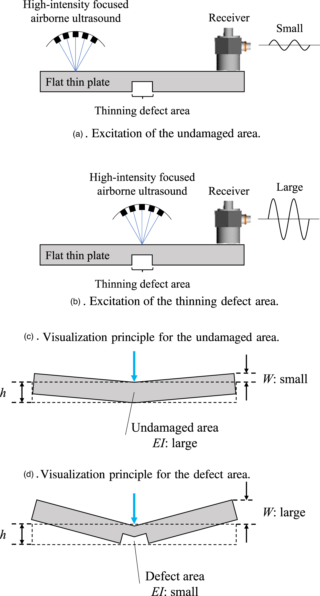
Generally, when the sound waves are transferred from air into a solid, the difference in acoustic impedance between the air and the solid is large, and the incident efficiency of the sound wave on the solid is small (1% or less). However, non-contact excitation of a thin metal plate with guided waves is possible using high-intensity airborne ultrasound. Sound waves that enter the solid cause mode conversion at the boundary between the air and the solid. When the solid is a thin plate, Lamb waves are generated, which in a thin plate of finite length, are mainly A0 mode waves (Fig. 2). The speed of the A0 mode of Lamb waves is expressed by the following equations. 9)


Here, C is the Lamb wave velocity, ω is the frequency, k is the wavenumber, CL is the longitudinal wave propagation velocity, CT is the transverse wave propagation velocity, and d is the thickness of the flat plate. For example, in the case of duralumin, assuming that CL is 6300 m s−1, CT is 3100 m s−1, and d is 3 mm, the speed of the Lamb wave is calculated from Eqs. (1) to (4). The speed of sound of a 40 kHz Lamb wave is about 1080 m s−1, and that of a 60 kHz Lamb wave is about 1330 m s−1. The speed of sound varies from frequency to frequency due to the dispersibility of Lamb waves. Therefore, the wavelength of the Lamb wave propagating in the target is about 27 mm at 40 kHz and about 22 mm at 60 kHz.

Fig. 2. (Color online) Generation of guided waves by high-intensity focused airborne ultrasound. (a) Excitation of the undamaged area. (b) Excitation of the thinning defect area. (c)Visualization principle for the undamaged area. and (d) Visualization principle for the defect area.
Download figure:
Standard image High-resolution imageNow, consider a thin metal plate with defects that is irradiated with sound waves. When the undamaged area is excited [Fig. 2(a)], the bending rigidity of the plate is large, so the vibration displacement of the generated Lamb wave is small, and the signal received by the acoustic emission (AE) sensor is small. However, when the area around the thinning defect area is excited [Fig. 2(b)], the bending rigidity is smaller than that in the undamaged area, so large vibration displacement occurs and the signal becomes large. This phenomenon allows an image of the shape of the thinning defect area to be obtained from the peak distribution of the signal received by the AE sensor when each position in the measurement area in the thin plate is excited. Based on these principles, simultaneous measurement is performed on an object using multiple-frequency ultrasound.
Figure 3 shows the generation of guided waves in the thin metal plate by airborne ultrasound irradiation at two different frequencies. Figure 3(a) shows the excitation of the undamaged area of the target by a sound wave of frequency f1. The frequency component of the received wave in the AE sensor is f1, and its amplitude is small. Figure 3(b) shows the excitation of the thinning defect area of the target by a sound wave of frequency f2. The frequency component of the received wave in the AE sensor is f2, and its amplitude is larger than that in the undamaged area. If an object is excited simultaneously with sound waves of frequencies f1 and f2 [Fig. 3(c)], the excitations shown in Figs. 3(a) and 3(b) are superimposed.

Fig. 3. (Color online) Generation of guided waves by multiple-frequency high-intensity focused airborne ultrasound. Excitation of the thinning defect area with (a) Excitation of the thinning defect area, (b) Excitation of the thinning defect area, and (c) Excitation of the thinning defect area.
Download figure:
Standard image High-resolution imageFigure 4 shows the point-focused sound waves of two frequencies simultaneously scanned and irradiated in each area of one object. The guided wave generated on the target is received by the AE sensor fixed on the surface of the target and the received wave signal is Fourier transformed to detect the peak value of the frequency corresponding to the drive frequency of the sound source. These results obtained by scanning the sound source are stored in the array corresponding to the sound wave irradiation coordinates.

Fig. 4. (Color online) Overview of the visualization by the proposed method.
Download figure:
Standard image High-resolution imageThe visualization of defects by this amplitude ratio can be understood by the static bending of the beam (Fig. 1). The displacement, W, of the beam caused by the irradiation of sound waves is expressed by Eq. (5). Here, M is the bending moment generated by sonic irradiation, E is the Young's modulus, and I is the moment of inertia of the area. EI is also called the flexural rigidity. 36) I is expressed by Eq. (6). Because thickness h of the beam changes between the undamaged area and the thinning defect area, W changes in proportion to the cube of h according to Eq. (5). 36) W is inversely proportional to the cube of h, and thus the defect can be visualized from the ratio of W in the undamaged area to that in the defect area. The guided wave generated at each measurement point propagates while maintaining energy. 21) That is, the amplitude of the guide wave received by the AE sensor is determined by the plate thickness at the measurement point.


Based on these results, we acquired visualization images with and without defects in the measurement area.
3. Experimental verification
3.1. Outline and characteristics of the ultrasound source
3.1.1. Creating sound sources
Two point-focused airborne ultrasound sources were created to generate guided waves on the thin metal plate. The sound sources consisted of 100 ultrasound emitters (UT1007-Z325, SPL (Hong Kong) Limited; resonance frequency 40 kHz) arranged on part of a spherical surface with a diameter of 150 mm (Fig. 5). In addition, sound waves were radiated through an acoustic guide consisting of an acoustic window (2 mm thick, acrylic) and a pipe (acrylic, 45 mm long, 6 mm inner diameter) to prevent the effects of side lobes that occur with sound wave focusing.

Fig. 5. (Color online) Schematic view of the sound source. (a) Perspective view. (b) Top view.
Download figure:
Standard image High-resolution imageFigure 6 shows the impedance characteristics of the ultrasound emitter measured by an LCR meter (ZM2376, NF Corporation). Impedance measurements were taken over a frequency range of 20–100 kHz in 50 Hz steps. The resonance state was observed around 40 kHz and the second resonance was present, even around 60 kHz. That's the reason why sound source SS1 was driven at a frequency of 40 kHz and SS2 was driven at a frequency of 60 kHz.

Fig. 6. Frequency-impedance characteristics of the ultrasound emitter.
Download figure:
Standard image High-resolution image3.1.2. Sound source radiation characteristics
The sound wave radiation characteristics of the sound sources were measured using the experimental equipment shown in Fig. 7(a). The equipment was a 1/8 in. condenser microphone (40DP, GRAS), a preamplifier (Type 12AA, GRAS), a data logger (PXIe-5172, NI; sampling frequency, 2 MHz; number of samples, 10 000), a precision stage (SGSP46, Sigma Koki), a stage controller (SHOT-204MS, Sigma Koki), a function generator (WF1974, NF), an amplifier (HAS 4051, NF), and a personal computer. A burst wave with a frequency of 40 kHz and 10 cycles was input to SS1, and a burst wave with a frequency of 60 kHz and 10 cycles was input to SS2, and both sound sources were driven. The sound pressure with respect to the applied voltage was measured at the position indicated by the red dot in Fig. 7(b). In addition, the sound pressure distribution of the radiated sound waves near the open end of the acoustic guide in the range shown in blue was measured by scanning the microphone. The instantaneous sound pressure distribution at the time when the sound pressure reached its maximum was extracted.

Fig. 7. (Color online) Schematic of the measurement device for the sound source characteristics. (a) Measuring device configuration. (b) Measurement area.
Download figure:
Standard image High-resolution imageFigure 8 shows the sound pressure characteristics at the open end of the acoustic guide with respect to the applied voltages of sound sources SS1 and SS2. The generated sound pressure was proportional to the applied voltage of the sound source. A sound pressure of about 1000 Pa was generated in SS1 at an applied voltage of 6.7 VP-P and in SS2 at an applied voltage of 9.7 VP-P.

Fig. 8. (Color online) Sound pressure characteristics with respect to applied voltage.
Download figure:
Standard image High-resolution imageFigures 9(a) and 9(b) show the sound pressure distribution of radiated sound waves near the open ends of the acoustic guides of SS1 and SS2, respectively. The result is the normalized sound pressure distribution at the timing of the maximum sound pressure of 1000 Pa. The distributions showed that high-intensity sounds were radiated in almost the same range as the inner diameter of the pipe in all the results.

Fig. 9. (Color online) Normalized instantaneous sound pressure distribution of the sound sources. (a) SS1 (40 kHz). (b) SS2 (60 kHz).
Download figure:
Standard image High-resolution imageFigure 10(a) shows the time waveform of the sound pressure at the open end of the acoustic guide of SS1, and Fig. 10(b) shows the frequency spectrum of (a), in which the maximum peak occurred at the drive frequency of 40 kHz and there were small peaks at 60 and 80 kHz. The peak at 60 kHz was the sound wave of the second resonance of the sound source, and was generated by inputting a burst wave with a wide band. The 80 kHz peak was the second harmonic and was generated by the non-linearity of the sound waves. The peaks generated at 60 and 80 kHz were less than 1/5 of the peak amplitude of 40 kHz.

Fig. 10. Characteristics of SS1. (a) Normalized waveform. (b) Normalized frequency spectrum.
Download figure:
Standard image High-resolution imageFigure 11(a) shows the time waveform of the sound pressure at the open end of the acoustic guide of SS2, and Fig. 11(b) shows the frequency spectrum of (a), in which the maximum peak occurred at the drive frequency of 60 kHz and there was a small peak at 40 kHz. This was the first resonance sound wave of the sound source, which was generated by inputting a burst wave with a wide band to the sound source.
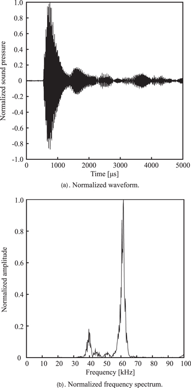
Fig. 11. Characteristics of SS2. (a) Normalized waveform. (b) Normalized frequency spectrum.
Download figure:
Standard image High-resolution imageThe results showed that the frequency component contained in the sound waves of both sound sources was dominated by the component of the drive frequency of the sound source.
3.2. Attempt to image thinning defects
3.2.1. Experimental equipment and method
Using the experimental equipment shown in Fig. 12, we visualized a thinning defect in a thin metal plate. The device consisted of the two point-focused high-intensity airborne ultrasound sources (mentioned in Chapter 3.1., drive frequencies of 40 and 60 kHz), a precision stage (SGSP46, Sigma Koki), a stage controller (SHOT-204MS, Sigma Koki), an AE sensor (PICO, Physical Acoustics) for receiving guided waves, a preamplifier (2/4/6 C, MISTRAS), a data logger (PXIe-5172, NI; sampling frequency, 2 MHz; number of samples, 4000), a function generator (USB-6363, NI), an amplifier (HAS 4051, NF), and a personal computer. The measurements were performed by scanning the target sample mounted on the precision stage.

Fig. 12. (Color online) Schematic of measurement device for visualization. 35) (a) Measuring device configuration. (b) Measurement details.
Download figure:
Standard image High-resolution imageFigure 13 shows schematics of the samples used in this experiment. The samples were made of duralumin and measured 1000 × 300 × 3 mm, sample 1 had a thinning defect of 80 × 50 × 0.5 mm at the position shown in Fig. 13(a), and sample 2 had a thinning defect of 20 × 20 × 0.5 mm at the position shown in Fig. 13(b). The measurement areas were two areas of 300 × 100 mm (excitation areas 1 and 2). These two areas were individually scanned and irradiated with sound waves at frequencies of 40 and 60 kHz, respectively, and the guided waves were excited. Guided waves excited in the sample were received by the fixed AE sensor and the FFT was performed by the computer on the entire measured waveform. Reference 12 shows that defects can be visualized even when the FFT is performed on the measured waveform including the reflected wave generated at the edge of the sample.

Fig. 13. (Color online) Samples and measurement areas. (a) Sample 1. 35) (b) Sample 2.
Download figure:
Standard image High-resolution imagePeak values around 40 and 60 kHz were extracted from the results and were acquired as a two-dimensional array with the coordinate information for the guided wave sound wave irradiation. The experiment was performed on the entire measurement area (excitation areas 1 and 2), and a visualization image of the measurement was obtained from a peak value distribution.
4. Results and discussion
Figure 14 shows the visualization results for sample 1. Figure 14(a) shows the results of the excitation of excitation area 1 at 40 kHz and excitation area 2 at 60 kHz. In the measurement area including the defect area excited at 40 kHz, the amplitude was increased in the defect area and the defect area was visualized. However, in the undamaged measurement area excited at 60 kHz, the amplitude did not increase and it was visualized as undamaged. Figure 14(b) shows the results of exciting excitation area 1 at 60 kHz and excitation area 2 at 40 kHz. In the measurement area including the defect area excited at 60 kHz, the amplitude was increased in the defect area and the defect area was visualized. In the undamaged measurement area excited at 40 kHz, the amplitude did not increase and it was visualized as undamaged. The results showed that the frequencies could be distinguished and the defects were visualized even when the frequencies were exchanged, indicating that high-speed defect visualization using AUPA could be achieved.

Fig. 14. (Color online) Visualization results for sample 1. 35) (a) Excitation area 1 at 40 kHz and excitation area 2 at 60 kHz. (b) Excitation area 1 at 60 kHz and excitation area 2 at 40 kHz.
Download figure:
Standard image High-resolution imageFigure 15 shows the visualization results for sample 2. Figure 15(a) shows the results of exciting excitation area 1 at 40 kHz and excitation area 2 at 60 kHz, and Fig. 15(b) shows those of excitation area 1 at 60 kHz and excitation area 2 at 60 kHz. In both results, the amplitude was increased in the defect area and the defect area was visualized.

Fig. 15. (Color online) Visualization results for sample 2. (a) Excitation area 1 at 40 kHz and excitation area 2 at 60 kHz. (b) Excitation area 1 at 60 kHz and excitation area 2 at 40 kHz.
Download figure:
Standard image High-resolution image
The results demonstrate that the proposed method can measure twice the range of the conventional method in one measurement because the measurement time is half that of the conventional method. Our method is effective because it can detect thinning defects with a dimension of about the wavelength of the target 40 kHz Lamb wave.
5. Conclusions
To achieve high-speed non-destructive inspection of thin metal plates using an AUPA, we visualized defects in thin metal plates by a scanning elastic wave source technique using multiple airborne ultrasound sources driven at different frequencies. Defects in the metal sheet were visualized using many frequencies and the measurement range for one measurement was twice that of the conventional method, demonstrating that our method is effective.
Acknowledgments
This work was partly supported by JSPS KAKENHI Grant No. 19K04931.