
Abstract
In a previous study, an annular-array transducer was employed to characterize homogeneous scattering phantoms and excised rat livers using backscatter envelope statistics and frequency domain analysis. A sound field correction method was also applied to take into account the average attenuation of the entire scattering medium. Here, we further generalized the evaluation of backscatter coefficient (BSC) using the annular array in order to study skin tissues with a complicated structure. In layered phantoms composed of two types of media with different scattering characteristics, the BSC was evaluated by the usual attenuation correction method, which revealed an expected large difference from the predicted BSC. In order to improve the BSC estimate, a correction method that applied the attenuation of each layer as a reference combined with a method that corrects based on the attenuation of the analysis position were applied. It was found that the method using the average attenuation of each layer is the most effective. This correction method is well adapted to the extended depth of field provided by an annular array.
Export citation and abstract BibTeX RIS
1. Introduction
Quantitative ultrasound (QUS) assessment based on ultrasound backscattering properties and propagation characteristics is a useful technique for non-invasive evaluation of disease of various biological tissues such as liver, 1–4) breast, 5–8) lymph node, 9,10) and skin. 11,12) Clinically focused QUS methods can be divided into elastography, 13–17) amplitude envelope statistics, 18–21) and frequency domain analysis. 22–24) In frequency domain analysis, the physical parameters of the scattering source are estimated by comparing the theoretical model of the backscatter coefficient (BSC) to the frequency characteristics of the measured backscatter signal. 25,26) Theoretically, the BSC includes the scatterer structure information, such as the diameter, shape, concentration of scatterers, and acoustic impedance between the scatterers and surrounding media. The BSC is calculated after compensating for the system properties and acoustic attenuation in order to provide a system independent measurement.
In general, clinical scanners with linear array probes or custom scanners with single-element focused transducers are used in QUS research. Linear arrays entail complicated transmission and reception conditions and single-element transducers have a limited depth range for reliable QUS measurements. 27,28) Annular-array transducers, with their extended depth of field (DOF) and radial symmetric beam profile provide a way to overcome these limitations. Annular arrays have been applied to ophthalmological, 29,30) small-animal, 31,32) and photoacoustic, 33,34) imaging. However, there limited studies that apply QUS methods to backscatter data acquired with annular arrays.
In our previous studies, we performed amplitude envelope statistics and frequency domain analysis of homogeneous scattering phantoms and excised rat livers using a 20 MHz HFU annular-array transducer. The extended DOF achieved with the annular arrays was found to improve the estimation accuracy of QUS parameters compared to the fixed-focus case. 35,36) Here, a HFU annular-array transducer was applied to QUS analysis for skin tissues with layered structure. 37) In the BSC analysis, the reference phantom method (RPM) was applied to remove the effect of the ultrasound system. 38) The BSC was evaluated from the acquired RF signals observed from homogeneous two-layer phantoms that simulate the difference in acoustic impedance between the dermis and hypodermis. The effect of the thickness of the upper phantom on the evaluation accuracy of BSC was investigated. In addition, because attenuation correction has a strong effect on the BSC, two types of correction methods were applied, and the results were compared.
2. Materials and methods
2.1. Annular array and synthetic focusing
The annular-array transducer used in this study had 5 equal area elements with a center frequency of 20 MHz. The fabrication methods of the HFU annular array transducer were described in Ketterling et al. 39) The annular array had a 10 mm total aperture, a 31 mm geometric focus, and a 100 μm spacing between each the annuli.
Synthetic focusing (SF) with a delay and sum process was employed to improve DOF and resolution.
40) In the SF method, the acquired echo data set was post-processed and the 25 pairs (transmit (Tx) * receive (Rx) channels) of the RF signals are time shifted and summed. At an arbitrary focal point  the delay
  of the
  th annuli is computed follows as:
41)
th annuli is computed follows as:
41)

where  is the average radius of the
  th element,
  is the geometric focal length and
  is the speed of sound. Note that the round-trip delay time is written in
  where
where  is transmit
  th channel and
  is receive
  th channel.
For a final image with  samples, the SF algorithm is described by

where  is the RF signal for transmitting the
  th and receiving the
  th channel. If the RF signals are summed without a delay shift (
 ), the beam profile is the same as a single-element focused transducer with the same total aperture and geometric focus as the annular array transducer. The acoustic specification of the annular array transducer was the same as our previous study.
35) The lateral beam profile was measured by scanning the annular array across the wire.
42) Figure 1 shows the maximum amplitude and lateral resolution at each wire position in the depth direction with the two focusing methods (synthetic and fixed focusing). The DOF was determined within the range of −6 dB from the maximum intensity of the echo envelope. The DOF was expanded 5–17 mm [Fig. 1(a)], and the improvement of the lateral resolution was also evident [Fig. 1(b)] after applying the SF technique.
), the beam profile is the same as a single-element focused transducer with the same total aperture and geometric focus as the annular array transducer. The acoustic specification of the annular array transducer was the same as our previous study.
35) The lateral beam profile was measured by scanning the annular array across the wire.
42) Figure 1 shows the maximum amplitude and lateral resolution at each wire position in the depth direction with the two focusing methods (synthetic and fixed focusing). The DOF was determined within the range of −6 dB from the maximum intensity of the echo envelope. The DOF was expanded 5–17 mm [Fig. 1(a)], and the improvement of the lateral resolution was also evident [Fig. 1(b)] after applying the SF technique.

Fig. 1. (Color online) The beam profiles of the annular array; (a) the maximum amplitude of the echo signal from the wire and (b) the lateral resolution.
Download figure:
Standard image High-resolution image2.2. Skin mimicking two-layer phantoms
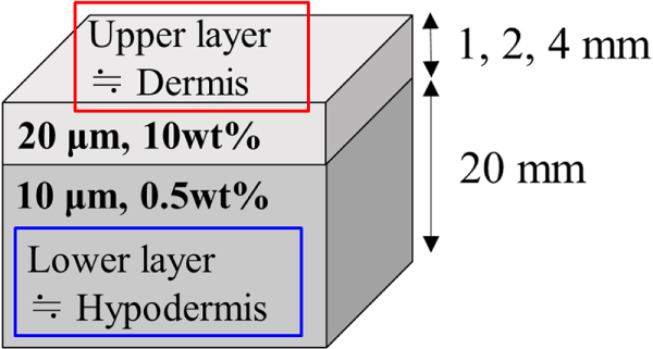
The homogeneous upper layer phantoms were made in a rectangular case (width × length × height = 8 cm × 0.1, 0.2, 0.4 cm × 4 cm) 28) as a mixture of 2% wt distilled water, agar powder (A1296; Sigma-Aldrich, MO, USA), and 10% wt acrylic scatterers with a mean diameter of 20 μm (MX-2000; Soken, Aichi, Japan). In the lower phantoms, 0.5% wt nylon scatterers with a mean diameter of 10 μm (ORGASOL 2002 EXD NAT 1; Arkema, Colombes, France) was used. The theoretical acoustic impedances of the upper and lower layer are 1.6659 and 1.4937 MRayl, respectively. The acoustic conditions of the upper layer and the lower layer were determined to match the dermis and the hypodermis, respectively. A skin tissue was expressed by stacking two layers (Fig. 2). The interface between dermis and hypodermis is clear in the clinical high-frequency imaging of skin. However, the interface between the upper and lower layer was unclear in this study. This was because the boundary between the two phantoms was uneven due to some slight mixing caused by the heat applied when joining the two phantoms sections. This situation simulates skin disorders such as lymphedema where border echoes become unclear. 43) However, compared to the degeneration and mixing of living tissues in skin diseases, the mixing of boundary sites in the two-layer phantoms are small. The two-layer phantoms with the upper layer thickness of 1, 2, and 4 mm were named phantom I, II, and III, respectively. The single-layer phantom used as the reference phantom (Phantom IV) had no upper layer and was composed only of substances with the same composition as the lower layers of phantoms I to III.

Fig. 2. (Color online) Schematic diagram of the homogeneous two-layer phantoms. The upper and the lower layer expresses dermis and hypodermis in skin tissue, respectively.
Download figure:
Standard image High-resolution imageThe speed of sound and attenuation coefficient of each layer were calculated from the echo signal measured by a planar transducer (V313; Olympus, Tokyo, Japan,) using the standard substitution method. 44) The attenuation coefficient (AC) was estimated at 8–17 MHz.
2.3. Data acquisition using laboratory-made scanner
Three-dimensional RF data sets observed with all 25 transmit-receive ring pairs were acquired by scanning the annular array transducer using a laboratory-made ultrasonic scanner. 35) The transducer was mechanically scanned using a three-axis linear motor stage (MTN100CC; Newport, CA, USA). The scanning pitch was 30 μm in each direction. For the acquisition of echo signals from each phantom, one element was excited with a negative impulse from a pulser/receiver (Model 5800; Olympus, Tokyo, Japan) and the echo was received by one of the five elements filtered with a 1–35 MHz band-pass filter. The energy level of the pulser was 12.5 μJ. Each echo signal was digitized at a 250 MHz sampling rate with 12 bits/sample by a digital storage oscilloscope (HDO6104; Teledyne LeCroy, NY, USA). All data acquisition was controlled using LabVIEW (National Instruments, TX, USA). Degassed water at 22 °C–24 °C was used to couple the transducer the phantom.
2.4. Backscatter coefficient analysis
The frequency characteristics of the backscatter signal evaluated from echo signal observed by the annular-array transducer include the characteristics of the measurement system (i.e. acoustic field and electrical circuit) and the scatterers in the scattering medium. In order to cancel the characteristics of the measurement systems and evaluate the BSCs in the upper and lower layers, the RPM was employed.
38) The measured BSC value  was estimated from a region of interest (ROI) defined as

where  is the average of the power spectrum of several adjacent lines in the ROI,
  is the power spectrum from a reference phantom, and
  is the frequency.
  is the theoretical BSC estimated by a solid sphere model (Faran's theory).
45) The attenuation function of a measurement object
is the theoretical BSC estimated by a solid sphere model (Faran's theory).
45) The attenuation function of a measurement object  shown in Eq. (6) is a function which compensates for acoustic attenuation from the transducer surface to the upper portion of the ROI and the attenuation in withing the ROI, and is defined as
where  is the AC,
  is propagation distance.
  is the length of the ROI that is windowed using a Hanning window. The attenuation function of the reference medium
  also compensate the RF signals from reference phantoms.
The mean deviation [dB] from the theoretical BSC  was calculated as the benchmark of the BSC variations among the upper layer thickness. The mean deviation was defined as
46)
was calculated as the benchmark of the BSC variations among the upper layer thickness. The mean deviation was defined as
46)

where BW is the set of frequencies in the analyzed bandwidth.
2.5. Attenuation coefficient estimation
The local ACs in each ROI in the upper and lower layers were evaluated using the spectral log-difference technique based on the RPM.
38) The backscattered power spectra,  is defined as the product term of beam profile
 and attenuation function with the exponential term in frequency
  domain.

where  is AC at the local depth
  The logarithm of Eq. (9) is defined as

The method begins by considering the backscattered power spectra from local regions in the two mediums: one at the proximal edge of the window,  and the other at the distal edge of the window,
  The normalized power spectra divide those of the local regions in an analyzed medium by corresponding spectra from a reference phantom as

where the method assumes a constant  that is
  regardless of the different depth
  and
and  The unknown tissue AC
  in the frequency domain is solved by unknown
  in the reference phantom
The AC [dB/cm/MHz] can be obtained assuming the linear slope of the attenuation versus frequency.
The power spectra from each window were averaged with those from adjacent scan lines at each depth to estimate the power spectra  and
and  in the target and reference phantom data. The constant
  of 0.13 dB cm−1 MHz−1 was taken from the mean of the analyzed total attenuation in the standard substitution method
44) (same as the Sect. 2.2). The attenuation coefficient was estimated using the least-squares method in the range 8–17 MHz. The length
of 0.13 dB cm−1 MHz−1 was taken from the mean of the analyzed total attenuation in the standard substitution method
44) (same as the Sect. 2.2). The attenuation coefficient was estimated using the least-squares method in the range 8–17 MHz. The length  was constant to 1, 2, and 4 mm.
In this study, total AC over the entire phantom and two types of local AC (Fig. 3) were calculated, and the BSC evaluation results from each were compared. The local AC was layer averaged AC and was calculated from the echo signal as the attenuation at all depths of the upper and lower layers. The other local AC was partial, very short-range attenuation within a small three-dimensional ROI (0.54 × 0.54 mm2 in lateral direction and 0.75 mm in depth direction) for assessing the BSC. The composition of the two-layer phantoms, total AC, and layer averaged AC of each phantom are shown in Table I.
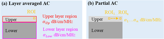
Fig. 3. (Color online) Schematic diagram calculating methods of local ACs; (a) layer averaged AC and (b) partial AC.
Download figure:
Standard image High-resolution imageTable I. Composition and ACs of the two-layer phantoms.
| Name | Thickness of upper layer [mm] | Thickness of lower layer [mm] | Total AC [dB/cm/MHz] | Layer averaged AC of upper layer [dB/cm/MHz] | Layer averaged AC of lower layer [dB/cm/MHz] |
|---|---|---|---|---|---|
| Phantom I | 1 | 20 | 3.06 | 0.01 | 0.78 |
| Phantom II | 2 | 20 | 2.95 | 0.18 | 0.56 |
| Phantom III | 4 | 20 | 2.84 | 0.39 | 0.23 |
| Phantom IV | 0 | 20 | 0.13 | — | — |
Scatterer diameter: 20 μm upper layer, 10 μm lower layer.
3. Results and discussion
3.1. BSC evaluation using total AC for attenuation correction
Figure 4 shows ultrasound images from each phantom. Figure 4(a) demonstrates the amplitude on lower layer was smaller than the upper layer regardless of the focus depth. In addition, it can be confirmed that the deep area of Phantom II and III is clearly affected by the attenuation by the upper layer compared to Phantom I. On the other hand, in Fig. 4(b) which is the observation result of the single layer homogeneous Phantom IV shows that the annular array can maintain good sound pressure over a wide range. From this comparison result, it can be understood that strong scattering occurs in the upper layer in each two-layer phantom. In the lower layer of each two-layer phantom, the amplitude of the echo signal was much lower than that of the upper layer. However, it was about 3 dB larger than the noise. Therefore, the signal required for BSC analysis could be acquired.
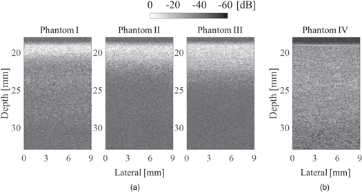
Fig. 4. B-mode images of phantoms; (a) two-layer phantoms I–III and (b) single-layer phantoms IV.
Download figure:
Standard image High-resolution imageFigure 5 represents the result of BSC evaluation using Phantom IV as the reference medium. Figures 5(a) and 4(b) show the BSC curves in the upper and lower layer, respectively. The blue, red, and green lines represent calculated BSCs of two-layer phantoms with the upper layer thickness 1, 2, and 4 mm, respectively. The black dashed line indicates the theoretical line of the upper layer in Fig. 5(a) and lower layer in Fig. 5(b). The theoretical BSC was calculated using the known parameters of the Faran model: speed of sound through the particles = 2730 m s−1, particle density = 1.19 g cm−3, Poisson coefficient = 0.35, particle diameter = 20 μm, speed of sound in the surrounding medium = 1500 m s−1, medium density = 1.0 g cm−3, and the volume fractions of 10% wt in the upper layer. The speed of sound through the particles was 2200 m s−1, particle density = 1.01 g cm−3, Poisson coefficient = 0.42, particle diameter = 10 μm, the speed of sound in the surrounding medium = 1500 m s−1, medium density = 1.0 g cm−3, and the volume fractions of 0.5% wt in the lower layer. 45)
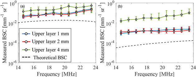
Fig. 5. (Color online) Average value of the measured BSC using total AC for attenuation correction in both layers; (a) the upper layer and (b) the lower layer.
Download figure:
Standard image High-resolution imageThe BSCs in both layers were affected by the thickness of the upper layer. In the upper layer, the BSC was about 1-2 dB larger than the theoretical value in any thickness of the upper layer. This was because the scattering intensity of the target phantoms were higher than that of the reference medium. The reason why the result was significantly different from the other two when the thickness was 4 mm was because the strong scattering signal interference inside the upper layer gave a stronger echo than the other cases. On the other hand, in the lower layer, BSCs were evaluated to be about 2–4 dB larger than the theoretical value. This was because the power of the ultrasonic wave that reached the lower layer became smaller when the upper layer was thick, and the difference of attenuation of the reference medium between the theoretical value and the observation value became larger. Therefore, it is necessary to apply high power to the lower layer using a system that can irradiate high sound pressure when the upper layer is thick or apply a correction method when the attenuation is extremely large.
In general, absorption attenuation dominates the attenuation of ultrasonic waves in homogeneous media such as biological soft tissues. However, our phantoms, based on water and agar, did not use any chemicals that regulate attenuation. Therefore, the attenuation coefficient of the phantoms was dominated by the scattering attenuation caused by the strongly scattering acrylic spheres. Strong reflections at the boundary between the upper and lower layers could also have a strong effect on attenuation. However, the boundary reflection was not as strong as in healthy skin (Sect. 2.2) which indicates the effect of the boundary reflection was not significant in our phantoms.
3.2. BSC evaluation using local AC for attenuation correction
Figure 6 represents the results of BSC evaluation using Phantom IV as the reference medium and using the layer averaged ACs of upper and lower layers. The presentation methods for Figs. 6(a) and 6(b) are the same as for Figs. 5(a) and 5(b), respectively. In the upper layer, the BSCs showed almost the same value at all thicknesses. This was due to the use of standardized attenuation in each phantom, which was a natural result. Even in the lower layer, there was no significant difference due to the thickness of the upper layer confirmed in Fig. 5(b). On the other hand, the frequency dependence of BSC was clearly shown. This result may be reasonable considering that the power of the ultrasonic waves reaching the lower layer was smaller than that of the reference phantom and that the scattering in the upper layer was large. However, it remains a question whether the lack of dependence on the different thicknesses of the upper layers was the correct result.

Fig. 6. (Color online) Average value of the measured BSC using layer-averaged AC for attenuation correction in each layer; (a) the upper layer and (b) the lower layer.
Download figure:
Standard image High-resolution imageIn order to address that question, Fig. 7 shows the result of evaluating BSC using the partial AC calculated for each ROI for attenuation correction. Similar to Figs. 5 and 6, Fig. 7(a) is the evaluation result of the upper layer, and Fig. 7(b) is the evaluation result of the lower layer. The tendency of Fig. 7(a) as the mean value and the standard deviation (SD) is almost the same as that of Fig. 6(a). This means that in the upper layers with different thicknesses, the scattering characteristics within the layers were nearly homogeneous in each phantom, respectively. On the other hand, Fig. 7(b) shows that the BSC of the lower layer differs greatly depending on the thickness of the upper layer. In order to interpret this result, it is necessary to understand the detailed information of partial AC.
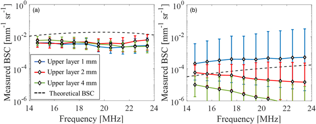
Fig. 7. (Color online) Average value of the measured BSC using partial AC for attenuation correction in each layer; (a) the upper layer and (b) the lower layer.
Download figure:
Standard image High-resolution imageFigure 8 shows the parametric images of the estimated partial AC in each ROI. The extended DOF results in a point spread function varies only slowly with depth. However, the sound pressure is not a constant as the depth varies. As predicted earlier, the AC in the upper layer was homogeneous for each phantom, although the value varied depending on the thickness. However, in the lower layer, the sound field characteristics were extremely strong in the case where the thickness of the upper layer was 1 mm, and the characteristics of the medium were extremely underestimated in the case of 4 mm. In the case of the upper layer thickness of 2 mm, the result was equivalent to the case where the layer averaged AC was applied to the BSC evaluation in the lower layer.
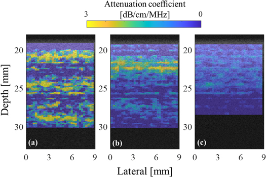
Fig. 8. (Color online) Partial AC overlaid on the B-mode image of the two-layer phantom; the upper layers are (a) 1 mm, (b) 2 mm, and (c) 4 mm.
Download figure:
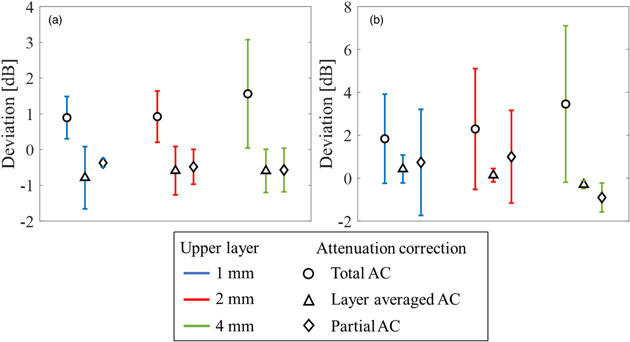
Standard image High-resolution imageIn order to verify the effect of the attenuation compensation, the deviation from the theoretical BSC was calculated. Figure 9 shows the mean value and the SD of the deviation between the measured BSC and the theoretical BSC for each layer with different attenuation corrections. In the upper layer, the maximum deviation using total AC was approximately 3.1 dB, using layer averaged AC was approximately 1.5 dB, and using partial AC calculated in each ROI was approximately 1.2 dB, [Fig. 9(a)]. In particular, stable BSC evaluation can be performed when partial AC is used in the upper layer. The results using local AC were almost the same. On the other hand, in the lower layer, the maximum deviation using total AC was approximately 7.1 dB, using layer averaged AC was approximately 1.0 dB, and using partial AC in each ROI was approximately 3.2 dB, as shown in Fig. 9(b). Therefore, it can be said that BSC evaluation in areas where sufficient sound pressure is not applied or in tissues with complex structures should use average AC in a relatively large area rather than AC calculated from extremely small ROI.
Fig. 9. (Color online) Mean and standard deviation of deviation between the measured and theoretical BSC in each layer with different attenuation corrections; (a) the upper layer and (b) the lower layer.
Download figure:
Standard image High-resolution image
4. Conclusions
In order to improve the accuracy of BSC evaluation of living tissues having layered structures with significantly different properties such as skin, the effect of attenuation correction was verified using an annular array transducer and self-made phantoms. When there is a layer with strong scattering on the surface of the tissue where ultrasonic waves are incident, the evaluation accuracy of the deep area (lower layer) fluctuates depending on the thickness of the surface (upper) layer. The best way to improve the evaluation accuracy in the deep area was to use the average attenuation of only the evaluation region instead of using the average attenuation of the entire evaluation target medium for correction, which is a general method. A method using partial attenuation was also evaluated, however, it did not sufficiently cancel the characteristics of the sound field and had an excessive effect on the evaluation of BSC. In future studies, BSC assessment will be performed on in vivo skin tissue which has a more complex structure.
Acknowledgments
This work was partly supported by JSPS Core-to-Core Program JSPSCCA20170004, and KAKENHI Grant Numbers 19H04482, the Institute for Global Prominent Research at Chiba University, and National Institutes of Health Grant Number EB022950.