Abstract
This article introduces a lumped electrochemical model for lithium-ion batteries. The governing equations of the standard 'pseudo 2-dimensional' (p2D) model are volume-averaged over each region in a cathode-separator-anode representation. This gives a set of equations in which the evolution of each averaged variable is expressed as an overall balance containing internal source terms and interfacial fluxes. These quantities are approximated to ensure mass and charge conservation. The averaged porous domains may thus be regarded as three 'tanks-in-series'. Predictions from the resulting equation system are compared against the p2D model and simpler Single Particle Model (SPM). The Tanks-in-Series model achieves substantial agreement with the p2D model for cell voltage, with error metrics of <15 mV even at rates beyond the predictive capability of SPM. Predictions of electrochemical variables are examined to study the effect of approximations on cell-level predictions. The Tanks-in-Series model is a substantially smaller equation system, enabling solution times of a few milliseconds and indicating potential for deployment in real-time applications. The methodology discussed herein is generalizable to any model based on conservation laws, enabling the generation of reduced-order models for different battery types. This can potentially facilitate Battery Management Systems for various current and next-generation batteries.
Export citation and abstract BibTeX RIS

This is an open access article distributed under the terms of the Creative Commons Attribution Non-Commercial No Derivatives 4.0 License (CC BY-NC-ND, http://creativecommons.org/licenses/by-nc-nd/4.0/), which permits non-commercial reuse, distribution, and reproduction in any medium, provided the original work is not changed in any way and is properly cited. For permission for commercial reuse, please email: oa@electrochem.org.
Lithium-ion batteries are achieving increasing ubiquity with the emphasis on renewable energy and electric transportation to address greenhouse gas pollution. Material and manufacturing innovations, coupled with market pressures and economies of scale, have led to declines in battery pack costs of nearly 85% in the period 2010–18.1 An important factor toward enabling further reductions in cost metrics is the efficient operation of battery systems. This entails maximizing utilization, reducing overdesign, enabling fast charging, and mitigating degradation phenomena. Thermal runaway and the resulting likelihood of fires and explosions is another critical consideration, and it is essential to ensure battery operation in the safe temperature range. The Battery Management System (BMS) is the combination of hardware and software components that performs the requisite functions to ensure safe and efficient operation.2 An accurate and robust mathematical model is essential for BMS, which estimates battery state variables such as State of Charge (SoC), State of Health (SoH), and temperature.2,3
The incorporation of sophisticated electrochemical models has the potential to enable more powerful and intelligent BMS. In addition to improved prediction of battery states, variables internal to battery electrochemistry allow the formulation of more complete optimization and control problems than would be possible by simple circuit models.4 Achieving this integration requires reduction of the computational demands of complex models, such as the macro-homogeneous 'p2D' models of Newman and co-workers.5 In addition to model reformulation techniques that exploit the underlying mathematical structure of the equations to achieve fast simulation,6,7 the tradeoff between accuracy and computational efficiency has spurred active investigation into simplifications of the p2D model subject to limiting assumptions.8
Since its introduction by Atlung et al.,9 the Single Particle Model (SPM) has been extensively used for efficient simulation, estimation, optimal charging and life-cycle modeling.10–13 The SPM visualizes the electrodes in a lithium-ion battery as two representative spherical particles and considers electrode reactions and transport through the active particle. SPM is particularly attractive since the largest reduction in the number of equations is achieved via simplifications of the solid phase, given that the corresponding equation is solved at each point in the electrode computational grid (see section on Model Development).14,15 Importantly however, it neglects potential and concentration variations in the electrolyte phase, which limits its predictive ability to low-current scenarios and relatively thin electrodes, where liquid phase polarizations can be neglected.8 In addition, SPM assumes a uniform reaction distribution throughout each electrode, which is only attained at moderate currents in which kinetic resistances dominate ohmic effects, and in electrodes which possess a monotonic dependence of equilibrium potential with degree of lithiation.16,17 SPM has been recovered in the limits of fast diffusion dynamics with respect to characteristic discharge time.18 The p2D model also returns SPM in the limit of large changes in characteristic overpotential upon Li intercalation, which results in uniform reaction distributions.19 These limitations have led to efforts to expand the applicability of SPM by introducing simplified descriptions of electrolyte dynamics and non-uniform reaction distributions.
In our past work, we extensively used model reformulation techniques. Millisecond computation times were achieved using coordinate transformation, spectral methods and reformulation enabled by analytical solution,6,14,20,21 and successfully demonstrated in applications for parameter estimation, optimal control, and BMS.10,22,23 Despite detailed analysis and comparisons of efficient simulations of SPM-like models in past work from our group,15 the two and three-parameter models have been arguably the most widely used for control, optimization and BMS by the community at large.14 This motivates the development of efficient models for the electrolyte phase in lithium-ion batteries.
A common approach for the inclusion of non-uniform reaction distributions is to directly assume a polynomial profile for pore-wall flux. Alternatively, polynomial profiles for both electrolyte concentration and potential may be assumed and used to determine the spatial variation of the pore-wall flux.24–26 In addition, some workers have derived closed-form analytical solutions for the pore-wall flux distribution. However, these solutions are only valid under certain assumptions, such as linear kinetics, or by neglecting the diffusional contribution to the electrolyte current, and also neglect the concentration-dependence of one or more electrolyte transport properties.27 Still other approaches assume a polynomial or exponential dependence for the equilibrium electrode potential in space. These assumed profiles are often combined with polynomial spatial dependence for other electrochemical variables, converting the original Partial Differential Equations (PDEs) of the p2D model into a system of Differential Algebraic Equations (DAEs). The simplifications require assumptions to achieve closure, while also assuming constant electrolyte transport properties for tractability.28,29 For both types of approaches, the use of higher-order polynomial profiles for increased accuracy is expected to increase the DAE system size, with the attendant penalty for computational efficiency.
Extensions of SPM to electrolyte dynamics are often termed 'SPMe', where e denotes electrolyte. A common approach begins with the assumption of a uniform reaction in the electrodes.18,20,30 This results in simplified PDEs for electrolyte concentration. For constant electrolyte diffusivity, SPMe results in linear PDEs, which are computationally simple to solve. Indeed, it is possible to derive analytical solutions for the constant diffusivity case.16,31 Alternatively, instead of constant reaction distributions, polynomial spatial dependence for concentration can also be assumed, resulting in a system of DAEs.32–34 With the knowledge of electrolyte concentrations, the electrolyte current equation is usually integrated, or volume-averaged quantities are used to obtain the liquid-phase potential drop. In some cases, polynomial profiles are assumed for the liquid-phase potential as well. This information is then used in conjunction with the electrode-kinetics equation to estimate the cell voltage. The uniform-reaction SPMe20,30 is rigorously derived from the scaled p2D model in the limit of fast electrolyte diffusion dynamics.18 This perturbation approach yields simplified algebraic expressions for the various polarization contributions to the cell voltage. These expressions can be evaluated at negligible computational cost. In addition, the cell voltage equation is expressed in terms of electrode-averaged quantities to obviate the need for assumptions on the pore-wall flux at the terminals.
The PDE system in SPMe becomes non-linear in the case of variable diffusion coefficient, which might compromise computational efficiency. When solving numerically, the non-linearities are likely to entail finer spatial discretization in both the electrode and the solid particle to ensure numerical convergence, which will increase the DAE system size. The stiffness of the resulting system is also likely to increase for the non-linear case, especially at high current densities. The effect of increased computational cost may become more significant in real-time environments, both due to stringent accuracy requirements and hardware limitations.23 In addition, even in situations where the non-linear equation is solved numerically, simplifications of the electrolyte current equation, such as constant electrolyte conductivity,30 are necessary to allow tractable integration for calculating electrolyte ohmic drop. This can be a requirement even if polynomial profiles for electrolyte concentration are assumed for the non-linear equation.35,36 The perturbation approach results in expressions in which the transport properties are evaluated at a given representative concentration.18 This may result in errors in estimating concentration overpotentials at high discharge rates, where substantial spatial variations are expected to arise. Additionally, it is not clear whether the algebraic expressions for electrolyte ohmic drop are valid for variable concentration properties and may have to be rederived. Using a constant value may lead to errors in estimating ohmic drops and concentration overpotentials at high current-densities.
In this article, we use a Tanks-in-Series approach to reduce the p2D model. The electrolyte conservation equations are written in volume-averaged form, without resorting to any direct assumptions on the spatial dependence, unlike in polynomial profile methods. The proposed Tanks-in-Series approach also does not assume uniform reaction rates to predict concentration profiles, since we deal in average quantities. The key approximations are (a) in the interfacial fluxes and (b) using the electrode-averaged pore-wall flux to estimate the electrode-averaged overpotential. The second assumption is analogous to some SPMe models.18 For problem closure, we make reasonable approximations for the flux variables at the interface. Mass and charge conservation are imposed at the domain interfaces in order to determine the unknown interfacial values. The cell-voltage is then calculated from the known electrode-averaged pore-wall flux. This formulation allows for the inclusion of concentration-dependent transport properties, since terminal-to-terminal integration is not required, and the properties are only evaluated at the domain interfaces. In addition, it reduces the full p2D model into a fixed-size system of < 20 DAEs and no PDEs need be solved.
The article is structured as follows. We first illustrate the systematic development of the Tanks-in-Series model from the full p2D model. This is followed by a short description of the computational details of the simulations and the parameters used therein. Simulation results are then presented that illustrate the voltage-time discharge curves, electrolyte phase predictions, and the qualitative and quantitative features of the model as a function of discharge rate. The validity of the flux approximations is then examined for an aggressive case of ultra-thick electrodes with severe electrolyte diffusion limitations, followed by a representative comparison of the Tank Model with a version of the SPMe for variable transport properties. Computational time benchmarks are presented against standard implementations of the p2D model to quantify the computational speed. The article concludes with a short discussion on parameter estimation and other applications, extensions to different battery systems, and assessments against other reduced-order models.
Model Development
The pseudo 2-dimensional (p2D) model of Newman and co-workers is a continuum electrochemical model that has found substantial application for simulation of Li-ion battery performance.10 Figure 1 illustrates the computational schematic of the model.5,17 The typical p2D model is written for a single 'cathode-separator-anode' sandwich. Each domain is modeled using porous electrode theory, in which the two solid and electrolyte phases are regarded as superimposed continua.37 The model is a set of coupled partial differential equations (PDEs) based on one-dimensional conservation laws for charge and mass in each domain. The individual domain equations are coupled through the specification of appropriate interfacial boundary conditions, which also ensure mathematical well-posedness. In the p2D representation of the battery, the active material is regarded as composed of spherical particles of uniform radii. Lithium intercalation and de-intercalation occurs through electron-transfer reactions at the particle surface and transport through the solid particle, modeled by conservation laws in the 'pseudo' r-dimension. The complete mathematical model and parameter values may be found in Tables I–III.
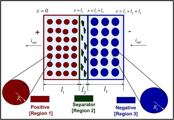
Figure 1. Schematic representation of the computational domain in the p2D model for a dual insertion lithium-ion cell. The active material in both electrodes is modeled as spherical particles. Electron-transfer reactions are modeled at the particle-electrolyte interface, as is the transport of intercalated lithium through the active particle. Liquid phase mass and charge transport through the thickness li of each domain also modeled using concentrated solution theory. Electron transport through the solid phase is also considered, with electronic current entering and leaving the cell at the current collectors (not shown). The color codes for the three porous domains are used throughout this article, i.e. dark red (positive electrode), dark green (separator), and dark blue (negative electrode).
Table I. Governing PDEs for the p2D model.
| Equations | Boundary Conditions |
|---|---|
| Positive Electrode (Region 1) | |
 |
 |
 |
 |
 |
 |
 |
 |
| Separator (Region 2) | |
 |
 |
 |
 |
| Negative Electrode (Region 3) | |
 |
 |
 |
 |
 |
 |
 |
 |
Table III. Base case model parameters (constant values).
| Symbol | Parameter | Negative Electrode | Separator | Positive Electrode | Units |
|---|---|---|---|---|---|
| εi | Porosity | 0.3 | 0.4 | 0.3 | |
| εfi | Electrode filler fraction | 0.038 | 0.12 | ||
| bi | Brugemann tortuosity correction | 1.5 | 1.5 | 1.5 | |
| ai | Particle surface area per unit volume | 1740000 | 1986000 | m2/m3 | |
| cis, max | Maximum particle phase concentration | 31080 | 51830 | mol/m3 | |
| cis, 0 | Initial particle phase concentration | 24578 | 18645 | mol/m3 | |
| c0 | Initial electrolyte concentration | 1200 | mol/m3 | ||
| Dsi | Solid phase diffusivity | 1.4 × 10⁻¹⁴ | 2.0 × 10⁻¹⁴ | m2/s | |
| ki | Electrode reaction rate constant | 6.626 × 10⁻¹⁰ | 2.405 × 10⁻¹⁰ | m2.5/(mol0.5s) | |
| αa, i | Electrode reaction anodic coefficient | 0.5 | 0.5 | ||
| αc, i | Electrode reaction cathodic coefficient | 0.5 | 0.5 | ||
| li | Electrode thickness | 40 × 10−6 | 25 × 10−6 | 36.55 × 10⁻⁶ | m |
| Ri | Characteristic particle radius | 10−6 | 10−6 | m | |
| t0+ | Li+ transference number | 0.38 | |||
| σi | Electronic conductivity | 100 | 100 | S/m | |
| T | Temperature | 298.15 | K | ||
| iapp | Current Density (1C) | -17.54 | A/m2 | ||
In deriving the Tanks-in-Series model, the volume-averaging procedure is applied first to the solid phase conservation equations, illustrating how SPM is recovered under certain assumptions. The concept is then applied to the electrolyte transport equations, thereby resulting in averaged equations for the liquid phase 'Tanks' of Figure 2.
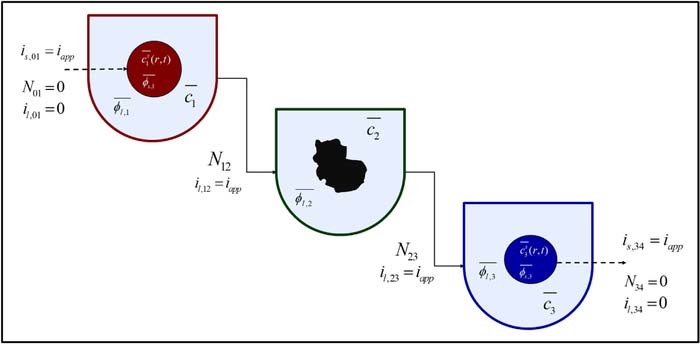
Figure 2. A visualization of the Tank Model approach depicting the mass and charge flows in to and out of each 'tank'. Since both the electrolyte flux and liquid phase current density are zero at the current collectors, net flows into the liquid phase of the positive 'tank' and out of the negative 'tank' are zero. The interfacial boundary conditions at the separator define the mass and charge flows for the middle separator 'tank'. The electronic current carried by the solid phase at the current collectors is denoted by dotted lines. The solid and liquid phases exchange mass and charge at a rate determined by the pore-wall flux  , an internal exchange which is not shown here. The sign convention is so adopted that iapp is negative during discharge.
Solid particle transport
In the absence of complexities such as phase-separation or concentrated solution effects,38,39 solid phase transport is modeled by Fick's second law in spherical coordinates. For the positive electrode particle, we have
![Equation ([1])](https://content.cld.iop.org/journals/1945-7111/167/1/013534/revision1/d0001.gif)
Where the r coordinate denotes the radial distance within the particle and is thus the second 'pseudo-dimension'. The subscript 1 denotes variables and parameters pertinent to the positive electrode (region 1).
In porous electrode theory, Equation 1 is valid at each point along the electrode thickness x. The superscript s is used to denote the solid phase. Ds1 is the diffusion coefficient in the positive particle. The second-order problem in r requires the specification of two boundary conditions. At the surface of the solid particle, the diffusive flux is related to the local rate of electrode reaction, or the pore-wall flux as
![Equation ([2])](https://content.cld.iop.org/journals/1945-7111/167/1/013534/revision1/d0002.gif)
A symmetry boundary condition is applied at the center of the positive particle
![Equation ([3])](https://content.cld.iop.org/journals/1945-7111/167/1/013534/revision1/d0003.gif)
The analogous set of equations are written for the negative electrode (region 3)
![Equation ([4])](https://content.cld.iop.org/journals/1945-7111/167/1/013534/revision1/d0004.gif)
With the boundary conditions given by
![Equation ([5])](https://content.cld.iop.org/journals/1945-7111/167/1/013534/revision1/d0005.gif)
![Equation ([6])](https://content.cld.iop.org/journals/1945-7111/167/1/013534/revision1/d0006.gif)
The Butler-Volmer equation is a common constitutive relation for the pore-wall flux in each electrode as follows
![Equation ([7])](https://content.cld.iop.org/journals/1945-7111/167/1/013534/revision1/d0007.gif)
Where k1 is the rate constant for the positive electrode reaction, and cs, max 1 denotes the maximum concentration of Li in the positive electrode particle. F and R denote Faraday's constant and the gas constant respectively. α's are the charge transfer coefficients for each electrode reaction. The quantity η = ϕs, 1 − ϕl, 1 − U1(cs.surf1) is the surface overpotential, expressed as the difference between the solid and liquid phase potentials minus the electrode open circuit potential U1(cs, surf1) vs. a Li/Li+ reference electrode. cs, surf1 is the solid particle concentration evaluated at the surface of the particle, i.e.
![Equation ([8])](https://content.cld.iop.org/journals/1945-7111/167/1/013534/revision1/d0008.gif)
The dependence of open circuit potential (OCP) on the surface concentration is indicated accordingly. The equivalent expression for the negative electrode is given by
![Equation ([9])](https://content.cld.iop.org/journals/1945-7111/167/1/013534/revision1/d0009.gif)
Equations 1 and 4 can be volume-averaged over their respective electrode volumes. For the positive electrode, we obtain
![Equation ([10])](https://content.cld.iop.org/journals/1945-7111/167/1/013534/revision1/d0010.gif)
The volume-averaged form becomes
![Equation ([11])](https://content.cld.iop.org/journals/1945-7111/167/1/013534/revision1/d0011.gif)
Similarly, for the negative electrode, we have
![Equation ([12])](https://content.cld.iop.org/journals/1945-7111/167/1/013534/revision1/d0012.gif)
The corresponding boundary conditions can also be expressed in volume-averaged form.
![Equation ([13])](https://content.cld.iop.org/journals/1945-7111/167/1/013534/revision1/d0013.gif)
Numerical solution of these equations entails spatial discretization in the spherical dimension. Discretization of Equations 11 and 12 results in a system of Differential Algebraic Equations (DAEs), with a convenient linear form for constant Dsi. For discretization, we employ an efficient three-parameter model based on a biquadratic profile for the radial dependence of csi.14,40 This approximation is expected to ensure higher accuracy than a two-parameter parabolic profile even at relatively high rates of discharge. The discretized system of equations is therefore
![Equation ([14])](https://content.cld.iop.org/journals/1945-7111/167/1/013534/revision1/d0014.gif)
![Equation ([15])](https://content.cld.iop.org/journals/1945-7111/167/1/013534/revision1/d0015.gif)
![Equation ([16])](https://content.cld.iop.org/journals/1945-7111/167/1/013534/revision1/d0016.gif)
Where the three-parameter model has been expressed in terms of the particle-averaged solid phase concentration  , the particle-averaged concentration gradient
  , and the particle surface concentration
  . The particle average concentrations are related to the State of Charge (SoC) at the cell level and is directly obtained from the simulation results in the above formulation.
As mentioned earlier, the focus of this article is the development of efficient equations for the electrolyte phase, and therefore the most commonly adopted solid-phase approximation is used in this article. While other reformulation and approximation techniques may be more suitable at higher discharge rates and parameter combinations, we chose this approximation to (a) explain the concepts with a simpler approximation for brevity and easier adoption of current work (b) to alert users the importance of more detailed and relevant approximations published elsewhere.15 Importantly, the accuracy of the quartic profile approximation was quantitatively verified against nearly error-free numerical methods (collocation, finite difference) for the cases considered in this article.
Solid phase charge transport
For charge transport in the solid phase, the governing equation may be written as a conservation law for charge as follows37,41
![Equation ([17])](https://content.cld.iop.org/journals/1945-7111/167/1/013534/revision1/d0017.gif)
The time-derivative for charge density is ignored due to electroneutrality.
Similarly, we have, for the negative electrode
![Equation ([18])](https://content.cld.iop.org/journals/1945-7111/167/1/013534/revision1/d0018.gif)
Here, are is, 1 and is, 3 denote the solid phase current densities. The constitutive equation for the solid phase current density is an Ohm's law expression based on the effective electronic conductivity and local potential gradient as follows
![Equation ([19])](https://content.cld.iop.org/journals/1945-7111/167/1/013534/revision1/d0019.gif)
Where 1 − εi − εf, i is the fraction of solid phase in electrode i, after subtracting the liquid and inert volume fractions. This factor corrects for the actual conduction pathways in the electrode material. More detailed correction factors may also be applied. The solid phase volume fraction also appears in the specific interfacial area, which for perfectly spherical particles is given by  .
.
Volume-averaging gives us
![Equation ([20])](https://content.cld.iop.org/journals/1945-7111/167/1/013534/revision1/d0020.gif)
Using the boundary conditions that impose the solid phase current density at the interfaces, one can simplify Equation 20 as
![Equation ([21])](https://content.cld.iop.org/journals/1945-7111/167/1/013534/revision1/d0021.gif)
Volume averaging thus connects the applied cell current density iapp and average pore-wall flux. The sign convention for the model is so adopted that iapp is negative during discharge.
![Equation ([22])](https://content.cld.iop.org/journals/1945-7111/167/1/013534/revision1/d0022.gif)
Similarly, for the negative electrode, we have
![Equation ([23])](https://content.cld.iop.org/journals/1945-7111/167/1/013534/revision1/d0023.gif)
Equations 21 and 22 can be used in conjunction with the volume - averaged forms of Equations 1–6 to determine the temporal evolution of average solid-phase concentrations for a given iapp. In effect, the active material in each electrode is now modeled by a single representative particle,18 the Li concentration profiles through which will be influenced by factors such as the applied current density iapp, solid phase diffusion coefficients Dsi and the characteristic particle radius Ri. This set of equations also determines the evolution of the averaged surface particle concentration, which in turn affects the surface overpotentials and thus the cell voltage response through constitutive Equations 7 and 9. These equations are volume-averaged in order to obtain a relationship between the average pore-wall fluxes  and the average potentials
  and
and  . This is illustrated for the positive electrode in Equation 24 below
![Equation ([24])](https://content.cld.iop.org/journals/1945-7111/167/1/013534/revision1/d0024.gif)
Unlike the equations for electrolyte concentration, the highly non-linear nature of the constitutive equation renders evaluation of Equation 24 cumbersome and likely impossible without the use of a full-order solution that gives the actual spatial dependence of the variables. To this end, averages of non-linear quantities are approximated by their value at the average values of the variables on which they depend (i.e.  ).
).
Mathematically, this can be stated as
![Equation ([25])](https://content.cld.iop.org/journals/1945-7111/167/1/013534/revision1/d0025.gif)
The classic Single Particle Model (SPM) employs an additional simplification by ignoring the dynamics of the electrolyte phase. Therefore,  , implying that the electrolyte concentration is always equal to its initial value. Neglecting liquid phase variations also means that
  is often set to a constant reference, e.g.
  for all i.
Neglect of ohmic and electrolyte concentration effects restricts the accuracy of SPM to operating regimes characterized by low ohmic losses, low currents, and kinetically limited electrodes, which usually result in spatially uniform pore-wall flux distributions.16,30 To this end, the Tanks-in-Series descriptions of electrolyte dynamics are expected to augment and improve the practical applicability of SPM.
Electrolyte mass balance: volume-averaging
We begin with the governing equation for electrolyte concentration for an isothermal model in one spatial dimension. The equations for c based on porous electrode theory may be expressed in the form of conservation laws37
In the positive electrode,
![Equation ([26])](https://content.cld.iop.org/journals/1945-7111/167/1/013534/revision1/d0026.gif)
Due to the absence of solid active material, the conservation equation for c in the separator is characterized by a lack of a source term as
![Equation ([27])](https://content.cld.iop.org/journals/1945-7111/167/1/013534/revision1/d0027.gif)
The subscript 2 is used to denote the variables in the separator domain.
The equation for the negative electrode is identical in form to that of the positive electrode
![Equation ([28])](https://content.cld.iop.org/journals/1945-7111/167/1/013534/revision1/d0028.gif)
N1, N2, N3 may regarded as electrolyte fluxes, which need to be related to local concentration gradients. Noting the similarity of the governing equations to Fick's second law, we have the following constitutive equations41
![Equation ([29])](https://content.cld.iop.org/journals/1945-7111/167/1/013534/revision1/d0029.gif)
In the above equations, D(c) denotes the concentration-dependent electrolyte diffusion coefficient, corrected by a Bruggemann-type factor to account for porous medium tortuosity.
The governing equations for electrolyte concentration are second-order in space, which entails the specification of two boundary conditions for c1, c2 and c3. The boundary conditions are defined at the extremities of each domain. The positive and negative current collectors are physical barriers to the transport of Li+ ions, and thus the electrolyte flux at these locations is set to zero. These boundary conditions are thus given by
![Equation ([30])](https://content.cld.iop.org/journals/1945-7111/167/1/013534/revision1/d0030.gif)
And,
![Equation ([31])](https://content.cld.iop.org/journals/1945-7111/167/1/013534/revision1/d0031.gif)
In addition, electrolyte concentrations and their fluxes must be continuous at the interface between the separator and electrodes. At the positive electrode-separator interface, this is expressed as
![Equation ([32])](https://content.cld.iop.org/journals/1945-7111/167/1/013534/revision1/d0032.gif)
In general Nij is used to denote the flux at the interface of regions i and j.
Similarly, at the interface between the separator and negative electrode, we have
![Equation ([33])](https://content.cld.iop.org/journals/1945-7111/167/1/013534/revision1/d0033.gif)
Now, Equation 26 is integrated over the volume of the positive electrode V1 as
![Equation ([34])](https://content.cld.iop.org/journals/1945-7111/167/1/013534/revision1/d0034.gif)
For the one-dimensional model in cartesian coordinates, the differential volume dV is given by dV = Adx, where A is a constant that may be considered a cross-sectional area. In addition, we express the integrals in terms of average quantities as  , and
, and  , with
  denoting the volume average of variable v in a given 'tank'. Substituting these relations converts the volume integral into a one-dimensional integral over electrode thickness, i.e. from x = 0 to x = l1.
Equation 34 thus becomes
![Equation ([35])](https://content.cld.iop.org/journals/1945-7111/167/1/013534/revision1/d0035.gif)
Here, we make the reasonable assumption that the electrode porosity ε1, specific interfacial area a1 and Li+ transport number t0+ in the electrolyte phase are constant in both space and time.42
Using Equation 30, Equation 35 reduces to
![Equation ([36])](https://content.cld.iop.org/journals/1945-7111/167/1/013534/revision1/d0036.gif)
The same sequence of operations gives us the volume-averaged equations for the separator and negative electrode as follows
![Equation ([37])](https://content.cld.iop.org/journals/1945-7111/167/1/013534/revision1/d0037.gif)
![Equation ([38])](https://content.cld.iop.org/journals/1945-7111/167/1/013534/revision1/d0038.gif)
It is worth noting that the steps applied so far represent a rigorous volume-averaging of the equations in each porous domain, followed by the use of the boundary conditions to eliminate interfacial flux terms where possible. No approximations have been made up to this point.
Electrolyte mass balance: approximating fluxes
In order to track the average concentrations in each 'tank', we begin with the volume-averaged concentration Equations 36–38. Inspection of these equations reveals the presence of the unknown interfacial flux terms that require suitable approximations to achieve closure. In doing so, we can exploit the flux boundary conditions 32 and 33, which establish the mass flow coupling between adjacent tanks in series.
A simple approximation for the interfacial diffusive flux is in terms of a 'driving force' Δc and a 'length scale' approximation δi, ij within domain i for the interface between domains i and j. The concept is depicted in Figure 3. This is analogous to the 'diffusion-length' approach attempted previously, but we dispense with assumptions on the spatial profiles for c.32,43 The 'driving force' Δc is expressed in terms of a difference between the average concentration and the unknown interfacial concentration  , and we use
  as a first approximation. We therefore have, using the constitutive Equations 29
![Equation ([39])](https://content.cld.iop.org/journals/1945-7111/167/1/013534/revision1/d0039.gif)
On the separator side of the interface, we assume  , which we use for the flux approximation
![Equation ([40])](https://content.cld.iop.org/journals/1945-7111/167/1/013534/revision1/d0040.gif)
An equivalent interpretation of the above flux approximations is that we have assumed that the concentration at the midpoint of the porous domain equal to the volume average. This approximation is mathematically equivalent to Gaussian integration with one point, accurate to l21.
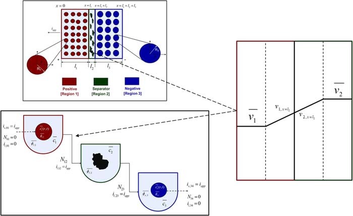
Figure 3. Representing the flux approximations at the interface of two regions. The example is illustrated for the positive electrode-separator interface.
Substitution of the above approximations into the continuity conditions of Equations 32 gives us
![Equation ([41])](https://content.cld.iop.org/journals/1945-7111/167/1/013534/revision1/d0041.gif)
The interfacial concentration is now expressed in terms of tank averages as
![Equation ([42])](https://content.cld.iop.org/journals/1945-7111/167/1/013534/revision1/d0042.gif)
In general, we use the notation vij to denote the value of a given variable v at the interface of domains i and j. An identical sequence of steps yields the concentration at the separator-negative interface as
![Equation ([43])](https://content.cld.iop.org/journals/1945-7111/167/1/013534/revision1/d0043.gif)
Substituting the values of interfacial concentrations back into the flux approximations allows us to express the interfacial fluxes in terms of tank-average variables. Thus, we have
![Equation ([44])](https://content.cld.iop.org/journals/1945-7111/167/1/013534/revision1/d0044.gif)
![Equation ([45])](https://content.cld.iop.org/journals/1945-7111/167/1/013534/revision1/d0045.gif)
Equations 44 and 45 can thus be inserted into the volume-averaged forms 36–38 to obtain a system of Ordinary Differential Equations (ODEs). It is important to equate the approximations for the total flux, and not just the driving forces.44 This ensures true mass conservation.
In the three 'tanks', after substituting the known values of average pore-wall fluxes, we have
![Equation ([46])](https://content.cld.iop.org/journals/1945-7111/167/1/013534/revision1/d0046.gif)
![Equation ([47])](https://content.cld.iop.org/journals/1945-7111/167/1/013534/revision1/d0047.gif)
![Equation ([48])](https://content.cld.iop.org/journals/1945-7111/167/1/013534/revision1/d0048.gif)
As specified previously, a slight difference between this approach and others in literature18,30,36,45 is that it avoids the assumption of uniform reaction rate (given by the pore-wall flux) to solve the PDEs for concentration, but instead deals in average quantities. This allows the prediction of average concentration trends even when the constant pore-wall flux assumption is not applicable, with the flux approximations as the sole source of error. Inspection of Equations 46–48 also suggests their decoupling from those for other electrochemical variables, indicating that they may be solved independently as an ODE system, the solutions of which may be used to compute other relevant quantities during post-processing. While all model equations are simulated simultaneously throughout this article, such a segregated approach may be computationally efficient in real-time control or resource-constrained environments and is enabled by the Tanks-in-Series model. Leaving the model in this form allows for the incorporation of nonlinear diffusivities.
Liquid phase charge transport
The governing equation for electrolyte current is related to charge conservation in the electrolyte phase. Thus, we have
![Equation ([49])](https://content.cld.iop.org/journals/1945-7111/167/1/013534/revision1/d0049.gif)
Where the constitutive equation for electrolyte current is given by a modified Ohm's law based on concentrated solution theory. Thus
![Equation ([50])](https://content.cld.iop.org/journals/1945-7111/167/1/013534/revision1/d0050.gif)
The concentration-dependent ionic conductivity κ(c) is corrected by a tortuosity factor specific to each region.
Now, volume-averaging Equation 49 is redundant, ultimately resulting in Equation 21 due to the overall charge balance imposed by porous electrode theory. However, the interfacial boundary conditions for i2, i provide for the estimation of liquid phase ohmic effects. At the interface between the electrodes and separator, the entire current iapp is carried by the liquid phase, and the solid-phase current density is zero. Using the constitutive Equation 50, we therefore have, at the positive electrode-separator interface
![Equation ([51])](https://content.cld.iop.org/journals/1945-7111/167/1/013534/revision1/d0051.gif)
Where we have defined the thermodynamic factor as  . The tank-averaged equations for the electrolyte potential are now written as
![Equation ([52])](https://content.cld.iop.org/journals/1945-7111/167/1/013534/revision1/d0052.gif)
Where an approximation  and
and  , analogous to Equations 39 and 40 is made for the gradients of ϕl, i, in terms of tank-average and interfacial values. Equating the interfacial current density results in Equation 53, which can be solved in conjunction with continuity conditions to obtain the interfacial electrolyte potential.
![Equation ([53])](https://content.cld.iop.org/journals/1945-7111/167/1/013534/revision1/d0053.gif)
Solving for ϕl, 12 gives us
![Equation ([54])](https://content.cld.iop.org/journals/1945-7111/167/1/013534/revision1/d0054.gif)
A similar form is obtained at the separator-negative electrode interface
![Equation ([55])](https://content.cld.iop.org/journals/1945-7111/167/1/013534/revision1/d0055.gif)
Equations 39–43 can now be combined with Equations 51–55 to give us the algebraic equations governing electrolyte potential
![Equation ([56])](https://content.cld.iop.org/journals/1945-7111/167/1/013534/revision1/d0056.gif)
The final step in the model formulation is the specification of a reference potential. A convenient reference is the electrolyte potential at the interface between the separator and positive electrode. We thus set ϕl, 12 = 0. This modifies Equation 54, and completes the DAE system for the Tank Model.
![Equation ([57])](https://content.cld.iop.org/journals/1945-7111/167/1/013534/revision1/d0057.gif)
We can now assemble the complete Tanks-in-Series Model in Table IV.
Table IV. Governing Equations of the Tanks-in-Series Model.
| Positive Electrode (Region 1) | Separator (Region 2) | Negative Electrode (Region 3) |
|---|---|---|
 |
 |
 |
 |
 |
 |
 |
 |
|
 |
 |
|
 |
 |
|
  |
  |
Cell voltage
Solving the system of Table IV now allows the prediction of the cell voltage as
![Equation ([58])](https://content.cld.iop.org/journals/1945-7111/167/1/013534/revision1/d0058.gif)
In using Equation 58 to calculate cell voltage for the Tanks-in-Series Model, it is implicitly assumed that the solid phase potentials at the cell termini may be approximated by their respective electrode averages. In reality, the terminal potentials must be determined via interfacial approximations for the constitutive Equations 19 analogous to Equations 52 for ϕl, i. Accounting for this potential drop may be necessitated at high current densities, or for electrodes with poor electronic conductivity. In practice, σeff ∼ 50 S/m and the ϕs, i gradients within the electrode are negligible. This can be seen by the following rough estimation for an aggressive |iapp| = 100 A/m2 and σeff = 1 S/m, and electrode thickness l1 = 100μm. We therefore have
![Equation ([59])](https://content.cld.iop.org/journals/1945-7111/167/1/013534/revision1/d0059.gif)
Thus, the upper limit of this solid phase ohmic drop is ∼5 mV per electrode. This justifies the assumption of uniform ϕs, i for most situations of practical salience.
Model Parameters
Table III lists the parameter values for a 1.78 Ah Nickel-Cobalt-Manganese (NCM)/graphite power cell, collated from various sources by Tanim et al.33 Electrolyte transport property correlations were taken from the work of Valøen and Reimers, and are listed in Table II.42 A modified value of Ri = 1 μm was used for the particle radii, in order to ensure rapid diffusion with negligible gradients. The absence of solid phase diffusion limitations serves the practical purpose of ensuring the accuracy of our three-parameter model for solid phase transport even at relatively high discharge rates, based on the quantitative guidelines of Subramanian et al.40 This prevents numerical errors for solid phase discretization from confounding our analysis, which is focused on examining the accuracy of our Tanks-in-Series equations for the liquid phase.
Table II. Additional constitutive equation.
 |
 |
 |
| σeff, i = σi(1 − εi − εf, i), i ∈ {1, 3} |
 |
 |
 |
 |
 |
 |
 |
Computational Details
The full p2D model is used as the benchmark in evaluating the predictions of the Tanks-in-Series model. The p2D model was discretized and solved using coordinate transformation, model reformulation and orthogonal collocation techniques described in previous work.6 The number of collocation points in each region were adjusted to achieve numerical convergence of discharge curves at different current densities, ultimately selecting n = (7,3,7) Gauss-Legendre collocation points. Comparisons of the Tank Model with SPM are also reported, for which a Finite-Difference discretization with n = 256 internal node points were employed. All DAE systems were consistently initialized,46 and solved using the dsolve function in Maple 2018.47 An absolute solver tolerance abserr = 10− 8 was specified.
For evaluating computational performance, the discretized equations were solved in time using IDA, an Implicit Differential-Algebraic solver in ANSI-standard C language under BSD license. IDA is an efficient solver for initial value problems (IVP) for systems of DAEs, which is part of the SUNDIALS (SUite of Nonlinear and DIfferential/ALgebraic equation Solvers) package.48 The absolute solver tolerance was set to atol = 10− 8 and a relative tolerance of rtol = 10− 7 was specified.
All computations were performed on an Intel Core i7-7700K processor with a clock speed of 4.2 GHz, 8 logical cores and 64 GB RAM.
Results and Discussion
Base case model comparisons
In this section, the Tanks-in-Series model is simulated for galvanostatic discharge at C-rates of 1C, 2C, and 5C. In comparing the model predictions to the full p2D model, we seek to ascertain the accuracy of the Tanks-in-Series approximations, and to quantify its deviation from p2D as a function of applied current density. The results are also compared against curves from SPM, chiefly to illustrate improvement over commonly used fast physics-based models.
Galvanostatic discharge curves
Figure 4 compares the cell voltage-time predictions of our Tanks-in-Series model (hereafter termed the 'Tank Model') with SPM and the full p2D model. The agreement of all three models at 1C and 2C indicates relatively low liquid phase polarizations compared to other overpotentials, possibly due to the values of the Base Case parameters, which are those of a power-cell rated for higher discharge rates. Even so, there is a discernible improvement with the Tank Model. The improved accuracy of the tank model at 5C discharge is substantially more pronounced, particularly during the intermediate phase of the discharge process. This is further illustrated in Figure 5, which depicts the instantaneous error for Vcell. The qualitative trends are identical for both the Tank Model and SPM, but the curves for the Tank Model appear shifted by nearly a constant value compared to SPM. This difference is due to the Tank Model's estimates of liquid phase ohmic drops and concentration overpotentials, which reduces error. The magnitude of these overpotentials increases with current density as characterized by the C-rate.
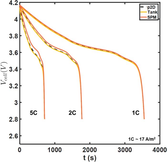
Figure 4. Model comparisons for cell voltage at different rates of discharge. The tank model (gold) coincides almost exactly with the p2D model, obscuring the black dashed curves of the latter. This color code is used throughout the article in all model comparisons involving SPM.
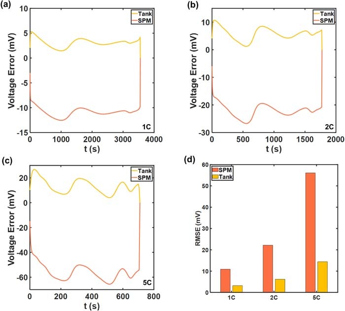
Figure 5. Instantaneous voltage errors with respect to the p2D model at (a) 1C (b) 2C (c) 5C discharge. (d) compares the overall Root Mean Square Errors (RMSE). The error profiles exhibit oscillations.
The increased accuracy of the Tank Model at 5C is illustrated in Figures 5c, and 5d, with the absolute error only slightly exceeding 20 mV, in contrast to >60 mV for SPM. A more than threefold reduction in RMSE is obtained at 5C due to the incorporation of the lumped equations for the electrolyte.
The oscillatory instantaneous error profiles in Figure 5 can be observed in other reduced-order models.18,25,26 The maximum amplitude of the oscillations, corresponding to the maximum absolute error, expectedly increases with discharge rates. Sources of this error may be in the liquid phase approximations of the Tank Model, and in the estimation of electrode averaged overpotential from the electrode averaged current as in Equation 25. In this case, the contribution of errors from the solid phase concentration is expected to be negligible given the choice of particle size Ri, which ensures rapid diffusion dynamics and attainment of steady state in ∼50 s. This can also be seen in Figure 6, in which the averaged particle surface concentrations  across the three models at 1C are compared. The close agreement of the Tank Model to the finely discretized SPM and p2D models indicates the accuracy of the biquadratic profile approximations 14–16. Even at a higher current density of 5C, agreement is ensured in both electrode particles, as depicted in Figure 7. However, the average values may still obscure variations across the electrode thickness due to a non-uniform reaction distribution. In particular, the particle surface concentration at the termini will also deviate from its electrode average due to variations in local pore-wall flux ji. Such deviation from the average values of Equations 22 and 23 results in errors in reaction overpotentials, which contributes to errors in Vcell.
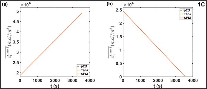
Figure 6. Comparison of electrode-averaged particle surface concentrations at 1C discharge for (a) positive electrode and (b) negative electrode. The close agreement between the three models means the curves are nearly on top of each other.
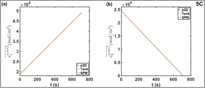
Figure 7. Comparison of electrode-averaged particle surface concentrations at 5C discharge rate for (a) positive electrode and (b) negative electrode. The close agreement between the three models means the curves are nearly on top of each other.
Figure 8 compares the spatial distribution of pore-wall fluxes at 1C. The positive electrodej1 achieves rapid uniformity, even though the reaction is initially confined near the separator interface at t = 0. Minor oscillations and deviations from the average are observed toward the end of discharge, but the relative change is negligible compared to that for the negative electrode j3. The local value near the separator is six times higher than the Tank Model average at the beginning of the discharge, whereas j3 ∼ 0 near the negative collector. The maxima shift toward the negative collector as the discharge progresses. The reaction 'front' propagates through the electrode, and successive peaks are observed at the two points. Throughout the discharge, the local intercalation rate near the terminal deviates substantially from the Tank Model, sometimes by a factor of two, approaching the average  only toward the end of discharge. The reaction distribution in a porous electrode is the result of the relative balance between reaction kinetics, ohmic resistances, and the functional dependence of the open circuit potential U(cs, surfi). Non-uniform reaction distributions are observed in electrodes with faster kinetics with respect to ionic or electronic transport, and flat OCP curves.17,49 The U(cs, surfi) curve for graphite has a substantially flat section corresponding to multiple phase transitions at different degrees of lithiation.50 In contrast, U(cs, surfi) for the NCM positive electrode exhibits a more monotonic dependence with a larger (in magnitude) average slope over the full lithiation range. The non-uniform reaction distribution thus contributes to the error in the Tank Model, in addition to the approximations for liquid phase.19 These effects are even more pronounced in Figure 9, which examines these trends at 5C. The larger relative deviation close to the negative collector is expected at the higher overall current density. Additionally, oscillatory trends are also observed for the positive electrode beyond t ∼ 300 s, with the deviations about the average increasing to ∼20%.
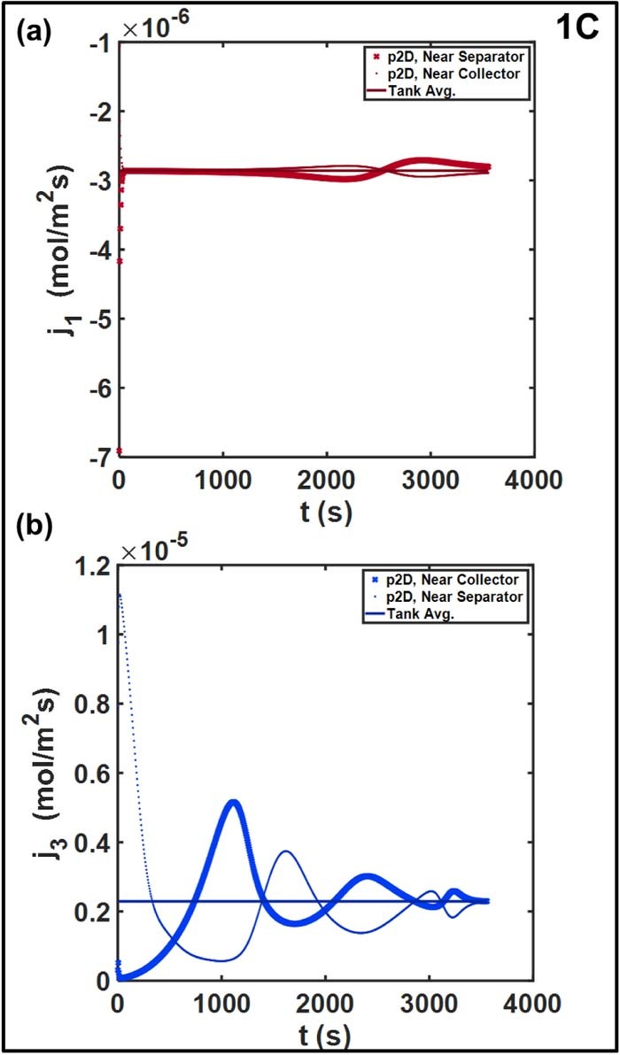
Figure 8. Spatial distribution of pore-wall flux in (a) positive electrode and (b) negative electrode at 1C. The error due to the use of the average pore-wall flux to estimate the cell voltage is expected to be larger in magnitude for the spike-shaped profile for the negative electrode.
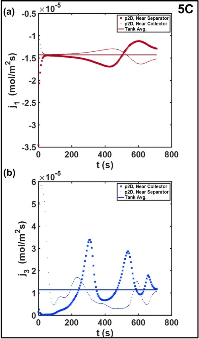
Figure 9. Spatial distribution of pore-wall flux in (a) positive electrode and (b) negative electrode at 5C . The non-uniformities in both electrodes are more prominent relative to the 1C rate.
Despite the chemistry-specific considerations and limitations of the Tank Model equations, the Tank Model results in an RMSE of 14.3 mV even at 5C discharge rate, making it competitive in terms of error metrics for online applications. This error is expected to reduce even further based on the specific battery chemistries being considered, such as in the case of a negative electrode with slower kinetics and a more monotonic U(cs, surfi) curve,17 which is expected to result in an inherently more uniform reaction profile. This would further bolster the case for the Tank Model with its substantially improved computational efficiency.
Given the approximate nature of the Tank Model equations, it is also expected that errors in estimating the liquid phase overpotentials will contribute to the error. In order to characterize the extent of this error, we now examine the liquid phase variable predictions. The next section evaluates the Tank Model predictions of liquid phase quantities.
Electrolyte Phase Variables
Electrolyte concentration
Figures 10a and 10b compares the average and interfacial concentrations from the Tank Model and the p2D models, at 1C discharge rate. While there is a disagreement in the steady state values of  attained, the deviation from the p2D model is ∼2% in the two electrodes. On the other hand, there is near perfect agreement for the average electrolyte concentration in the separator
  . The interfacial concentrations also exhibit agreement, despite the somewhat naïve approximations used for interfacial flux. This is likely due to the smaller thickness of the separator relative to the electrodes (25 μm vs. ∼40 μm) which improves the validity of our two-point flux approximations in Equations 44 and 45. The Tank Model predicts different dynamics for
  compared to the p2D model. An approach to a constant steady state value compared is indicated, in contrast to the p2D model, which shows small fluctuations. The establishment of this steady state occurs on the characteristic electrolyte diffusion timescale, given by
  in the electrodes.
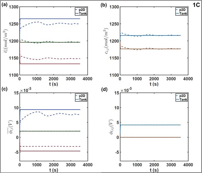
Figure 10. Comparison of liquid phase variables at 1C, namely (a) average concentrations  (b) interfacial electrolyte concentrations cij (c) average electrolyte phase potential
  and (d) interfacial potential ϕl, ij. The separator-positive electrode interface is the potential reference, hence ϕl, ij = 0. The negative-separator interface is indicated by the light blue and positive-separator interface by maroon. The average and interfacial values are plotted on identical scale to aid interpretation of the respective concentration and potential drops.
The concentration drop across the separator is ∼ 40 mol/m3 given its smaller thickness relative to the electrodes. Therefore, the diffusion coefficient at both interfaces is comparable in magnitude, since the concentration change is within 4%. Coupled with the comparable thicknesses of both electrodes (Table III), this results in similar magnitudes of interfacial concentration drops in both electrodes due to the imposition of flux continuity by the Tank Model as in Equation 41.
Figures 11a and 11b compares the concentrations at 5C discharge rate. The close agreement between the concentrations is notable, indicating the ability of the Tank Model equations to capture the concentration variations. The average concentrations in the electrodes agree within 5%, with near-exact agreement for the values in the separator, and at the interfaces. The transient dynamics and concentration drop in the electrodes for both models are qualitatively similar to the 1C case, though the magnitude of the concentration drop has increased to sustain the higher flux at 5C. The close agreement between the concentrations profiles suggests that the contribution of concentration overpotential errors to Vcell is not significant up to 5C for the cell parameters considered here. It also indicates the accuracy of the  approximation, likely due to the electrode thicknesses considered. It may be possible to refine these flux approximations by altering the diffusion lengths δi, ij. This can be used to in order to match the concentration profiles with attendant benefits for the accuracy of prediction of Vcell through the concentration overpotentials. For example, it is common in literature to assume a parabolic or cubic spatial dependence for ci in the electrodes.24,25,27,34,45 Applying volume-averaging on a parabolic profile in a given domain returns a value of
  , the use of which may result in more accurate predictions.32,34 It is worth noting however that the δi, ijvalue can be treated as an adjustable parameter that can be estimated, providing a representative measure of the diffusion length scales for a given operating situation. This allows more flexibility, in that different values may be adjusted for different domains without altering the model formulation, in contrast to assuming spatial profiles in a somewhat heuristic fashion, which entails rederiving the DAE system each time a spatial profile is changed.
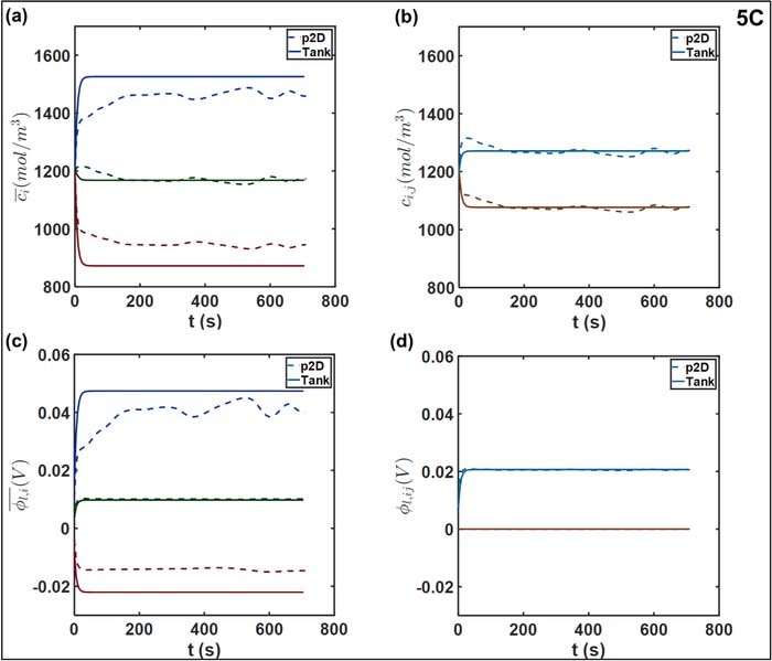
Figure 11. Comparison of liquid phase variables at 5C, namely (a) average concentrations  (b) interfacial electrolyte concentrations cij (c) average electrolyte phase potential
  and (d) interfacial potential ϕl, ij. The separator-positive electrode interface is the potential reference, hence ϕl, ij = 0. The values at the negative-separator interface are indicated by light blue curves and positive-separator interface by maroon curves. The average and interfacial values are plotted on identical scales to aid interpretation of the respective concentration and potential differences.
Electrolyte potential
Figures 10c and 10d depict the average and interfacial values of the electrolyte potential ϕl over a 1C discharge. Of note, the average values  rapidly reach a steady state for the Tank Model. We observe excellent agreement in the separator
  . This indicates the validity of the chosen flux approximations in the relatively thin separator, which also ensure agreement between the interfacial values ϕl, ij. This is a likely consequence of the charge conservation imposed by the Tank Model through Equation 56, which adjusts the values of interfacial potential to maintain the total liquid phase current iapp.
More significant differences are observed in the electrodes. In particular, the  value predicted by the p2D model exhibits substantial fluctuations, whereas the Tank Model predicts a steady state within ∼30 s of the discharge process. This qualitative difference is likely due to the errors in the prediction of average potential from the average pore-wall flux, owing to the non-uniform reaction distribution in the negative electrode, as discussed previously. The errors due to approximating the terminal overpotential based on the average
  in the Tank Model is thus manifested in
  , with the instantaneous deviation from the p2D model tracking the time-varying local reaction rates. In addition, substantial errors are observed at shorter timescales, where the Tank Model predicts the attainment of steady state. The maximum absolute value of this deviation is ∼3 mV, corresponding to approximately 40%. The choice of flux approximation is also likely to affect the deviation of the average value from that at the terminal, in addition to producing mismatches in ohmic drop.
In contrast, the uniform reaction distribution in the positive electrode results in a more spatially uniform overpotential profile over the discharge process, which is also reflected in the nature of the  profiles. The average values reach quasi-steady values differing by ∼1.5 mV. The sum of the average errors in both electrodes value is ∼3 mV, which is comparable in magnitude to the voltage errors in Figures 5a and 5d. The main contributions to the error Vcell are thus the liquid-phase potentials in the electrodes.
These effects are further accentuated at 5C, as illustrated in Figures 11c 11d. In particular, the initial deviation in  has increased beyond 10 mV, with a commensurate increase in average errors in both electrodes. The deviations in both electrodes are ∼ 7 mV, indicating comparable errors in ohmic drops. Interestingly, the profile for
  from the p2D model also shows a slight fluctuation at t ∼ 300 s, corresponding to the non-uniformities in j1 at 5C as seen in Figure 9a. The total average error in electrolyte potentials is comparable to the values of Figures 5c and 5d. This indicates a contribution of errors in
  to Vcell through
  . The separator
  and interfacial values ϕl, ij are in close agreement even at 5C, except for relatively small errors in ϕl, 23 during the approach to steady state.
Refinement of the gradient approximation for  may help reduce errors by matching the ohmic drops across the electrodes, and by improving predictions of reaction overpotential. As with electrolyte concentration, it is common to assume polynomial profiles for the spatial variation of ϕl.26,32 Similar adjustments of the analogous length-scale approximations may help improve estimates of the migration contribution to ionic current, helping reduce errors in the estimation of both ohmic drops and reaction overpotentials. Preliminary studies suggest that altering gradient approximations marginally increases the errors for
  and
and  , and thus for the positive overpotential
  , but this error is more than balanced by the reduction in errors for
  ,
,  and the overall electrolyte ohmic drop.
Interfacial fluxes
Figure 12a depicts the comparison of the Tank Model approximations Ni, j with the actual interfacial values from the p2D model. The interfacial fluxes exhibit excellent agreement even with the somewhat simple approximations for the Tank Model. Discrepancies in the temporal profiles are observed at relatively short timescales, where the full model predicts a different trajectory for the approach to steady state and subsequent minor fluctuations (not shown). However, this error is less than 1% even for 5C discharge, as in Figure 13a. The close match between fluxes is observed once the steady state gradients have been established at approximately 30 s, which, expectedly, is of the order of the diffusion timescale for the electrolyte. For the Tank Model, the match between the fluxes at the two interfaces is also consistent with the observation of nearly equal interfacial concentration drops and comparable electrode thicknesses, as discussed in the section on electrolyte concentration. There is a rapid establishment of steady state. We expect the approximations to reduce in validity as the current density is increased further. Errors will also arise if the characteristic timescales for different processes are increased, which will result in significant spatial gradients (analogous to the reaction distribution). This in turn is expected to result in errors of concentration overpotentials, with its manifestation in errors in Vcell.
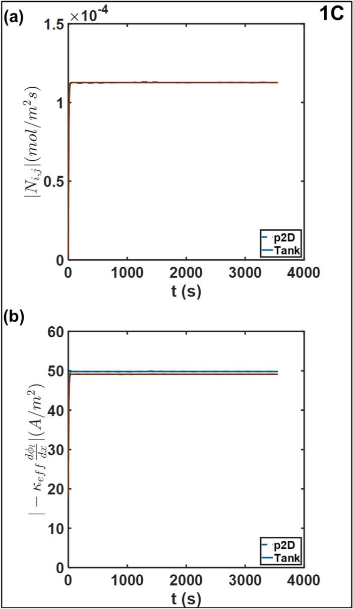
Figure 12. Comparison of (a) interfacial molar flux Ni, j and the (b) ohmic contribution to liquid phase current density at the positive-separator interface (maroon) and negative-separator negative (blue), at 1C. The operating current density iapp is ∼17.5 A/m2.
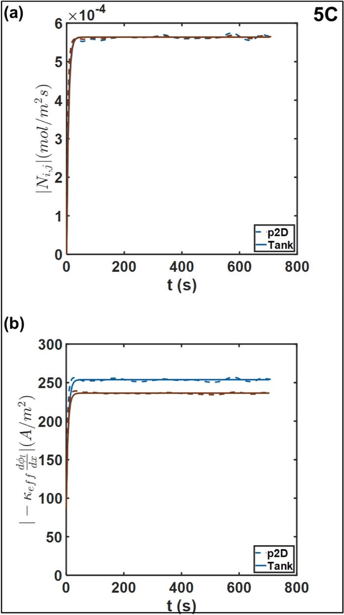
Figure 13. Comparison of (a) interfacial molar flux and the (b) ohmic contribution to liquid phase current density at the positive-separator interface (maroon) and negative-separator negative (blue), at 5C. For reference, the operating current density is ∼87 A/m2.
Figure 12b compares the approximations for the ohmic contribution to the electrolyte current density at 1C, to evaluate the approximations for the electrolyte potential gradients. Here too we observe substantial agreement with respect to the p2D model. This is expected given the match in the interfacial mass flux predictions above. The Tank Model ensures charge conservation at the interface through Equations 52. Agreement between the diffusional contributions forces the equality of the ohmic contributions to maintain the current density at the interfaces. The relative error is comparable even at 5C, as depicted in Figure 13b. There is a slight discrepancy in values during the approach to the quasi-steady value and in subsequent fluctuations, which tracks the errors in electrolyte potentials discussed previously.
Given the close agreements in predicted concentrations and concentration overpotentials, the flux approximations for may be modified to reduce errors in  and
and  . One easy way to achieve this could be to use a length scale approximation corresponding to a higher order polynomial profile. For the cell and current densities considered in this article both concentration overpotentials and liquid phase ohmic drops are small relative to the 'thermal voltage' RT/F.5,18 However, the errors in ohmic potential drop and concentrations could cause errors in Vcell at higher current densities, which will be reflected in systematic errors in both |Ni, j|and
  .
.
Case study: thick electrodes
The tanks-in-series model thus needs to be examined in light of different limiting performance scenarios, especially for situations in which significant spatial gradients can arise across the electrodes, giving rise to polarizations that are underestimated – e.g. extremely high rates of discharge, or very thick electrodes. This is related to the key assumptions in the Tank Model, namely the interfacial fluxes, which determines the accuracy of the corrections for liquid phase effects.
The impacts of these approximations are now studied in a special case, by the comparison of the Tank Model for the case of a cell with relatively thick electrodes, which may be of salience for high-energy density batteries.51,52 For this case study, the electrode thicknesses l1 and l3 were increased by a factor of 6 while holding all other parameters constant. Thus, the individual capacities of each electrode increase by a factor of 6, while their ratio is held constant. For a consistent comparison with the Base Case, the model was compared at a 5C/6 C-rate, corresponding to the current density iapp equivalent to the 5C discharge for the Base Case. The modified parameter values are listed in Table V.
Table V. Modified Parameters for the 'thick electrode' case.
| Parameter | Base Case Value | Modified Value |
|---|---|---|
| Positive Electrode Thickness (μm) | 36.55 | 219.3 |
| Negative Electrode Thickness (μm) | 40 | 240 |
| 1C Discharge Current Density (A/m2) | −17.54 | −105.24 |
| C-rate | 5 | 5/6 |
| Se | 0.1 | 0.53 |
For this '6x case', significant electrolyte diffusion limitations and ohmic drops are expected to arise compared to the Base Case. A modified parameter Se based on Doyle et al. can be used as a measure of expected diffusion limitation.5,53
Thus
![Equation ([60])](https://content.cld.iop.org/journals/1945-7111/167/1/013534/revision1/d0060.gif)
This factor is thus the ratio of the characteristic time for electrolyte diffusion to the total discharge time, higher values suggesting exacerbated diffusion resistances.
The voltage-time discharge curve for this case is depicted in Figure 14. Here we can observe the large liquid phase polarization and spatial non-uniformities that SPM is clearly unable to capture, and instead predicts near-complete cell utilization. The p2D model predicts termination of discharge at an intermediate time point, likely owing to severe electrolyte depletion in the positive electrode. What is noteworthy however is the prediction of the Tank Model, which predicts a premature termination but within 5 minutes of the discharge process. This is despite substantially improved agreement compared to SPM over the small portion of its operation. This suggests substantial error in the prediction of ci and ϕl, i. This can now be seen in Figure 15, which compares the average concentration predictions from the two models. In particular, the Tank Model predicts the  being driven to zero at t ∼5 minutes, which coincides with the termination of discharge. The
  values disagree by more than 20%, while the Tank Model predicts
  at t ∼ 300 s, in contrast to the actual value of ∼500 mol/m3. This discrepancy thus suggests the limitation of the diffusive flux approximations, which substantially overestimate the concentration gradients. One possible reason for this error is that the diffusion layers have not built up to their steady state value, as also indicated by the diffusivity parameter Se. The errors due to the resulting flux approximations may be circumvented by refining the same, or by the use of a time-dependent exponential correction for the length approximation as suggested by some workers.32,54 The time constants for this exponential change may be defined based on characteristic diffusion timescales.
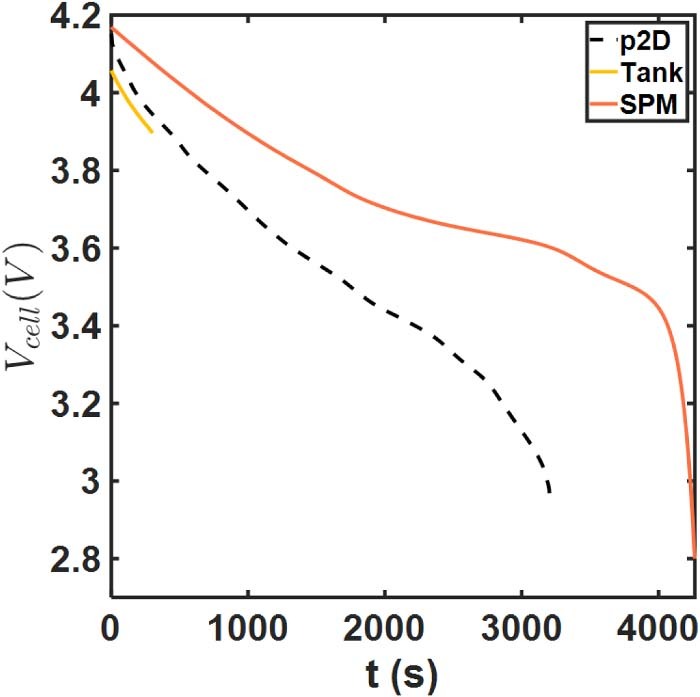
Figure 14. Discharge curve comparisons for the thick electrode case.
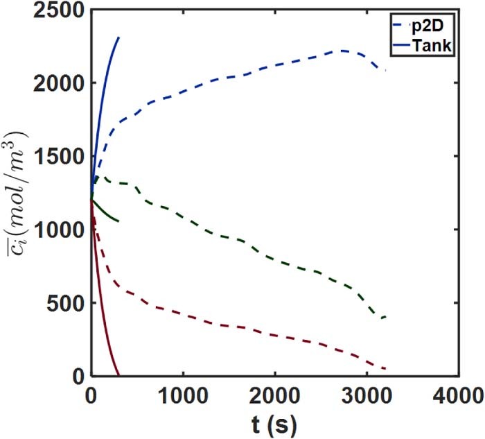
Figure 15. Average concentration  comparison for the thick electrode case. The approximate Tank Model predicts zero electrolyte concentration in the positive electrode at a relatively short time (t∼300 s).
This example thus demonstrates a combination of design and operating parameters in which the Tank Model has reduced performance and necessitates improved approximations. In particular, the large polarizations considered in this example may be encountered for the Base Case cell as well, such as during high-current dynamic and pulsed operation. A more comprehensive analysis is useful to establish the parameter combinations at the cell level that deem the Tank Model useful. The limits of a BMS that uses such a model can also be defined through such an analysis.
Comparisons against other reduced-order models
In this article, the Tank Model is compared against SPM because of its substantial ubiquity in advanced BMS applications, as it continues to be the model of choice when physical detail is desired. In introducing the Tank Model, we seek to propose an alternative for various applications where SPM is substantially common. However, for additional perspective, this section discusses the error metrics of the Tank Model relative to a recent version of the SPMe, which corrects SPM with electrolyte dynamics as mentioned previously.18 For this study, the electrode parameters from Ref. 18 were chosen, in addition to electrolyte transport correlations from Ref. 42. The representative values of electrolyte transport properties required by the SPMe formulation were evaluated at the initial electrolyte concentration.
The error metrics up to 3C discharge rate are illustrated in Figure 16. The substantial improvement in error in going from SPM to lumped electrolyte models is evident, particularly at 3C, where the RMSE reduction is nearly three-fold for SPMe. However, the Tank Model exhibits even lower error (13 mV vs. 35 mV). This suggests more accurate estimation of concentration overpotentials and liquid phase ohmic drops for the chosen parameters. The SPMe uses representative values, whereas the Tank Model only requires the evaluation of electrolyte transport properties at the interfaces. Consequently, the concentration-dependent transport properties can be included in an efficient manner. The expressions in SPMe may need to be rederived to account for these variations.
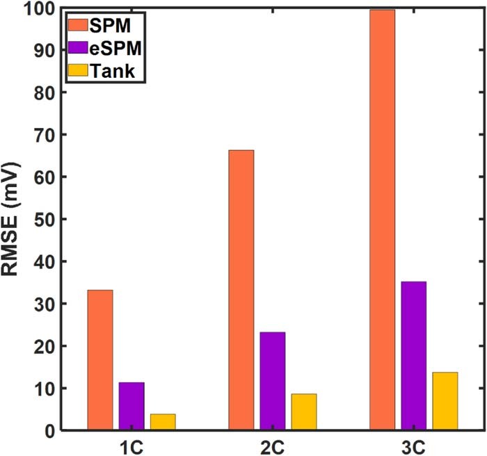
Figure 16. Representative comparisons of SPM (peach), SPMe (purple), and the Tank Model (gold). The p2D model is used as the benchmark.
Computational performance
Computational times for the Tank Model are listed in Table VI. For the Tank Model, each conservation law in the electrolyte phase is replaced by its volume-averaged form, while the solid phase in each electrode is replaced by 3 linear DAEs. The original ∼ 200 – 1000 DAEs are thus replaced by 14 average conservation equations. This results in a 1C discharge curve being simulated in ∼ 2 ms, in contrast to >1000 ms for a standard Finite Difference implementation. The computational speed of this model is comparable to fast SPM implementations. The Tank Model is also competitive with the state-of-the-art reformulated p2D model from our group, achieving up to an order of magnitude reduction in computation time. The mathematical similarity of the Tank Model to the reformulated model with n = (1,1,1) collocation prompts the question as to why the (1,1,1) reformulated model is not used instead of developing the Tank Model. This is because the proposed model is conservative and exhibited higher accuracy. In addition, it can be rewritten so as to contain fewer adjustable parameters compared to reformulated models. Increasing the accuracy and numerical convergence of reformulated models requires using its ability to guarantee convergence for different chemistries, parameters and operating conditions by increasing the number of collocation points.
Table VI. Representative computational performance metrics for the Tank Model.
| Number of | Computation | |
|---|---|---|
| Model and Implementation | DAEs | time (ms)* |
| p2D – Finite Difference (50,35,50) | 986 | 1493 |
| p2D - Reformulated | 30–150 | 5–20 |
| Tank Model | 15** | 2.1 |
*Average of N = 3 simulation runs for a 1C discharge. It must be noted that the simulation time and memory consumption is a strong function of the computing environment as well as error tolerances for both initialization and simulation. **Including the equation for cell voltage.
Recasting the tank model
Recalling the volume-averaged electrolyte Equations 46–48 of the Tank Model, we have
![Equation ([61])](https://content.cld.iop.org/journals/1945-7111/167/1/013534/revision1/d0061.gif)
![Equation ([62])](https://content.cld.iop.org/journals/1945-7111/167/1/013534/revision1/d0062.gif)
![Equation ([63])](https://content.cld.iop.org/journals/1945-7111/167/1/013534/revision1/d0063.gif)
The above equations may be conveniently written as
![Equation ([64])](https://content.cld.iop.org/journals/1945-7111/167/1/013534/revision1/d0064.gif)
![Equation ([65])](https://content.cld.iop.org/journals/1945-7111/167/1/013534/revision1/d0065.gif)
![Equation ([66])](https://content.cld.iop.org/journals/1945-7111/167/1/013534/revision1/d0066.gif)
Where the governing equations have been expressed in terms of equivalent 'mass transfer' coefficients, volume and source terms. In the above equations, the  have units of mass transfer coefficient (m/s), and Vl, i denotes the electrolyte volume (per unit area) in region i with units of length. The transport parameters in the electrolyte current balance 56 may also be grouped similarly
![Equation ([67])](https://content.cld.iop.org/journals/1945-7111/167/1/013534/revision1/d0067.gif)
Where, the thermodynamic factor v(cij) = 1 for simplicity. Here,  have units of S/m2. The lengths used in the flux approximation, which for this case is
  , are present in the expressions for Kij and Sij. Estimating these quantities is equivalent to deriving a suitable flux or gradient approximation. For constant diffusivity, the electrolyte concentration equations constitute a coupled linear system of Ordinary Differential Equations with constant coefficients. The form of these equations suggests a possible parameter estimation strategy in which the Tank Model is matched against experimental data by direct estimation of the 'consolidated' transfer coefficients. Variations due to concentration-dependent transport properties, or transients in which the 'steady state layer' is attained over a characteristic timescale comparable to discharge time can potentially be handled by estimating average values over the course of the process. The similarity of the mathematical model to conventional Continuous Stirred Tank Reactor (CSTR) systems is noteworthy and suggests scope for exploiting the extensive control theory developed for CSTR systems.
Conclusions and Future Work
An efficient, conservative model for lithium-ion batteries is presented, which uses a Tanks-in-Series approach to generate approximate equations for electrolyte dynamics. Despite the loss of information due to volume-averaging, the additional equations result in a nearly four-fold reduction in error compared to typical SPM at high (5C) discharge rates. While the Tank Model achieves excellent accuracy with respect to the full p2D model for the cell considered in this article (<0.4% error), even better performance is expected for electrodes with inherently more uniform reaction distributions. The model formulation provides for the convenient refinement of flux approximations and estimation to increase accuracy for more aggressive parameter combinations. The model retains the computational simplicity of SPM-like models, with the millisecond computation time making it a candidate for a replacement of SPM in the simulation of large series-parallel configurations of cells. The model may also be used for long cycle simulation and parameter estimation toward modeling capacity degradation, and the evaluation of models for the same.
The generalized methodology developed herein can be applied to electrochemical models for more complex systems, including conversion chemistries such as Li-sulfur and lead-acid batteries. The application of this technique for a PDE model for Li-sulfur batteries will be communicated in a future article. Thermal effects, and the resulting interplay with transport and kinetic processes will introduce an additional dimension of complexity. Application of this methodology to the energy balance equations is a key next step and a logical extension of the current work. Future work also includes developing approximate analytical and perturbation solutions for this model. We envisage the ultimate use of this model in state and parameter estimation, real-time control and advanced BMS.
In this article, we defined the scope of our work as the detailed development of the Tanks-in-Series model, and evaluation of its predictions against the full p2D model in terms of accuracy and computational speed. Some comparisons against SPM were provided to illustrate the improvement over the most common electrochemical models for advanced BMS. While conceptual differences between this model and other methodologies in literature were touched upon, a detailed comparison was avoided to maintain focus on the details of the generalized Tanks-in-Series methodology. The literature on reduced-order p2D models is vast with each technique possessing its advantages, limitations, and conditions for applicability. Future work will involve more detailed analyses of the differences in the Tanks-in-Series approach and other methods, and their impact on key performance measures and model predictions.
Acknowledgments
The authors would like to thank the U.S. Department of Energy (DOE) for providing partial financial support for this work through the Advanced Research Projects Agency (ARPA-E) award number DE-AR0000275, and the Advanced Battery Material Research (BMR) Program (Battery 500 Consortium). The authors would also like to thank the Clean Energy Institute (CEI) at the University of Washington, the Washington Research Foundation (WRF) and Texas Materials Institute for partial monetary support of this work.
ORCID
Venkat R. Subramanian 0000-0002-2092-9744