
Abstract
Lithium-ion (Li-ion) batteries find wide application across various domains, ranging from portable electronics to electric vehicles (EVs). Reliable online estimation of the battery's state of health (SOH) is crucial to ensure safe and economical operation of battery-powered devices. Here, we developed three deep learning models to investigate their potential for online SOH estimation using partial and random charging data segments (voltage and charging capacity). The models employed were developed from the feed-forward neural network (FNN), the convolutional neural network (CNN) and the long short-term memory (LSTM) neural network, respectively. We show that the proposed deep learning frameworks can provide flexible and reliable online SOH estimation. Particularly, the LSTM-based estimation model exhibits superior performance across the test set in both direct learning and transfer learning scenarios, while the CNN and FNN-based models show slightly diminished performance, especially in the complex transfer learning scenario. The LSTM-based model achieves a maximum estimation error of 1.53% and 2.19% in the direct learning and transfer learning scenarios, respectively, with an average error as low as 0.28% and 0.30%. Our work highlights the potential for conducting online SOH estimation throughout the entire life cycle of Li-ion batteries based on partial and random charging data segments.
Export citation and abstract BibTeX RIS

This is an open access article distributed under the terms of the Creative Commons Attribution 4.0 License (CC BY, http://creativecommons.org/licenses/by/4.0/), which permits unrestricted reuse of the work in any medium, provided the original work is properly cited.
Li-ion batteries have been widely used in EVs due to their compact size, lightweight, high energy and power density, low self-discharge rate and long lifespan. 1–5 However, ensuring the safe and reliable operation of batteries has posed high requirements and significant challenges for battery management technologies, including critical tasks such as battery state estimation, fault diagnosis, and thermal management. 6,7 SOH estimation, one of the important functions in a battery management system (BMS), 8 plays a key role in evaluating the aging state and remaining useful life of batteries, as well as in predicting the driving mileage for EVs. 9 Up until now, researchers have proposed several approaches for battery SOH estimation, which can be classified into three categories: direct measurement, model-based methods, and data-driven methods. 10 Direct measurement requires a complete charging or discharging process to directly determine the battery's SOH. Although this approach is much straightforward, it can be limited for practical implementation in EVs. 11
Model-based methods can be further categorized into empirical/semi-empirical model-based methods, equivalent circuit model-based methods, and electrochemical model-based methods. 12 Specifically, an empirical/semi-empirical model 13–15 describes the battery behavior by various functions and formulas and fit the battery degradation with time, cycles, or other factors. Miao et al. 14 developed a battery degradation model using the unscented particle filter algorithm to predict the battery's remaining useful life, achieving a prediction error of less than 5%. Tseng et al. 15 employed regression models with particle swarm optimization to monitor battery degradation, finding that using fully discharged voltage and internal resistance as aging parameters yielded better estimation results than cycle number. The empirical/semi-empirical models can exhibit a high level of computational efficiency, while they are usually developed based on a specific set of working conditions, thus resulting in poor applicability for other conditions. 16 The equivalent circuit models and electrochemical models are generally developed on the theoretical and fundamental understanding of electrochemical behaviors inside a battery. 17 An equivalent circuit model 18–20 describes battery characteristics through a specific circuit network comprised of electrical components such as resistors and capacitors. Galeotti et al. 18 utilized electrochemical impedance spectroscopy (EIS) to characterize lithium polymer batteries and achieved SOH evaluation with a maximum error of 3% for standard cells and 8.66% for anomalous cells. Lyu et al. 20 proposed a time-domain impedance spectroscopy technique combined with an equivalent circuit model and the genetic algorithm, achieving SOH estimation accuracy within 10% of 240 cycles for Li-ion batteries in aging experiments. The equivalent circuit models are established based on battery behavior assumptions and simplified mathematical calculations, thus leading to limited accuracy and robustness. 21 In contrast, an electrochemical model 22–24 can properly reflect the electrochemical reaction processes occurring inside a battery cell to a great extent. Xiong et al. 22 proposed an electrochemical model-based SOH estimation method based on the pseudo-two-dimensional (P2D) model. The finite analysis and numerical computation methods were used to solve the mathematical equations. They achieved a SOH estimation error bounded to 3%. Hosseininasab et al. 23 derived a fractional battery model from partial differential equations (PDEs) governing the P2D model and realized adaptive estimation of battery resistance and capacity. In dynamic load conditions, the capacity estimation error decreased from 8% to 0.1% after eight iterations. However, the electrochemical models usually require detailed information about the battery cell, such as the porosity of the electrode and the conductivity of the electrolyte. 3 Furthermore, these models are generally developed from sophisticated PDEs, thus requiring large memory and high computational power for transient PDE solving. 12
Recently, data-driven methods have gained much attention due to several advantages. For instance, these methods have the potential to analyze a wide range of aging mechanisms and working conditions without requiring prior knowledge of electrochemical behaviors occurring inside battery cells. 25 The data-driven methods can be classified into two categories: traditional machine learning methods and deep learning methods. 17 The traditional machine learning methods 24–27 generally use features manually extracted from battery data as the estimation model input. Yang et al. 27 proposed a novel Gaussian process regression model based on charging curves, extracting four specific parameters to accurately reflect battery aging phenomena from different perspectives. Hu et al. 28 developed a non-linear kernel regression model based on k-nearest neighbor regression and five charge-related features were used to estimate battery's SOH, achieving root mean square errors below 2.00% and maximum errors below 5%. These methods demonstrate fast convergence and considerable accuracy, while requiring domain knowledge to obtain proper features from a big test dataset. 29 On the contrary, the deep learning methods 17,29–32 can directly employ measured variables such as voltage, current, and temperature as the model input without manual feature extraction. Shen et al. 31 developed a deep CNN model for battery discharge capacity estimation using voltage, current, and charge capacity data, demonstrating higher accuracy and better robustness than traditional machine learning models. Choi et al. 32 compared the performance of three models based on FNN, CNN, and LSTM for battery capacity estimation. They found that when using multi-signal input (voltage, current, temperature), the mean absolute percentage error of the model decreased by 25% to 58% compared to single-signal input. Kaur et al. 17 investigated the effects of model complexity and signal type on the performance of three neural network models, with the LSTM neural network model demonstrating the best performance, and battery temperature carrying less significance for capacity estimation. Hence, compared with the traditional machine learning methods, the deep learning methods can be easier to realize automatic feature extraction and model training. This can save effort for feature derivation and ease online estimation for enabling practical application in EVs.
While researchers have conducted numerous studies on battery SOH estimation techniques using various machine learning and deep learning models in the past few years, most of these studies were conducted under simple working conditions, such as constant-current (CC) or constant-voltage (CV) charging and discharging with different C-rates. 17,25–34 These conditions can significantly differ from practical operating conditions which involve complex and transient discharging behaviors influenced by factors such as road conditions, traffic trends, and driving behaviors. Additionally, the input data for the estimation models in these studies was generally derived from the charging or relaxation process. For the charging process, the input data was usually derived from specific voltage/state of charge (SOC) ranges, 25,27,29,31,33 or extracted from entire charging processes. 17,26,28,30,32 For the relaxation process, the battery cell was always required to be fully charged to 100% SOC. 34 Unfortunately, in both cases, estimation models are not flexible enough for practical application in EVs.
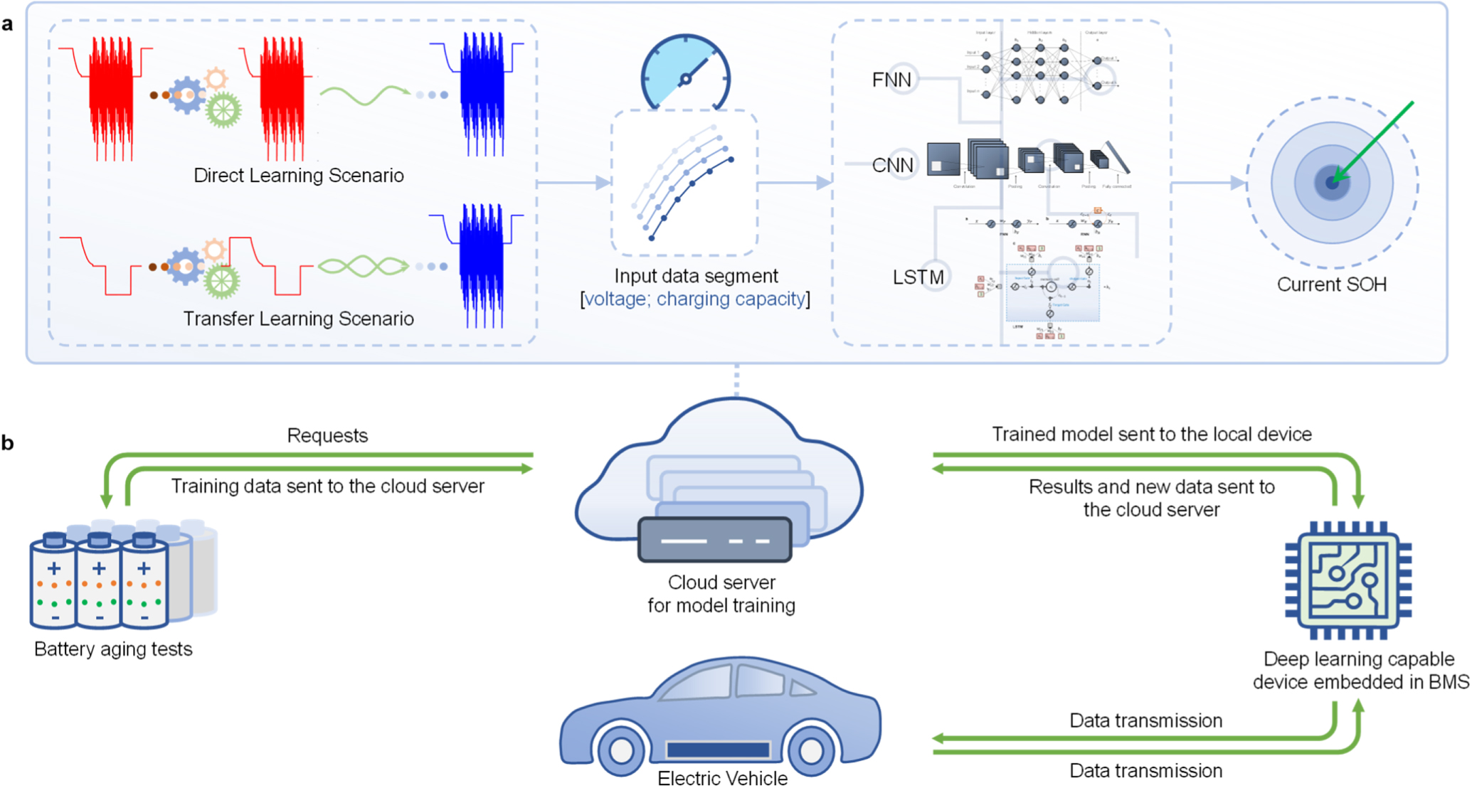
To overcome these limitations and further explore the scalability of deep learning models, we developed three mainstream deep learning models based on FNN, CNN and LSTM frameworks, respectively, to explore their potential for online SOH estimation of Li-ion batteries based on partial and random charging data segments. Furthermore, we conducted a comparative study among the three models, evaluating the accuracy of online battery SOH estimation in both direct learning (complex training set to estimate complex operating conditions) and transfer learning (simple training set to estimate complex operating conditions) scenarios. The overview of the present framework is shown in Fig. 1. First, the cloud server stores and processes the battery data gathering from experimental aging tests to train deep learning models. Second, the trained model is sent to the local device embedded in the EV and used for online SOH estimation. Finally, the random battery data generated during the vehicle operating process can be used for current SOH estimation as well as for model improvement. Our work aims to provide valuable insight into the accurate and flexible online SOH estimation for Li-ion batteries throughout the battery life cycle during complex operating conditions, without disturbing the ongoing charging or discharging process.

Figure 1. An overview of the present framework: (a) the procedure of battery SOH estimation; (b) the flow chart of potential application of deep learning models in EVs.
Download figure:
Standard image High-resolution imageMethodology
Battery aging test
The battery aging test was performed by the NEWARE testing system on a commercial 18650 li-ion battery cell. Figure 2 shows the schematic of the testing system, and the key parameters of the battery are listed in Table I.

Figure 2. Schematic of the battery testing system.
Download figure:
Standard image High-resolution imageTable I. Key parameters of the present 18650 li-ion battery.
| Parameter | Value |
|---|---|
| Chemical component of cathode | LiNiCoAlO2 (NCA) |
| Chemical component of anode | Graphite |
| Nominal capacity | 3000 mAh |
| Range of working voltage | 2.5–4.2 V |
| Nominal voltage | 3.6 V |
| Charging current at 1 C | 3 A |
In this work, eight 18650 cells were employed for the test, and they were sorted evenly into two groups, namely 1C-constant and 3C-WLTC cycles. Each basic cycle consists of four steps: charge, rest, discharge, and rest. The cells were charged using the CC-CV protocol. Firstly, a cell is charged at a constant current of 3 A until the voltage reaches an upper limit of 4.2 V. After that, the cell is supplied with a constant voltage of 4.2 V charging until the current drops to 0.15 A. Following this, the cell undergoes a rest step of 30 min. Finally, the cell is discharged until the battery voltage drops to 2.5 V, which is then followed by a rest period of 30 min. The discharging protocols are different for the two test groups, thus resulting in different aging paths. The 1C-constant cells are discharged at a constant current of 3 A, while the 3C-WLTC cells are set to work at the Worldwide harmonized Light vehicles Test Cycle (WLTC) 35 protocol with a maximum value of 9 A, which mimics complex urban and rural driving conditions including low, medium, high and extra high-speed driving modes. Figures 3a and 3b show the current-time curves for the 1C-constant and 3C-WLTC cycling processes, respectively. To minimize the influence of the ambient temperature, the test room was maintained at a constant temperature of 25 °C by a large ventilation system.

Figure 3. Current-Time curves for the battery aging tests corresponding to: (a) the 1C-constant cycling process; (b) the 3C-WLTC cycling process.
Download figure:
Standard image High-resolution imageBasic signals such as voltage ( ) and current (
 ) can be directly measured by the test system. Battery capacity (
 ) can be obtained by adding the capacity increment (
 ) to the initial capacity (
 ) as shown in Eq. 1. Here,
  is the integral of current (
 ) with respect to time (
 ) as shown in Eq. 2:


Deep learning models
Feed-forward neural network (FNN)
FNN is the earliest and simplest neural network model, which includes an input layer, an output layer and several hidden layers (Fig. 4). 36 The neurons in each hidden layer are fully connected with the neurons in adjacent layers, but no loop is formed. In FNN, information has only one flow direction, that is, forward. The structure of the input data determines the size of the input layer, and the parameters in the hidden layer neurons are all learnable and determined through iterative training. The size of the output layer depends on the problem under study.

Figure 4. Schematic of the FNN structure.
Download figure:
Standard image High-resolution imageConvolutional neural network (CNN)
CNN is a regularized version of FNN. Unlike the fully connected structure of FNN, the convolution operation in CNN realizes local connection and weight sharing between neurons in adjacent layers. 37 Hence, a CNN model has relatively fewer parameters. Generally, a CNN is composed of convolutional layers, pooling layers and fully connected layers 38 (Fig. 5). The convolutional and pooling layers are used for feature extraction and feature map compression, respectively. Global features of input data can be obtained by performing multi-step convolution and pooling operations. This scheme enables an efficient extraction of main features and a significant reduction in computational complexity. Finally, regression or classification can be achieved through the fully connected layers.

Figure 5. Schematic of the CNN structure.
Download figure:
Standard image High-resolution imageLong short-term memory neural network (LSTM)
LSTM was developed from recurrent neural network (RNN). Compared with FNN (Fig. 6a), RNN contains an additional memory cell as shown in Fig. 6b. The output of FNN is completely determined by the current input, as formulated in Eq. 3:

where  and
and  represent the input and output of a neuron, respectively,
  represents the present time step,
  is the weight parameter, and
  is the bias parameter. However, for RNN, the memory cell makes its output not only depend on the input of the current time step, but also on the output of the last time step, as shown in Eqs. 4–6:


where  represents the output,
  and
and  represent the previous and next time steps, respectively,
 and
and  represent the weight, bias, and memory parameters, respectively. This makes RNN more suitable for processing time-series data. However, the gradient vanishing problem may occur when using traditional RNN and dealing with long-time sequences.
39
To solve this problem, LSTM was proposed as an evolutionary RNN with the simple memory cell further evolving into a memory module. This module contains three basic gates (input, output and forget gates), which control the proportion of information stored in the memory cell and output (Fig. 6c).
40
represent the weight, bias, and memory parameters, respectively. This makes RNN more suitable for processing time-series data. However, the gradient vanishing problem may occur when using traditional RNN and dealing with long-time sequences.
39
To solve this problem, LSTM was proposed as an evolutionary RNN with the simple memory cell further evolving into a memory module. This module contains three basic gates (input, output and forget gates), which control the proportion of information stored in the memory cell and output (Fig. 6c).
40

Figure 6. Schematics of the basic structures of (a) FNN, (b) RNN and (c) LSTM.
Download figure:
Standard image High-resolution imageThe forward propagation process of a unit in the LSTM neural network is shown in Eqs. 7–12:


where  is the input of a LSTM unit,
  is the generated new memory,
  and
and  are the hidden outputs of the unit at the present time step and last time step,
 and
and  represent the input gate, forget gate, and output gate, respectively,
  is the previous state of the memory cell,
  is the present state of the cell,


 and
and  are the weight parameters,

 and
and  are the bias parameters, and

 represent activation functions.
Implementation details
Each learning model is implemented by Tensorflow in Jupyter Notebook on a workstation, which is equipped with an Intel Xeon(R) Gold 5218 R CPU (2.10 GHz), an NVIDIA GeForce RTX 3090 GPU, and 512 GB of memory. The structures and hyper-parameters of models are designed by the validation set. The mean squared error (MSE) is used as the loss function to compute the distance between the predicted output and target output of the training data. The Adam optimizer is used to update the network weights iteratively based on a training set with a learning rate of 0.001. The number of training epochs is set to 500 and a batch size of 400 is used. The Rectified Linear Unit (ReLU) 41 is used as the activation function. The detailed information of the model structures is listed in Table II.
Table II. Structures of the deep learning models. In the CNN, a*b@c means c filters with a size of a*b, and the stride is set to (d, d).
| Model | Structure | Number of parameters |
|---|---|---|
| FNN |
| 2801 |
| CNN |
| |
| 3117 | |
| ||
| LSTM |
| 23131 |


Data preprocessing
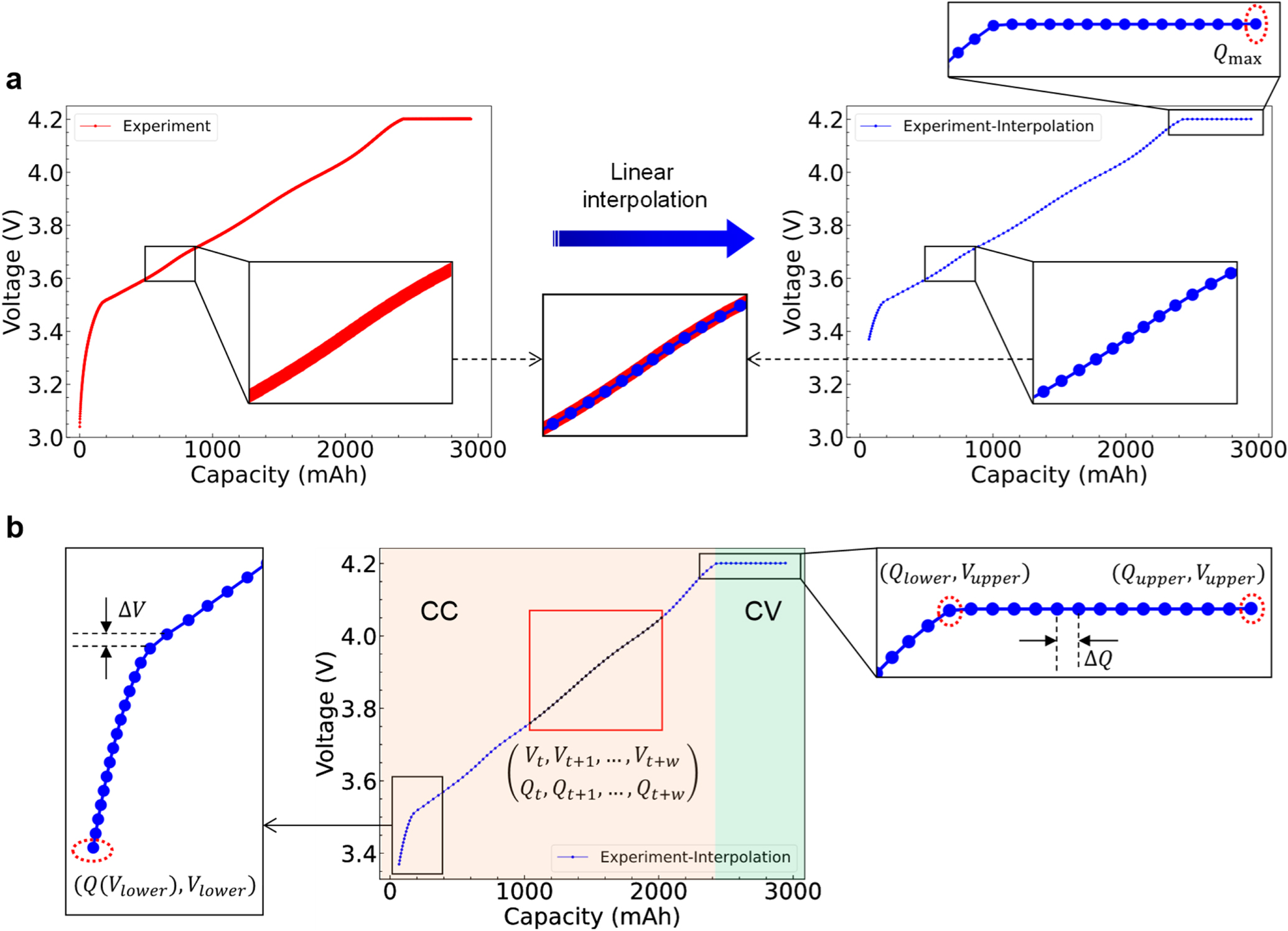
The battery cycle dataset is collected during the aging test (Figs. 2 and 3). Since the traffic conditions and the driving behavior can differ for each EV, the discharging behavior of an EV can be very complex during real driving scenarios. However, battery charging process in EVs typically follows a standardized protocol, namely CC-CV protocol (Fig. 3), which is more stable and controllable. Hence, the charging dataset is selected as the training set and utilized for online SOH estimation. Figure 7 shows the detailed data processing procedure used for the model training and testing. To obtain the model input, linear interpolation is performed on the original experimental V–Q charging curve to obtain the interpolated curve (Fig. 7a). This enables a constant voltage interval (0.01V) between every two adjacent points in each sequential CC charging data segment. The maximum capacity can be read directly from the V–Q charging curve, which quantitively reflects the current battery aging state (Fig. 7a). In this context, the V-Q charging curve can be divided into two parts: the CC part and CV part (Fig. 7b), respectively, as expressed by Eq. 13:

where  corresponds to the CC charging process,
  denotes the lower voltage limit,
  (
( ) represents the upper voltage limit, and
  is the sampling interval of the voltage. Here,
  corresponds to the CV process,
  denotes the lower capacity limit,
  (
( ) represents the upper capacity limit, and
  is the sampling interval of the capacity. Finally, the V-Q curve can be encoded into a
  matrix
![$\left.{Q}_{1},{Q}_{2},\,\ldots ,\,{Q}_{N+1},{Q}_{N+2},\,\ldots ,\,{Q}_{M+N+2}\right].$](https://content.cld.iop.org/journals/1945-7111/170/9/090537/revision2/jesacf8ffieqn69.gif) Each element in the matrix represents the first value of the corresponding sequential data segment (Fig. 7b).
Each element in the matrix represents the first value of the corresponding sequential data segment (Fig. 7b).

Figure 7. Schematic of the data processing steps: (a) original experimental data and the result of linear interpolation,  is the estimation model output; (b) a sample of charging segment on the V-Q charging curve.
Download figure:
Standard image High-resolution imageThe battery charging process in practical EV scenarios is often incomplete, resulting in incomplete charging data segments collected in real time. Specifically, an available segment can be represented as ![${X}_{0i}=\left[{V}_{t},{V}_{t+1},\,\ldots ,\,{V}_{t+w};{Q}_{t},{Q}_{t+1},\,\ldots ,\,{Q}_{t+w}\right],$](https://content.cld.iop.org/journals/1945-7111/170/9/090537/revision2/jesacf8ffieqn71.gif)
 Figure 7b shows the schematic of a data segment which includes both the voltage and capacity sequences. In this work, each segment comprises 30 points of a V-Q charging curve, resulting in 69 segments within a charging cycle. Considering the data loss risk of EVs as well as the convenience and flexibility for data processing, the capacity sequence was converted to
 ![$\left[\left({Q}_{t}-{Q}_{t}\right),\left({Q}_{t+1}-{Q}_{t}\right),\ldots ,\left({Q}_{t+w}-{Q}_{t}\right)\right],$](https://content.cld.iop.org/journals/1945-7111/170/9/090537/revision2/jesacf8ffieqn73.gif) and the segment becomes
and the segment becomes ![${X}_{i}=\left[{V}_{t},{V}_{t+1},\,\ldots ,\,{V}_{t+w};0,{\rm{\Delta }}{Q}_{t+1},\,\ldots ,\,{\rm{\Delta }}{Q}_{t+w}\right].$](https://content.cld.iop.org/journals/1945-7111/170/9/090537/revision2/jesacf8ffieqn74.gif) This means the input segment can be obtained directly from an arbitrary EV charging period, which is independent of the historical data in BMS.
This means the input segment can be obtained directly from an arbitrary EV charging period, which is independent of the historical data in BMS.
To improve the model accuracy and speed up training convergence, the input data is usually normalized before being fed into the neural network. In this work, the min-max normalization was adopted to rescale the segments into the range of [0, 1] without disturbing the data distribution, as shown in Eq. 14:

where  is the normalized input,
  is the number of samples in the training or test set,
  is the collection of
  in the training set for all charging cycles,
  and
and  represent the minimum and maximum values of the training data, respectively.
Considering the difference between lab test conditions and EV driving conditions, we employed two basic scenarios to evaluate the performance of the deep learning models, i.e., the direct learning scenario and the transfer learning scenario. For direct learning, the model is trained and tested under complex conditions. For transfer learning, the model is trained under simple conditions while tested under complex ones. The training and test sets for these two scenarios are listed in Table III. Here, 3C-WLTC refers to the battery cells discharged according to the WLTC protocol, but with a maximum discharging current of 9 A (3 C). 1C-constant refers to the battery cells discharged with a constant current of 3 A (1 C). #x represents the serial number of a battery cell. For the training set, 75% of the dataset is selected randomly for model training, while the remaining 25% for model validation.
Table III. Training and test sets for the direct learning and transfer learning scenarios.
| Scenarios | Training set | Test set |
|---|---|---|
| Direct Learning | 3C-WLTC-#1, 3C-WLTC-#2, 3C-WLTC-#3 | 3C-WLTC -#4 |
| Transfer Learning | 1C-constant-#1, 1C-constant-#2, 1C-constant-#3 |
Results and Discussion
Battery SOH estimation based on FNN
For battery SOH estimation based on FNN, the estimation error is defined as:

where  and
and  represent the estimated and real SOH values, as calculated in Eqs. 16 and 17, respectively:


Here,  represents the nominal capacity of a battery cell.
  and
and  denote the estimated and real maximum capacity values, respectively.
Figure 8 shows the estimation results of the test set based on the FNN model. The starting voltage (horizontal axis) denotes the position of an input sequential data segment on a charging curve, which indicates the corresponding SOC level of a battery cell. For instance, a larger starting voltage corresponds to an input segment extracted at a higher SOC. The observed SOH (vertical axis) indicates the actual aging state of a cell, which decreases as the test proceeds or the mileage increases. In order to comparatively study the performance of the same model in different scenarios, the color bar range is unified as shown in Figs. 8a and 8b. The relative frequency (Fig. 8c), as an index of the quantitative analysis, represents the proportion of input samples with a certain error level, as shown in Eq. 18:

where  represents the number of samples whose error falls within a certain range, and
  is the total number of the test samples.

Figure 8. SOH estimation results based on FNN: (a) direct learning scenario; (b) transfer learning scenario; (c) relative frequency distribution.
Download figure:
Standard image High-resolution imageFor the direct learning scenario (Fig. 8a), the estimation error is relatively small (<1%) for most of the region (94.87%, as shown in Fig. 8c). The maximum error is found to be 4.86%, while it is just limited to a small region as marked by the bright yellow color. It can be clearly seen that larger errors (≥2%) are mainly concentrated in the region where the starting voltage is approximately 3.4 V and the observed SOH is above 85%, accounting for 0.81% of all input samples (Fig. 8c). This indicates that the SOH estimation performance for a relatively new battery cell at a low SOC can be slightly weakened. Besides, there are also some small parts with slightly larger errors (1∼2%) for the starting voltage around 3.6 V or 3.9 V, and SOH above 90%. Overall, the large error can be limited to a small region. This means the FNN model can be expected to give a good SOH estimation with most of the input sequences, especially when the battery life fades below 90%.
When it comes to the transfer learning scenario, the maximum error of the FNN model increases to 5.76% (Fig. 8b). Most of larger errors are still concentrated in the region as that of the direct learning scenario (Fig. 8a). However, this larger-error region is found to be slightly expanded. As shown in Fig. 8c, the proportions of the larger error (≥2%) and the slightly larger error (1∼2%) increase to 1.39% and 9.32%, respectively. Hence, compared with the direct learning scenario, the model performance in the transfer learning scenario deteriorates slightly. This is featured with an increase in maximum error and an expansion of the large-error region.
Battery SOH estimation based on CNN
For SOH estimation based on CNN, the maximum error is 4.06% in the direct learning scenario (Fig. 9a), which is lower than that of the FNN model (Fig. 8a). The estimation error is also relatively small (<1%) for most of the region (94.93%, Fig. 9c). When the starting voltage is approximately 3.4 V, 3.7 V and 4.0 V, corresponding to the low SOC, middle SOC and high SOC, respectively, the CNN estimation performance experiences a striking degradation. Fortunately, these errors are just limited to much small regions, which can be possibly avoided for practical applications.

Figure 9. SOH estimation results based on CNN: (a) direct learning scenario; (b) transfer learning scenario; (c) relative frequency distribution.
Download figure:
Standard image High-resolution imageAs for the CNN performance in the transfer learning scenario, the maximum error increases to 4.25% (Fig. 9b), while it shows a similar pattern to that of the direct learning scenario (Fig. 9a). Meanwhile, compared with the direct learning scenario in terms of the small-error (<1%) region, the transfer learning scenario shrinks to 93.10% (Fig. 9c). This further indicates that the transfer learning can induce a slight increase in error level as well as a certain degradation in estimation capability.
Battery SOH estimation based on LSTM
Figure 10 shows the battery SOH estimation results based on LSTM. For the direct learning scenario, the maximum error is found to be 1.53% (Fig. 10a), which is much smaller compared with that of FNN and CNN (Figs. 8a and 9a). The overall estimation error is relatively small (<1%) for almost the whole region (99.23%, Fig. 10c). Specifically, it can be found that the LSTM model performs better for SOH ranging from 82.5% to 95%. This implies that LSTM shows an excellent performance with respect to the direct learning capability.

Figure 10. SOH estimation results based on LSTM: (a) direct learning scenario; (b) transfer learning scenario; (c) relative frequency distribution.
Download figure:
Standard image High-resolution imageIn the transfer learning scenario, the maximum error of the LSTM model just increases to 2.19%, and the extent of the larger-error region also varies little (Fig. 10b). Based on the quantitative analysis, the proportion of the samples in the small-error region (< 1%) decreases by 2%, while the proportion for a slightly larger error (1∼2%) increases by 1.98% (Fig. 10c). This indicates that, compared with the direct learning scenario, the transfer learning scenario just induces a slight decay in estimation performance for the LSTM model.
Comparative study of the three models
Our above analysis shows that the SOH estimation capability can be closely related to the type of deep learning models. The degradation in estimation capability from direct learning to transfer learning differs for the present three deep learning models. However, a similar estimation error pattern can be found between the two scenarios for each model. The present results show that the LSTM model seems to have the best performance, which is followed by CNN and FNN. This is probably due to the memory cell structure of the LSTM framework which can be beneficial for time-series data analysis. 42
To give a quantitative and direct comparison of the present models, three typical result-based parameters are comparatively studied, i.e., the maximum error, the average error and the relative frequency. The relative frequency is presented by Eq. 18. The maximum error and the average error are calculated by Eqs. 19 and 20:


where  represents an estimation error for a sample in the test set, which is calculated by Eq. 15, and
  is the number of samples in the test set. Here, the maximum error was used to highlight the worst estimation result of a deep learning model. In the direct learning scenario, the maximum error of the LSTM model is 1.53%, which shows a 2.53% and 3.33% decline as compared to that of CNN and FNN, respectively (Fig. 11a). Meanwhile, in the transfer learning scenario, the maximum error of the LSTM model is 2.19%, which still exhibits a 2.06% and 3.57% decline as compared to that of CNN and FNN, respectively (Fig. 11a). From this perspective, the LSTM model has the lowest maximum error level for both direct and transfer learning scenarios, while the CNN model shows the smallest difference in maximum error between these two scenarios.

Figure 11. (a) The maximum error and (b) the average error of the three models in the direct learning and transfer learning scenarios.
Download figure:
Standard image High-resolution imageOn the other hand, we also used the average error to highlight the general SOH estimation capability of the present models (Fig. 11b). Similar to the maximum error distribution, the LSTM model also shows the lowest average error level among the three deep learning models. For the direct learning scenario, the LSTM model shows the lowest average error of 0.28%, which is followed by the CNN model (0.38%) and FNN model (0.39%). For the transfer learning scenario, the LSTM model shows the lowest average error of 0.30%, which is followed by the CNN model (0.43%) and FNN model (0.48%). This further indicates that the LSTM framework enables more accurate and robust estimation performance in complex operating conditions for batteries.
In addition, we also employed the relative frequency to give a direct comparison with respect to the overall estimation performance as shown in Fig. 12. Obviously, more small-error (<1%) samples can be observed for LSTM compared to CNN and FNN. This results in fewer samples falling within the relatively large error (1∼2% and ≥2%) regions. The detailed information on the relative frsequency is listed in Table IV.

Figure 12. Relative frequency distribution of the three models in the direct learning and transfer learning scenarios.
Download figure:
Standard image High-resolution imageTable IV. Detailed results of the relative frequency for the three models in the direct learning and transfer learning scenarios.
| Model & scenario | SOH estimation error scope | ||
|---|---|---|---|
| <1% | 1% ∼ 2% | ≥2% | |
| FNN-direct learning | 94.87% | 4.32% | 0.81% |
| FNN-transfer learning | 89.29% | 9.32% | 1.39% |
| CNN-direct learning | 94.93% | 4.79% | 0.28% |
| CNN-transfer learning | 93.10% | 6.20% | 0.70% |
| LSTM-direct learning | 99.23% | 0.77% | 0.00% |
| LSTM-transfer learning | 97.23% | 2.75% | 0.02% |
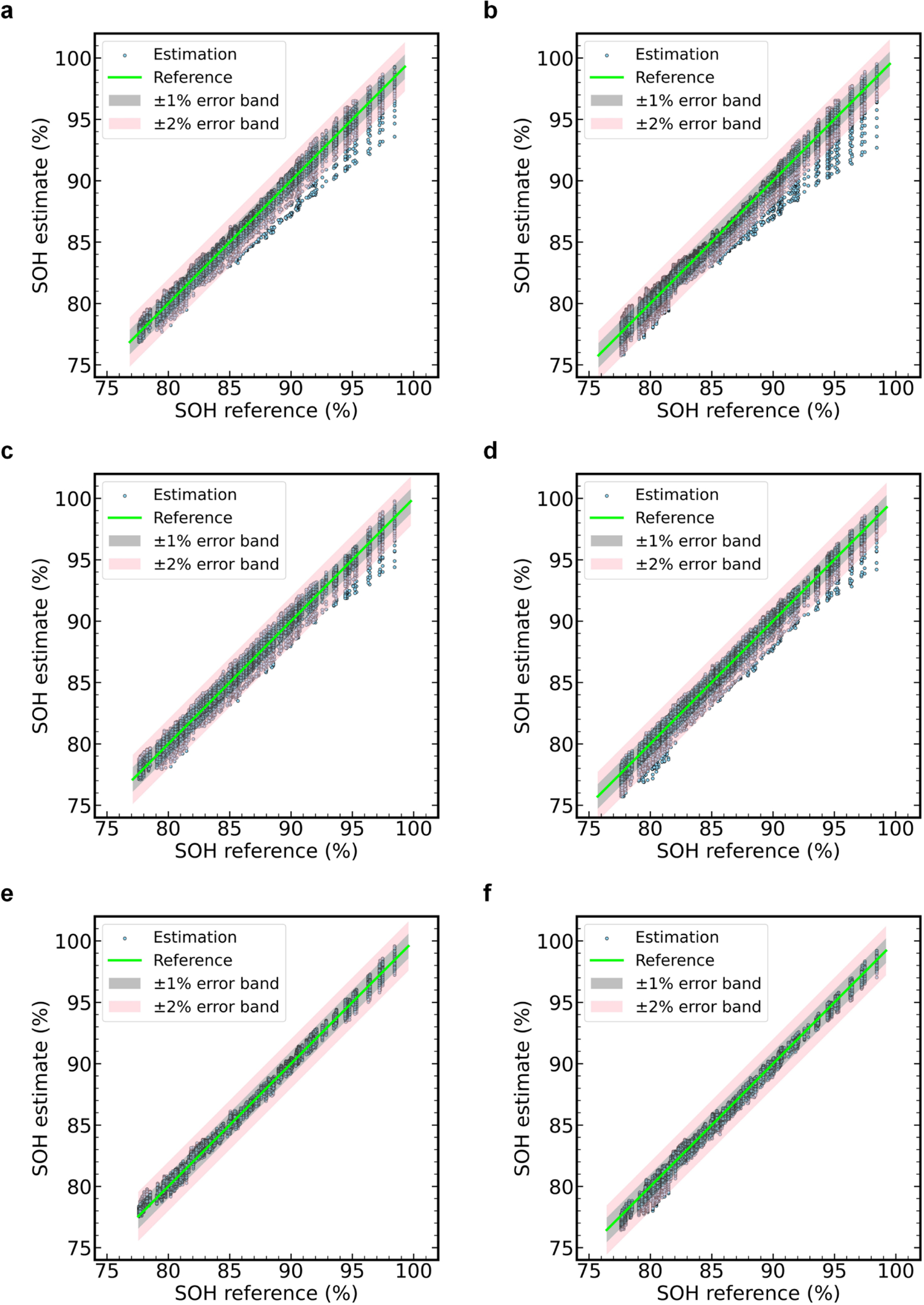
To further illustrate the detailed pattern of the SOH estimation results, the estimation values are depicted as a function of the reference values in Fig. 13, represented by discrete points. Here, the green line denotes the ideal estimation reference without any errors. The grey region represents the ±1% error band, and the pink region denotes the ±2% error band. For the direct learning of FNN (Fig. 13a), most of the estimation errors can be controlled within the ±2% error band for SOH below 90%. However, a certain part of the results shows an obvious underestimation as SOH further surpasses 90%. As for the transfer learning of FNN (Fig. 13b), the estimation distribution is similar to that of the direct learning. However, the underestimation becomes more striking as SOH exceeds 85%. This means the FNN model tends to cause larger SOH estimation error or uncertainty for new batteries. For CNN (Figs. 13c and 13d), the estimation performance seems more stable compared with FNN (Figs. 13a and 13b). The underestimation is not obvious except when the SOH exceeds 95%. Moreover, the transfer learning of CNN just exhibits slight weakening compared to the direct learning. As for LSTM (Figs. 13e and 13f), it shows an excellent SOH estimation performance during the whole battery life cycle for both the direct and transfer learning scenarios. Most of the estimation errors fall within the ±1% error band, with minor underestimation observed only at the initial and final stages of the battery life cycle. Similarly, the direct learning still shows a minor advantage over the transfer learning especially at the end stage of the battery life cycle.

Figure 13. Plots of SOH estimation results as a function of the reference values to highlight the deviation of the estimation from the references for (a) FNN-direct learning, (b) FNN-transfer learning, (c) CNN-direct learning, (d) CNN-transfer learning, (e) LSTM-direct learning and (f) LSTM-transfer learning.
Download figure:
Standard image High-resolution imageFigure 14 presents the relationship between the battery SOH and the number of cycles. The experimental SOH is represented by the black line and points, while the scope of the estimation results for each SOH value are depicted by blue error bars. Similar to Fig. 13, the grey region corresponds to the ±1% error band, and the pink region represents the ±2% error band. Overall, the tested battery cell undergoes 385 cycles throughout its entire lifespan, and the SOH exhibits a degradation trend with fluctuations as the cycle number increases. For the FNN model (Figs. 14a and 14b), the SOH is generally underestimated until approximately 220 cycles, and the maximum estimation error exceeds 2% prior to around 110 cycles. However, once after 220 cycles, the estimation results predominantly fall within the ±1% error band. For CNN (Figs. 14c and 14d), the estimated SOH results exhibit a relatively consistent pattern throughout the battery's lifespan. However, the SOH is generally underestimated for most of the cycles, particularly in the transfer learning scenario. In the case of LSTM (Figs. 14e and 14f), the SOH estimation results are concentrated within the ±1% error band, while the worst estimation results in the transfer learning scenario display an error close to −2% after 280 cycles. In summary, the LSTM model outperforms the FNN and CNN models, and the CNN model shows a more uniform distribution with respect to the estimation error compared to the FNN model. Additionally, all three models experience a slight decline in performance under the transfer learning scenario compared to the direct learning scenario.

Figure 14. Plots of SOH values as a function of cycle numbers, with the scope of the estimation results depicted by blue error bars: (a) FNN-direct learning, (b) FNN-transfer learning, (c) CNN-direct learning, (d) CNN-transfer learning, (e) LSTM-direct learning and (f) LSTM-transfer learning.
Download figure:
Standard image High-resolution imageOverall, according to the above comparative study, the LSTM-based deep learning model exhibits outstanding SOH estimation performance in both the simple direct learning and complex transfer learning scenarios. Moreover, it should be noted that, the input segment of the present models is just limited to a small voltage span (0.29 V) during the CC charging process. This means it just requires a short charging data segment to realize the real-time and reasonable SOH estimation. Specifically, the time required for most of the charging data segments will not exceed 20 min (Fig. 15a), especially in the early charging stage which just needs about 10 min to realize the estimation with a high accuracy (Figs. 13f and 15a). Accordingly, the required charging capacity (ΔSOC) for most of the data segments is below 30% (Fig. 15b), especially in the early charging stage which just needs around 13% and 19% ΔSOC to realize the estimation for aged and new batteries, respectively.

Figure 15. (a) Charging time and (b) charging capacity (ΔSOC) required for charging data segment acquisition (SOH estimation) when SOH = 95% and SOH = 85%.
Download figure:
Standard image High-resolution image
Conclusions
We developed three deep learning models based on the FNN, CNN, and LSTM frameworks to investigate their potential for online SOH estimation of Li-ion batteries using partial and random charging data segments. The results indicate that the LSTM model outperforms other models, and it shows the maximum error of 1.53% and 2.19% and the average error as low as 0.28% and 0.30% over the test set in the direct learning and transfer learning scenarios, respectively. Comparatively, the CNN and FNN models exhibit slightly inferior performance, particularly in the complex transfer learning scenario. Compared with the direct learning scenario, the models used in the transfer learning scenario generally demonstrates a degradation in performance due to significant difference in features between the training and test sets. However, the LSTM model still exhibits great transfer learning capability with an average error of 0.30%, compared to 0.43% for CNN and 0.48% for FNN. Notably, our study highlights that real-time and reasonable SOH estimation can be achieved with a short online charging data segment, typically around 10 min for the initial charging stage and no more than 20 min for the majority of the charging process.
Our work provides a comprehensive evaluation of online SOH estimation for Li-ion batteries using three deep learning models throughout the battery's entire life cycle. Furthermore, we demonstrate the feasibility of its practical implementation in EVs by considering the flexibility of the input segment range and the robustness of complex transfer learning performance. However, it is important to highlight that the potential of present models in overcharging scenarios has not been evaluated, primarily due to the absence of overcharging data in the experimental dataset. In our forthcoming research, we aim to extend our study to include overcharging scenarios, thereby broadening the scope of applicability for deep learning-based estimation methodologies within a more extensive range of engineering-oriented contexts.
Acknowledgments
This work was supported by the National Key R&D Program of China (Grant No. 2022YFE0208000), the Shanghai Key Laboratory of Aerodynamics and Thermal Environment Simulation for Ground Vehicles (Grant No. 23DZ2229029), and the Shanghai Automotive Wind Tunnel Technical Service Platform (Grant No. 19DZ2290400) and the Fundamental Research Funds for the Central Universities. N.M. gratefully acknowledges the support of the International Institute for Carbon Neutral Energy Research, sponsored by the Japanese Ministry of Education, Culture, Sports, Science and Technology.