
Abstract
A high-resolution, 3D, computational fluid dynamics (CFD) model was developed and implemented for simulating the heat and gas generation during thermal runaway failure of an 18650 Li-ion battery cell. The model accounts for volumetric gas generation within the active material of the cell and for gas flow through the jellyroll, into the headspace regions, through the safety vent, and out into the surrounding air space. The simulation captures the key features of the oven test, including: self-heating from decomposition reactions, initial venting (i.e. blowdown), temperature decrease due to evaporative cooling, thermal runaway, a second venting event associated with thermal runaway, and cooldown. The highly detailed geometric model of the safety vent allowed for new insight into the physics of venting during thermal runaway. Secondary flows, including ring vortices, counter-rotating vortex pairs, and corner vortices, were found to increase the rate of mixing of the vented gases with the surrounding air. The simulation was compared to previously reported experimental results and found to have good qualitative agreement of jet flow direction. The present thermal abuse model forms the basis for future studies to consider the role of gas impingement heat transfer and gas combustion in full battery pack propagating failures.
Highlights
A 3D thermal abuse model was implemented for an 18650 li-ion cell oven test
Model includes gas generation from decomposition reactions and evaporation
Simulations show gas flow through the jellyroll, safety vent, and out of the cell
Spatial distribution of vented gases depends strongly on rate of gas generation
Turbulent flow structures increased the vent gas mixing rate with surrounding air
Export citation and abstract BibTeX RIS

Original content from this work may be used under the terms of the Creative Commons Attribution Non-Commercial No Derivatives 4.0 International licence. Any further distribution of this work must maintain attribution to the author(s) and the title of the work, journal citation and DOI.
List of Symbols
| A | Frequency factor |
| b | Spreading parameter for melting model |
| Co | Courant number |

| Specific energy 
|
| Ea | Activation energy |

| Body force vector |

| Gravity vector |
| Gk | Turbulence production due to mean velocity gradients |
| Gb | Turbulence production due to buoyancy |

| Specific enthalpy |

| Flux of ith species due to molecular, turbulent, and thermal diffusion |
| k | Turbulent kinetic energy; thermal conductivity |
| kb | Boltzman constant |

| Turbulent thermal conductivity |

| Porous material permeability tensor |

| Volumetric mass generation rate |
| mv | Mass of electrolyte vapor |
| n | Reaction order |
| p | Static pressure |
| Pv | Saturation vapor pressure |

| Volumetric heat generation rate |
| R | Reaction rate |
| Ri | Source term of the ith species due to reactions |
| Rs | Specific gas constant |

| Turbulent dissipation rate source term |

| General scalar source term |
| Sh | Heat source term |
| Si | Source term for the ith species |
| Sk | Turbulent kinetic energy source term |
| Sm | Mass source term |
| t | Time |
| T | Temperature |
| Tmelt | Melting temperature |

| Velocity vector |
| Vh | Headspace volume |
| Vjr | Volume of jellyroll |
| x | Non-dimensional degree of reaction conversion; non-dimensional species concentration |
| Yi | Mass fraction of the ith species |
| YM | Turbulence dissipation from fluctuating dilatation |
| Z | Compressibility factor |

| Liquid fraction for melting model |

| Diffusion coefficient |

| Turbulent diffusion coefficient |

| Enthalpy of reaction for a given decomposition reaction |

| Heat of fusion in melting model |

| Heat of vaporization in evaporation model |

| Mass of vent gas generated from a given decomposition reaction |

| Turbulent dissipation rate |

| Density |

| Molecular viscosity |

| Turbulent viscosity |

| Dynamic viscosity |

| Turbulent Prandtl number for turbulent kinetic energy |

| Turbulent Prandtl number for turbulent dissipation rate |

| Stress tensor |

| Turbulent stress tensor |

| General scalar field variable |
When Li-ion battery cells are subjected to abuse conditions, heat and gas are generated as a result of decomposition reactions which occur at elevated temperatures. 1 The heat accumulation within the cell will accelerate the reactions, resulting in thermal runaway if the heat generation rate exceeds the rate of heat removal. In addition, evolved gases will raise the internal pressure of the cell, eventually leading to a breach of the pouch or casing material. 1 Cells with metallic casings are typically designed with a pressure-relief vent mechanism to avoid over-pressurization and energetic failure of the casing. However, the release of flammable gases into the surrounding space creates a dangerous condition and may lead to fire or explosion.
The resulting combustion of vented materials plays a significant role in thermal runaway propagation in battery modules. Experiments have shown that fire will pre-heat neighboring cells, accelerating the pace of thermal runaway propagation in modules. 2 The importance of capturing these heat transfer processes is also highlighted in a recent study which used the fractional calorimetry technique to measure the distribution of energy released from a single cell failure. 3 The study showed that approximately 30% of the total energy released was conducted away from the cell casing while 70% of the total energy release was external to the cell. 3 The two major contributions to the vented energy are the sensible heat of ejecta and the chemical energy released during combustion of vented gases. This finding suggests that propagation models which are based only on conduction heat transfer may suffer large deviations with experimental measurements. For instance, if the total energy obtained from calorimetry experiments is used in a heat-conduction-based thermal abuse simulation, then heat transferred to neighboring cells would be over-predicted. Coman et al. have accounted for this effect by applying an efficiency factor to the heat generation terms of the thermal abuse model to reduce the amount of cell-to-cell heat conduction. 4
Despite the role of fire on accelerated propagation rate, relatively few studies have captured the complex fluid dynamic and heat transfer phenomena involved in venting and combustion. Incorporating the heating load due to combustion into existing, heat-conduction-based propagation models would require consideration of the mixing of gases and vapors with surrounding air. Differences in geometry and air circulation within various module and battery pack designs will create different conditions for combustion. As a result, bulk total heat release measurements will not provide inputs to models that are adaptable to a variety of scenarios. This variation is illustrated by an almost order of magnitude greater total energy release 5 measured in oxygen rich cone calorimetry experiments than in oxygen constrained fractional calorimetry experiments. 3 Thus, there is a need to develop fluid-dynamics-based models which can capture the venting process and the mixing of flammable gases with air prior to combustion. The heating effects from combustion could then be simulated with accuracy in a variety of battery pack or module geometries. Further, in scenarios where combustion of gases occurs prior to exiting the cell, the impingement heat transfer problem will also be strongly dependent on turbulent mixing. The heat transfer rate depends directly on the difference in temperature between the wall and the impinging gases. 6 Mixing of hot vent gases with surrounding, cooler air will reduce the driving temperature difference for convection.
Previous models have considered venting and combustion but fail to capture the spatial dependence of the vented gases caused by the complex safety vent and cell cap geometry. Coman et al. 7 used a 0-D, lumped capacitance formulation to model thermal runaway of 18650 format cells. Their model included the effects of gases generated by decomposition reactions and by electrolyte evaporation during prior to the point of vent-activation. In previous work, our group extended the model to include electrolyte evaporation after vent-activation and found that heat absorbed by evaporation plays a significant role in the time-to-runaway. 8 While fast and computationally inexpensive, 0-D models are unable to simulate the distribution of gases vented from the cell into the surrounding space. To quantify the structure of the vented gas flow field, our group also conducted a 3D, steady-state CFD analysis of gases emerging from four commercial 18650 cells using a hybrid RANS/LES turbulence model and a detailed geometric representation of the safety vent. 9 It was found that the safety vent structure influences key flow parameters, such as: maximum Mach number, location of choke point, trajectory of jets emerging from the vent, and degree of turbulent mixing. Another simulation using stationary boundary conditions was conducted recently by Cellier et al. 10 The authors implemented a detailed combustion model with LES turbulence model to study the flame structure emerging from an 18650 cell having 3 or 5 vent holes showing that increased flow velocity for the 3-hole vent resulted in the flame lifting away from the cell casing.
Mishra et al. 11 considered the effects of venting flow on thermal runaway propagation using a 3D computational fluid dynamics model. The model considered the hot gases ejected from a circular opening in the top or sidewall of a cell. Kim et al. 12 developed a 2D axisymmetric model, including venting and gas phase reactions for an 18650 cell at various states of charge. Kong et al. 13 used the 2D axisymmetric approach to model venting and combustion for a circular venting opening but simplified the thermal runaway model to a 0-D lumped approach. Where Kim et al. 12 used a single, global reaction mechanism for heat and gas generation, Zhao et al. 14 considered individual gas generation reactions for H2, C2H4, CH4, CO, CO2, H2O, and O2. And, the safety vent at the positive terminal was modified to create a circular opening and the simulations used a 2D axisymmetric framework. 14 Wang et al. 15 used a concept similar to Kong et al. 13 to develop a coupled thermal resistance network and CFD-based venting model implemented on a module of prismatic cells. Thermal propagation was solved using the thermal resistance network, while venting and spread of flammable gases from a rectangular opening was quantified with and without air ventilation. And, Wang et al. 16 extended the analysis to include a dispersed phase model to track the distribution of solid ejecta during and after venting.
The present work builds on the previous literature by developing a comprehensive 3D fluid-dynamics-based Li-ion 18650 cell thermal abuse model incorporating the detailed geometry of the cell. The model accounts for heat generation from decomposition reactions, electrolyte evaporation, and venting of vapors and decomposition products. In contrast with the stationary boundary conditions of Refs. 9, 10, the present work considers the entire thermal runaway process as a dynamic process with internal gas generation and venting. In contrast with Refs. 11–16, the present work includes a detailed geometric representation of the safety vent which allows for simulation of the complex jet structure and spatial distribution of vented gases emerging from the cell. Finally, the present work is distinguished from prior literature through a detailed analysis of the turbulent flow structures observed during venting which play a key role in mixing of vented gases with the surrounding air. The key features of the model and the implementation into a commercial, computational fluid dynamics (CFD) software is described. Qualitative comparisons between simulations and experiments of previous studies are conducted, and new insights into the physics of venting are discussed. This work aims to provide a foundation for future studies that investigate the spatially-dependent heat load on neighboring cells from impingement and ignition of vented gases.
Methods
The thermal abuse and venting model is based on a commercially-available CFD software (Ansys® Academic Research FLUENT, Release 2019/R3). 17,18 The software uses the finite volume method to discretize the governing PDEs into algebraic equations. The governing equations for a three-dimensional flow begin with the Reynolds-Averaged Navier–Stokes equations for continuity and momentum transport:


Flows involving heat transfer and/or compressibility effects must include the energy transport equation:
In addition, turbulent flows must include additional transport equations for scalars such as turbulent kinetic energy (k) and turbulent dissipation rate( ):
):
where C1,  C2, and
  are model constants. Problems involving mixing of multiple gas-phase species must also include species transport equations (N-1 additional PDEs where N is the number of species). Below, the transport equation for the mass fraction of ith species, Yi
, is:
are model constants. Problems involving mixing of multiple gas-phase species must also include species transport equations (N-1 additional PDEs where N is the number of species). Below, the transport equation for the mass fraction of ith species, Yi
, is:

In solid and stationary regions, the energy equation is the only governing equation, which reduces to:

The thermal abuse simulations considered herein contain all of the aforementioned physics and governing equations. These governing equations are considered the standard CFD solver upon which the present work is based. 17,18
Scalar transport equation for reactions
The standard CFD solver was customized to add functionality needed for the thermal abuse and venting model. Because the thermal abuse model includes exothermic chemical reactions within the active material of the battery cell, a modification to the standard CFD solver was necessary to track the progress of these reactions. The generic transport equation for scalar,  is:
is:

The scalar transport equation was modified to solve the ordinary differential equations (ODE) which govern the reaction kinetics. As an example, consider the following, first-order reaction with Arrhenius-rate kinetics:

where x may represent a non-dimensional species concentration or non-dimensional degree of reaction conversion, A is the frequency factor, Ea is the activation energy, kb is the Boltzman constant, T is absolute temperature, and n is the reaction order. In order to use the scalar transport equation (Eq. 8) to track the progress of a chemical reaction (Eq. 9), several modifications are needed. First, the advective flux term (second term on left side) is disabled within the user interface of the software. Second, the diffusive flux term (first term on right side) is disabled by setting the diffusion coefficient to zero, Γ = 0, which results in ΓT = 0. Finally, it is convenient to modify the transient term by dividing both sides by the density, ρ. With these modifications, Eq. 8 reduces to the following equation, which has the same form as Eq. 9:

Thermal abuse model
The thermal abuse model used in this work is based on a well-known model that has been developed previously. 19–22 The thermal abuse model considers four, exothermic chemical reactions which were originally developed for an LCO/graphite chemistry, but can be adapted to simulate other cell chemistries. 23 The reactions are: decomposition of metastable species in the SEI-layer (abbr. SEI-d), reaction of intercalated lithium in the anode with electrolyte solvent which leads to formation of new SEI-layer (abbr. SEI-r), decomposition of electrolyte (abbr. elec), and reaction of cathode with electrolyte solvent (abbr. cat). Because the SEI-r reaction involves formation of new SEI layer, an ODE is used to track the thickness of the SEI layer (abbr. tSEI) as the SEI-r reaction progresses. The anode-side reaction mechanisms and kinetic parameters were originally proposed by Richard and Dahn 19 and implemented by Hatchard et al. 21 The same mechanism and kinetic parameters for the anode-side reactions are adopted here. The cathode-side reaction mechanism was proposed by MacNeil and Dahn 20 and the kinetic parameters implemented by Hatchard et al. 21 for this mechanism were adopted here. One change was made to the cathode reaction, whereby the frequency factor was reduced by a factor of 1.2 to obtain better agreement with experimental data, as discussed in the Electronic Supplemental Information. The reaction mechanism for electrolyte decomposition was proposed by Spotnitz and Franklin 22 and the kinetic parameters implemented by Kim et al. 24 for this mechanism were adopted here. A summary of the reactions, equations, and initial conditions are shown in Table I.
Table I. Reaction Mechanisms and Kinetic Parameters used in the Present Work.
| Reaction Abbr. | Initial Condition | ODE used in Eq. 10 for each Reaction | References |
|---|---|---|---|
| SEI-d | xf = 0.015 |
| 19, 21 |
| SEI-r | xi = 0.75 |
| 19, 21 |
| tSEI | tSEI = 0.033 |

| 19, 21 |
| elec | celec = 1 |
| 22, 24 |
| cat | αcat = 0.04 |
| 20, 22 a |
a)Frequency factor in the cathode decomposition reaction was reduced by a factor of 1.2 for improved fit with experimental data as shown in the Electronic Supplementary Material.
Volumetric heat and gas generation
Heat and gas are generated, volumetrically, throughout the active material as the decomposition reactions progress. During each iteration of the solution procedure, the volumetric heat generation follows:

where Δh is the enthalpy of reaction, m is the initial mass of reactants (total amount within the cell), R is the reaction rate, and Vjr is the volume of the jellyroll (or the volume of the active material if the format is not cylindrical). This volumetric heat is applied as a source term in the energy equation within the jellyroll region, Eq. 7. The same concept is used for volumetric gas generation:

where Δm is the mass of vent gas generated by a given reaction. The volumetric mass generation is applied as a mass source term (Eq. 1.) and species source term (Eq. 6) within the jellyroll.
It was assumed that each decomposition reaction produced a mixture of gases (i.e. "vent gas") where the vent gas composition is the same for each decomposition reaction. It was also assumed that the electrolyte vapor within the cell was primarily dimethyl carbonate. 7 Therefore, there were N = 3 gas-phase species considered in the present work: vent gas, electrolyte vapor, and air. There were also N—1 = 2 species transport equations: vent gas and electrolyte vapor. The local mass fraction of air is calculated as unity minus the sum of the mass fraction of vent gas and electrolyte vapor.
Table II shows parameters which define the heat and mass generated for each reaction. Heat generation parameters in Table II were adopted from previous work. 19–22,24 The mass generation amounts, on the other hand, were unknown and required estimation. To obtain a reasonable estimate, a sensitivity analysis was performed to investigate the effect of assigning mass generation to each decomposition reaction. The sensitivity analysis and discussion justifying the final model parameters are presented in the Electronic Supplemental Information.
Table II. Heat and Mass Generation Parameters for each Reaction.
| Rxn. | Heat Generation | Mass Generation | |
|---|---|---|---|
| Δh (J g−1) | m a) (g) | ∆m b) (g) | |
| SEId | 257 19,21 | 8.08 24 | 0 [est.] |
| SEIr | 1714 19,21 | 8.08 24 | 0 [est.] |
| elec | 155 22,24 | 5.38 24 | 6 [est.] |
| cat | 314 20,21 | 16.16 24 | 0.017 [est.] |
a)Mass of reactants for heat generation, m, were calculated using the specific material content (g/m3) from reference 24 multiplied by the jellyroll volume (m3) of the present model. b)A sensitivity analysis, presented in the Electronic Supplementary Information, was conducted to estimate the mass of gas generation assigned to each reaction, Δm.
Gas flow within the cell and external to the cell
The present work considers a single, small format, 18650 Li-ion cell shown in Fig. 1. It is assumed that evolved gases travel more readily along the in-plane directions of the electrode stack, axially, and circumferentially, in any direction towards or away from the cell header as illustrated by the arrows in Fig. 1a. In contrast, gases do not travel easily in the radial direction due to the presence of the current collectors. Because the electrode stack is spirally wound, however, flow of gases in the circumferential direction will result in some flow in the radial direction. The various components (current collector, burst disk, and positive terminal) of the cap are represented in detail for gas to flow through from the inside of the cell and into the surrounding space. A zoomed-in view of the header and positive terminal assembly is shown in Fig. 1b, where different components are labeled.

Figure 1. Modeling strategy for capturing the flow physics of venting: schematic of 18650 format cell with gases travelling within the jellyroll, into the headspace, and through the vent (a); zoomed-in view of positive terminal assembly (b); schematic of gas channels within the electrode layer, resulting in flow which is aligned with the in-plane direction (c); and, schematic of solution strategy (d).
Download figure:
Standard image High-resolution imagePorosity, permeability, and thermal conductivity of the jellyroll
The different cell components labeled in Fig. 1b consist of solid, fluid, and porous-fluid zones. The positive terminal, burst disk, current collector, gasket, insulating ring, and case are solid zones. The headspace is a fluid zone consisting of a gas-phase mixture of electrolyte vapors and products of decomposition reactions. The jellyroll is considered to be a porous zone which is partially solid and partially fluid. The solid portion is modeled using thermophysical properties of the electrolyte-soaked jellyroll. The fluid portion is modeled as a gaseous phase. The concept is illustrated in Fig. 1c. The gas-phase porosity consists of small channels between electrode-separator layers. The current collectors are assumed to be impermeable and the resulting flow path for the evolved gases is aligned with the in-plane direction of the electrode layers. Therefore, the permeability of the jellyroll region, like thermal conductivity, is strongly anisotropic.
The gas-phase porosity and permeability are assumed to be anisotropic and constant throughout the thermal runaway event. Porosity for the gas phase was estimated by assuming that the sum of the thickness of the two gas channels is 2.0% the thickness of the electrode stack corresponding to two gas channels, each having height of 2 μm, within a 200 μm thick electrode stack. The gas-phase porosity is, therefore, estimated to be 2.0%.
The permeability of the jellyroll affects the resistance to the gas flow within the porous medium. The resistance to flow in a porous medium may be modeled using Darcy's law:

where  is the pressure gradient,
  is the velocity vector, μ is dynamic viscosity and
  is the second order permeability tensor. The cylindrical anisotropic permeability is:

where Kr
is the radial permeability, Kt
is the tangential permeability, Kz
is the axial permeability, and Kθ
is a parameter calculated locally depending on the position of the mesh element. Thermal conductivity of the jellyroll was also considered to be cylindrically anisotropic and was modeled using the same second order tensor as Eq. 14, but replacing permeability components, K, with conductivity components, k. The radial thermal conductivity was assumed to be kr
= 0.4 W/(m K), tangential thermal conductivity was kt
= 20 W/(mK), and axial thermal conductivity was kz
= 20 W/(mK).
K), tangential thermal conductivity was kt
= 20 W/(mK), and axial thermal conductivity was kz
= 20 W/(mK).
Because the gas-phase channels are very small, the Reynolds number of the gas phase flow within the jellyroll is assumed to be in the laminar regime. Under this assumption, permeability was calculated using the analytical solution for Poiseuille flow, a scenario where laminar flow between parallel plates is driven by pressure differential. The Poiseuille flow permeability is K = h2/12, where h is the summed height of the two parallel gas channels, 4 μm. The resulting permeability in the axial and circumferential directions was Kz = Kt = 1.33 × 10⁻¹² m2. The permeability in the radial direction, Kr , was assumed to be two orders of magnitude lower. The layered jellyroll, modeled as a porous medium with anisotropic permeability, was chosen because the focus of the present work was to investigate the 3D physics of venting during blowdown (immediately after vent-activation), during non-VLE evaporation, and in the moments leading up to full thermal runaway, as shown in Fig. 1b for an oven test scenario. Prior to full thermal runaway, the internal cell temperatures are relatively low, below the melting point of the current collector foils. High-speed radiography has shown that the layered jellyroll structure directs debris between the layers until the point at which the current collectors begin to melt. 25 Once the local jellyroll temperature exceeds the melting point of the current collectors, the jellyroll breaks down and becomes fluidized as globules form and become entrained in gases leaving the cell. 25 Once fluidization occurs, the layered jellyroll structure breaks down and permeability may be considered isotropic. 12 Future models may consider the transition from anisotropic to isotropic permeability and an increase in porosity associated with fluidization of the jellyroll.
Electrolyte evaporation
A model for evaporation of liquid electrolyte before and after vent-activation was developed previously and adopted for the present work. 8 When the vent is closed, the electrolyte is in liquid-vapor equilibrium. The vapor pressure within the headspace region is equal to the saturation vapor pressure. The mass of electrolyte vapor in the headspace at a given instant is calculated using the equation of state:

where Pv
is the saturation vapor pressure of the electrolyte, Vh
is the headspace volume, Rs is the specific gas constant,  is the volume-averaged temperature of the jellyroll and headspace zones, and Z is the compressibility factor. The headspace volume, Vh
, is the sum of the headspace zone and the gas-phase volume of the jellyroll. The volumetric generation of electrolyte vapor in the jellyroll volume is calculated as:
is the volume-averaged temperature of the jellyroll and headspace zones, and Z is the compressibility factor. The headspace volume, Vh
, is the sum of the headspace zone and the gas-phase volume of the jellyroll. The volumetric generation of electrolyte vapor in the jellyroll volume is calculated as:

where the overbar on the time-rate-of-change of temperature designates the volume-averaged value of the jellyroll and headspace zones. The partial derivative of the mass of electrolyte vapor with respect to temperature is:

where, again, the overbars designate volume-averaged values. The mass generation of electrolyte vapor, from Eq. 16, was applied as a mass source term in Eq. 1 and as a species mass fraction source term in Eq. 6.
A polynomial function for vent-activation pressure as a function of temperature was adopted from previous work 26 and is defined in the Electronic Supplementary Information. After internal pressure exceeds the vent-activation pressure, free electrolyte which is not bound in the pores of the separators and electrodes will evaporate at a constant rate. This is known as the constant rate drying period (CRDP). Second, the remaining bound electrolyte will evaporate at a decreasing rate. As the jellyroll dries out, the evaporation rate decreases with decreasing electrolyte concentration. This is known as the decaying rate drying period (DRDP). The transition between CRDP and DRDP occurs when the free electrolyte is depleted at time t = tdryout . The evaporation rate is defined as:
where K1 , K2 , K3 are constants, ml is the mass of liquid electrolyte remaining, ml0 is the initial liquid electrolyte in the cell, and ml,free is the amount of free electrolyte. The evaporation parameters were: K1 = K2 = 10 mg s−1, K3 = 0.0045 s−1. The initial amount of electrolyte is the same as used in the heat generation model, ml0 = melec = 5.38 g. The free electrolyte was ml,free = 0.25 g. Identification of evaporation parameters is discussed in the Electronic Supplementary Information. A heat source term was included in Eq. 7 to account for the latent heat:

where Δhv is the specific heat of vaporization.
Melting and solidification
Melting and solidification of the separator was included in the thermal abuse model. A sigmoid function was assumed for the liquid fraction of separator as a function of temperature:

where Tmelt is the melting temperature and b is a spreading parameter. For separator melting in the present work, Tmelt was 130 °C and b was 0.35. 8 After each iteration of the solution procedure, the time-rate-of-change of liquid fraction was calculated within each cell of the jellyroll zone. A heat source term was included in Eq. 7 to account for the latent heat:

where Δhf is the specific heat of fusion and ms is the mass of the separator.
Model Setup and Solution Procedure
Standard numerical schemes commonly employed for CFD analysis are used in the present work. 17,18 The discretization schemes were: second-order implicit time-stepping, second order upwind differencing for advective terms, and central differencing for diffusive terms. The pressure-based solver was used in favor of the density-based solver for improved numerical stability. 17,18 Two algorithms were used, during different periods of the simulation, for pressure-velocity coupling. Prior to venting, the semi-implicit pressure linked equations (SIMPLE) algorithm was used with a segregated solver. After the vent opens, the coupled solver was used for improved numerical stability at the expense of greater memory requirement. 17,18 The two-equation, realizable k-epsilon turbulence model with scalable wall function model was chosen for its ability to accommodate a computational mesh with large changes in first cell layer height. 17,18
Commercial Li-ion cell geometry
The present simulations were conducted using the cell geometry for an LG INR18650 MJ1 cell. The detailed geometry of the positive terminal assembly, in the vent-activated state, was obtained in previous work. 26 The positive terminal assembly was isolated from the cell, pressurized so that the vent mechanism was activated, and then scanned using an industrial X-ray apparatus. The resulting computed tomography (CT) scans were used to develop a highly detailed 3D geometric model for use in numerical simulations such as the present CFD study. Detail of the 3D positive terminal assembly is shown in Fig. 1b. CT scans of commercial cells, including the LG MJ1, are publicly available for download. 27–30
Solution strategies
Several solution strategies were implemented to reduce computational expense while still capturing the relevant physical processes occurring across a wide range of length and time scales. These strategies were devised based on the previously reported progression of thermal runaway for an oven test scenario shown in Fig. 1d. 21 During initial heating phase indicated in Fig. 1d, the cell is heated by convection and radiation heat transfer. Internal heat and gas generation from decomposition reactions are progressing at a low rate, so the headspace and jellyroll were both set to solid zones. Even though these volumes were set as solids, evaporation and vent gas generation processes were still calculated within custom C-code which executes in tandem with the standard CFD solver. In this manner, the effects of gas generation and pressure buildup were still manifest in the model. Figure 1d shows a rapid decrease in cell pressure as gas vents from the cell immediately following vent activation. To capture the highly transient blowdown process, the solution was paused while the state of the model was changed. The vent plane was changed from a wall to an interior surface. The jellyroll zone was changed from solid to porous zone, and the headspace was changed from solid to a fluid zone. In this way, after restarting the CFD solver, flow begins venting from the cell.
Another strategy to save computational expense was the use of adjustable time step, as illustrated in Fig. 1d. In this thermal abuse scenario, there are two highly transient processes. First, there is a rapid drop in internal pressure at the moment of vent-activation as gases rush out of the cell and expand into the surroundings. To capture this blowdown event, the time step size set to 0.1 μs concurrently with changing the vent plane from wall to interior surface. Second, there is a sharp temperature increase at the moment of thermal runaway. To capture the rapid thermal runaway process, the rate of change of the field variables was used as a feedback signal to adjust the time step (reaction progress variables and cell temperature). In the present work, the pressure and velocity fields were not used to modulate the time step but could be implemented in future CFD-based models. Finally, as mentioned previously, different numerical schemes were used during different phases of the thermal abuse simulation. During the initial heating phase, prior to initial venting, the segregated pressure-based solver with SIMPLE algorithm was used to reduce computational expense. 17,18 When the vent opens, the coupled solver was used for increased numerical stability. 17,18
The pressure-based, coupled solver is robust for a wide range of local flow Courant numbers (whereas density-based solver with explicit time integration is subject to the unity Courant number requirement). The maximum local Courant number varies throughout the thermal runaway simulation but may be estimated using conservative values of velocity scale of 800 m s−1 (based on isentropic flow equations for an internal pressure of 1.5 MPa upstream of the choke point), mesh length scale of 80 μm (based on mesh size around the safety vent), and time step of 0.1 μs (based on the time step at the moment of initial venting). These values resulting in an estimated Courant number of Co ≈ 10 during the highly transient blowdown process.
Mesh and boundary conditions
The computational domain and boundary conditions are shown in Fig. 2a. The 18650 cell was located coaxially within a cylindrical chamber having diameter of 0.1 m and subjected to a thermal abuse scenario consisting of hot air at a temperature of 155 °C flowing past the cell. The incoming air speed was 0.6 m s−1 which resulted in an average convective coefficient on the surface of the cell equal to 7 Wm−2K−1. The outlet of the chamber was set to zero gauge pressure. The wall of the chamber was set to a constant temperature of 155 °C. Radiation heat transfer was computed using the surface-to-surface method, to account for heat transfer between the cell surface and the chamber wall.
17,18
The chamber wall was assumed to be a black surface while the cell case and positive terminals were assumed to be gray surfaces with emissivity of 0.8.

Figure 2. Computational domain and boundary conditions (a), x-normal slice showing mesh detail (b), and z-normal slice showing mesh detail (c).
Download figure:
Standard image High-resolution imageThe computational mesh contained a combination of hexahedral and polyhedral elements. For regions with simple geometry (i.e., jellyroll, mandrel, and parts of the cell case) hexahedral elements were used. All other regions were meshed using polyhedral elements which reduces the total element count and improves numerical efficiency relative to tetrahedrons. 17,18 The global mesh size constraints were: maximum element size of 7 mm, minimum element size of 80 μm, and growth rate of 1.2. The length scale of the mesh elements in and around the safety vent was 80 μm with some local refinements as small as 25 μm to capture small features and to improve orthogonal quality. Boundary layer refinement was included on all wall surfaces using 5 layers with transition ratio of 0.272. The total element count was approximately 5.02 million with minimum orthogonal quality of 0.103. Figure 2b shows a cross section of the mesh in the x-normal direction and Fig. 2c shows a cross section of the mesh in the z-normal direction. In Figs. 2b, 2c, the highly detailed vent cap geometry is shown.
The CFD component of the present model was validated in a previous study by comparing discharge coefficients with experimental values. 9 In comparison with the present work, validation simulations were conducted with the same geometric model of the safety vent assembly, same mesh size constraints and mesh type, and same solver settings with the only difference being steady RANS solver in the validation study and unsteady RANS solver in the present work. Simulated discharge coefficients agreed well with experiments across a range of pressure ratios. Additionally, the local flowfield structure was validated by comparing simulations with experiments for a sharp-edge orifice. 9 The simulated shock cell length was in good agreement with experimental values.
Results and Discussion
A thermal abuse simulation was carried out at an inlet temperature of 155 °C. The CFD-based thermal abuse model captures the effects of internal gas generation and venting in addition to the heat generated by decomposition reactions. The following sections include data and discussion related to: the evolution of temperature, internal pressure, and reactant species within the cell; evaporative cooling and venting flow physics during initial venting; the progression into thermal runaway and second venting event; and analysis of the turbulent flowfield and identification of large scale flow structures.
Bulk temperature and gas evolution comparison: 3D Model, previously developed 0-D model, and experiments
Figure 3a shows the jellyroll temperature vs time comparing the 3D model results with the experiments of Hatchard et al. 21 and with a 0-D model. Hatchard et al. 21 conducted an oven test on an 18650 LCO/graphite cell. The initial temperature was 28 °C and the oven temperature was 155 °C. The 0-D model was developed in previous work 31 and adapted for the present model setup. The 0-D model was set up to be identical to the 3D model with two primary differences: the 0-D model does not account for heat conduction effects within the cell and the 0-D model uses isentropic relations to calculate mass flow through the vent cap. Reference 31 and the Electronic Supplementary Information contain additional details on the 0-D model.

Figure 3. Evolution of thermal runaway for 155 °C oven test: jellyroll temperature vs time (a), zoom-in temperature vs time data (b), z-normal slice showing local jellyroll temperature at t = 35.5 min (c), cathode reaction vs time (d), electrolyte decomposition reaction vs time (e), z-normal slice showing local cathode reaction distribution at t = 35.5 min (f), internal cell pressure vs time (g), and evolved gas vs time (h). Inset of (g) shows the internal cell pressure during the blowdown process following vent-activation.
Download figure:
Standard image High-resolution imageFigure 3a includes the minimum, maximum, and the volume-averaged temperature from the 3D model. In general, good agreement was observed between the 0-D model, 3D model, and experiments. Figure 3b shows a zoomed-in view of Fig. 3a between t = 38 and 55 min. Time-to-venting in Fig. 3b occurred at the moment the temperature begins to decrease, resulting from non-VLE evaporation. Time-to-venting occurred at 40.4 min for the 0D model, 41.9 min for the 3D model, and 41.3 min for the experiments.
The discrepancy between the 0D and 3D models was attributed to heat conduction effects and the temperature-dependent vent-activation criteria. Figure 3c shows a z-normal slice of the local jellyroll temperatures of the 3D model at a solution time of t = 35.5 min. Vent-activation in the 3D model occurs when the internal pressure exceeds the vent-activation pressure. The vent-activation pressure depends on the temperature of the burst disk, which is located in the vent cap assembly at the top of the cell. 26 The 0D model uses the same temperature-dependent activation pressure function, but the lumped cell temperature is used rather than the burst-disk temperature since the 0D model does not account for heat conduction effects within the component of the cell. The burst disk in the 3D model was insulated from the jellyroll by the gases in the headspace and by the plastic sealing ring. Figure 3c shows that the burst disk temperature was about 6 °C lower than the jellyroll at the moment of venting. The lower burst disk temperature in the 3D model contributed to a delayed time-to-venting relative to the 0D model.
The 0D model showed a temperature rise rate of 20 °C min−1, indicating thermal runaway, occurring at approximately 50.7 min. The same temperature rise rate occurred at 51.1 min for experiments and at 49.1 min for the 3D model. The 3D model reached the same temperature rise rate 1.5 min earlier, at t = 49.3 min. The discrepancy between 0D and 3D model was, again, attributed to heat conduction effects within the cell. Figure 3c shows a temperature gradient within the jellyroll, where the core temperature was greater than at the edges of the cell. The increased temperature at the center of the cell led to locally increased reaction rates. Figure 3d shows the progression of the cathode decomposition reaction vs time. The minimum, maximum, and volume averaged values of αcat are included in Fig. 3d. Prior t = 30 min, αcat was uniform across the jellyroll. After t = 30 min, a distribution of αcat formed within the cell. Figure 3f shows a z-normal slice of αcat taken at a solution time of t = 35.5 min. The cathode decomposition had progressed to αcat = 0.11 at the center of the cell and αcat = 0.09 at the edges of the jellyroll, indicating that the cathode decomposition reaction was progressing more rapidly at the center of the cell. The cathode reaction at the core of the cell continued to accelerate, evidenced by the increasing maximum value of in αcat Fig. 3d. The accelerated cathode decomposition at the core of the cell drove the 3D model into thermal runaway earlier than the 0D model. Thus, the difference in time-to-runaway was caused by heat conduction effects within the jellyroll, present in the 3D model but neglected in the 0D model.
Figure 3e shows the electrolyte decomposition reaction vs time. Since this reaction occurs at higher temperatures, celec remains at a value of 1 until approximately 50 min. The cell had already progressed into thermal runaway at this time, and the reactions propagated quickly through the jellyroll. Therefore, the distribution of the electrolyte reaction was much more uniform than the observed distribution of the cathode reaction from Fig. 3d.
Figure 3g shows internal cell pressure vs time. In general, good agreement was observed between the 0D and 3D model. A sudden decrease in internal pressure in Fig. 3g marks the moment of vent-activation, which corresponds to the sudden decrease in temperature previously discussed in Fig. 3b. The simulated vent-activation pressures were 1.57 MPa for the 0D model and 1.64 MPa for the 3D model. The inset of Fig. 3g shows the internal cell pressure during blowdown. As gases exit the cell rapidly, the internal cell pressure equilibrated with the surrounding pressure within approximately 4 ms.
Figure 3f shows the mass of evolved gases vs time. The two primary mechanisms of gas generation were byproducts of decomposition reactions and evaporation of electrolyte solvent. The two mechanisms are distinguishable in Fig. 3f. At the moment of vent-activation, non-VLE evaporation led to an increase of evolved gas from evaporation starting at t = 40.4 min for the 0D model and t = 41.9 min for the 3D model. The evaporative cooling effect corresponded to a subsequent decrease in volume averaged temperatures, discussed previously and shown in Fig. 3b for times between t = 42 and t = 45 min. Under non-VLE conditions, the evaporation rate was modeled by a constant-rate drying period (CRDP) followed by the decaying-rate drying period (DRDP). As the evaporation rate decreased, the evaporative cooling rate decreased and the heat generation by decomposition reactions began to outweigh the cooling effect. Temperatures continued to rise and the cell entered full thermal runaway, as discussed previously, at t = 49.3 min for the 3D model. The maximum jellyroll-average temperature reached 298.4 °C at t = 50.9 min, and then the cell cooled to the oven temperature, 155 °C.
Analysis of venting during blowdown period
Initial moments after vent-activation
Figure 4a shows contour plots of total pressure in the z-normal plane, taken at t = 0, 1.06, 2.22, 3.51, 6.51, and 10.17 μs after initial venting. At the moment of vent-activation, t = 0 μs in Fig. 4a, the high-pressure region inside the cell is adjacent to a low-pressure region outside of the cell. The vent-plane was defined as a barrier to separate the high- and low-pressure regions. At the moment of vent activation, the barrier was removed and a compression wave propagated outward into the space beneath the positive terminal cap. Simultaneously, an expansion wave propagated inward toward the jellyroll. The compression wave propagating outward and expansion wave propagating inward are shown in the t = 1.06 μs snapshot of Fig. 4a. At t = 2.22 μs, the first compression wave emerged through the vent holes in the positive terminal while the first expansion wave reflected off the surfaces of the current collector and upwards toward the vent holes. Between t = 3.51 and 6.51 μs, the mass flowrate through the vent was reduced, momentarily, as the reflected expansion wave reached the vent holes and decreased the pressure ratio across the holes. Shortly afterwards, interference of compression and expansion waves inside the cell led to a quasi-steady pressure ratio across the vent holes in the positive terminal. At t = 10.17 μs, the first compression wave propagated outward beyond the edges of the cell casing.

Figure 4. Instantaneous snapshots in the z-normal plane during first 10 μs of initial venting (blowdown) process showing total pressure (a) and sum of electrolyte vapor and vent gas mass fractions (b). Times shown are elapsed time from vent-activation. Schematic of ring vortex formation (c).
Download figure:
Standard image High-resolution imageFigure 4b shows contour plots of the mass fraction of gases (Ygases ) in the surrounding air as they exit the cell. The contours shown represent the sum of the mass fraction of vent gas (Yvent-gas ) and mass fraction of electrolyte vapors (Yelec,vap ). The limiting contour values are 1 inside the cell and 0 in the surrounding air space. The vent gases emerged through the vent holes at t = 3.51 μs and evidence of a secondary flow structure was visible at t = 10.17 μs. In this case, the primary flow pattern was the jet flow emerging from the vent hole. A secondary flow pattern was created by the shear force at the interface of the high momentum jet and the quiescent surrounding air. The shear force creates rotational motion that turns the flow at the edge of the jet and eventually develops into a ring vortex (RV), as shown schematically in Fig. 4c. The RV subsequently entrained fresh air and increased the mixing between vented gases and surrounding air. The enhanced mixing was observed in the Ygases contour at t = 10.17 μs where the vent gases spread out as the jet emerged from the cell. Videos showing the z-normal slices of total pressure, from Fig. 4a, and mass fraction of gases, Fig. 4b, are available in the Electronic Supplementary Material.
3D jet structure and secondary flow analysis
Figure 5 shows instantaneous snapshots of the full 3D geometry with an iso-surface defined at 95% mass fraction of air (i.e. Ygases = 0.05) which represents the boundary of the vented gases with the surrounding air. The time labels on each snapshot indicate the elapsed time since vent-activation. At t = 0 and 1.06 μs, the vent cap assembly is cut away to better visualize the 95% iso-surface. At t = 3.51 μs the flow emerged through three of the four vent holes in the positive terminal cap. The flow through the fourth hole was blocked by the presence of the burst disk, as shown at t = 6.51 μs. Flow emerged from the fourth hole at t = 17.22 μs. The jets continued to develop and grow larger at t = 30.57 and 63.79 μs. A video showing the iso-surface of 95% air mass fraction, from Fig. 5, is available in the Electronic Supplementary Material.
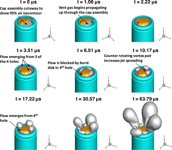
Figure 5. Instantaneous 3D flowfield visualized by iso-contours of 95% air mass fraction illustrating the propagation of vent gas and electrolyte vapor into the surrounding space during the initial venting (blowdown) process. Times shown are elapsed time from vent-activation.
Download figure:
Standard image High-resolution imageA closer inspection of the 95% air mass fraction iso-surface at t = 63.79 μs after initial venting (last frame of Fig. 5) is presented in Fig. 6. Figures 6a–6c show three different views of the 95% air iso-surface at t = 63.79 μs after initial venting. Inspection of the flowfield in Figs. 6a–6c revealed the presence of several secondary flows. Two counter-rotating vortex pairs (CRVP) and a corner vortex (CV) were identified. Figure 6a shows the 95% air iso-surface with a CRVP that entrains air on the top side of the jet (labeled as primary CRVP). Figure 6b shows another view of the primary CRVP as well as a secondary CRVP on the bottom side of the jet. Figure 6b also shows the formation of a CV. Figure 6c shows another view of the secondary CRVP and entrainment of fresh air at the bottom side of the jet.

Figure 6. Snapshot of flowfield at 63.79 μs after vent-activation showing iso-contours at 95% air mass fraction for three different views (a–c). In each view, three secondary flows are illustrated—primary CRVP, secondary CRVP, and CV. An x-normal section of 18650 cell model shows the location of a series of slices taken normal to the jet emerging from the cell (d). Zoomed-out, surface normal view of slice "f" showing Mach number contours (e). Contours of Mach number with in-plane flow streamlines (f–i) correspond to the planes shown in (d).
Download figure:
Standard image High-resolution imageFigure 6d shows a series of slices taken in the fluid region at t = 63.79 μs. The slices were taken at 45° relative to the horizontal, approximately normal to the jet emerging from the right side of the cell in Fig. 6d. Four slices labeled (f) through (i) move progressively farther away from the cell and correspond with the sub-figure labels in in Fig. 6. Figure 6e shows a zoomed-out view of Fig. 6f to help orient the position of the slices in sub-figures (f) through (i). Within each subfigure, contours of Mach number indicate the velocity magnitude normal to the plane, to visualize the primary flow pattern. The overlaid, in-plane streamlines indicate the secondary flow patterns.
Figure 6f shows the primary CRVP forming near the top of the vent hole. Moving away from the cell, Figs. 6g, 6h show the primary CRVP growing in size and entraining fresh air into the jet causing enhanced mixing with the vented gases. The enhanced mixing due to the presence of the primary CRVP was observed by the growth of the 95% air mass fraction iso-surfaces, shown most notably at t = 10.17 μs in Fig. 5 and in the corresponding video in the Electronic Supplementary Information. The CV propagated along the top of the cell casing, as shown in Fig. 6i, and enhanced mixing by spreading vent gases laterally along the top of the casing. The enhanced mixing due to the CV was observed at t = 63.79 μs in Fig. 5 and the corresponding video shown in the Electronic Supplementary Information. Figures 6g and 6h show the formation of the secondary CRVP. The secondary CRVP also contributed to enhanced mixing between the vent gas and surrounding fluid, but the effects were not as pronounced as the primary CRVP and CV when inspecting Fig. 5 and the corresponding video in the Electronic Supplementary Information.
Analysis of venting and cell state during non-VLE evaporation period
The venting flow and the internal state of the cell was compared at three different times to show the transition from the blowdown period to the non-VLE evaporation period: during blowdown (129.59 μs after vent-activation), transitioning from blowdown to non-VLE evaporation, (99.4 ms after vent activation), and during non-VLE evaporation (124.4 s after vent activation).
Figure 7 shows a z-normal slice of the computational domain where each row of images corresponds to a given flow time and each column corresponds to a particular field variable. For the three rows: Figs. 7a–7d corresponds to the instant at 129.59 μs after vent-activation, Figs. 7e–7h correspond to the instant at 99.4 ms after vent-activation, and Figs. 7i–7l correspond to the instant at 124.4 s after vent activation. For the four columns: contours of velocity magnitude are shown in Figs. 7a, 7e, 7i along with streamlines to visualize the flow pattern within the jellyroll, contours of mass fraction of gases are shown in Figs. 7b, 7f, 7j, contours of temperature are shown in Figs. 7c, 7g, 7k, and contours of the cathode reaction are shown in Figs. 7d, 7h, 7l. A video showing the z-normal slices of Fig. 7 is available in the Electronic Supplementary Material.

Figure 7. Instantaneous z-normal slices taken at three times following vent-activation showing velocity magnitude contours with streamlines visualization in the jellyroll (a), (e), (i), mass fraction of vented gases (b), (f), (j), temperature (c), (g), (k), and progress of cathode decomposition reaction (d), (h), (l). Images taken during blowdown at 129.59 μs after venting (a)–(d), during transition to non-VLE evaporation at 94.4 ms after venting (e)–(h), and during non-VLE evaporation at 124.4 s after venting (i)–(l).
Download figure:
Standard image High-resolution imageFigure 7a shows the maximum velocity magnitude in the jets emerging from the vent holes during blowdown exceeded 500 m s−1. At this instant in time, the internal pressure of the cell was 1.2 MPa above atmospheric pressure. The in-plane streamlines within the jellyroll show that the flow was aligned with the axis of the jellyroll and that the flow moved from the bottom of the cell upwards toward the vent cap.
Figure 7e shows that the jet velocity has decreased considerably at 99.4 ms after venting, from approximately 500 ms−1 in Fig. 7a to approximately 0.5 ms−1 in Fig. 7e. The reduced jet velocity corresponded to the reduction in pressure ratio across the vent cap since the internal cell pressure reached equilibrium with the surroundings within approximately 4 ms, as discussed previously in Fig. 3b. The jets no longer influenced the flow pattern around the cell. The average velocity within the cylindrical reactor was approximately 0.6 m s−1. As the flow passes the cell, it accelerates to maintain continuity, leading to a maximum velocity of approximately 0.8 m s−1 while the flow velocity through the vent holes was approximately 0.5 m s−1.
The in-plane streamlines within the jellyroll showed a bifurcation near the midline of the cell where flow either travels upward toward the vent or downward toward the space below the jellyroll. The bifurcated flow distribution within the jellyroll is consistent with previous, high-speed radiography. 32 Measurements by Finegan et al. showed globules of molten current collector travelling upwards to the headspace or downwards toward the space below the jellyroll, depending on the position within the jellyroll. 32 Electrolyte vapor was generated volumetrically within the jellyroll and the distributed mass traveled either downward or upward based on the path of least resistance. The open mandrel region in the center of the cell allowed gases to travel down the jellyroll and then back up the open mandrel region. The presence of a mandrel may increase the resistance to gases travelling up the mandrel region. For cells with a mandrel, flow may be forced entirely upwards through the jellyroll. In this respect, the present model may be useful in studying the conditions leading to jellyroll ejection. For the present work, the flow resistance upward and downward in the jellyroll were approximately equal and the bifurcation occurs at the midline of the cell. There were no significant differences in velocity magnitude and streamline patterns within the jellyroll when comparing 99.4 ms after venting, Fig. 7e, with 124.4 s after venting, Fig. 7i.
Contours of vented gas fraction (sum of electrolyte vapor and vent gas) in Figs. 7b, 7f, 7j support the conclusions drawn from inspection of the velocity contours. Figure 7b shows strong jet formation during blowdown at for 129.59 μs after vent-activation. The jets carry the vented gas away from the cell at an approximate 45° angle to the cell axis. As discussed in the previous section, mixing between the vented gas and surrounding air was enhanced by the RVs, CRVPs, and CVs. Figures 7f and 7j show that the plume of vented gases narrows as blowdown transitions to non-VLE evaporation period. The gases were entrained in the wake region above the cell and carried directly upward.
The temperature distribution within the cell and within the surrounding air space is shown in Fig. 7c for 129.59 μs after vent-activation and in Figs. 7g, 7k for 99.4 ms and 124.4 s after vent-activation, respectively. Figure 7c shows that the temperature distribution in the cell was approximately uniform at 180 °C during blowdown. The temperature of the gases emerging from the cell were substantially cooler as the rapid pressure decrease results in Joule-Thompson cooling. The amount of heat absorbed by the Joule-Thompson effect did not significantly influence the temperature of the cell, due to heat capacity of the jellyroll and other components which were two to three orders of magnitude larger than the heat capacity of the vent gas. The effect of evaporative cooling is clearly seen at 124.4 s, however, after vent-activation where the internal cell temperatures in Fig. 7k have decreased by ∼6 °C relative to Fig. 7c.
The progress of cathode reaction is shown in Fig. 7d for 129.59 μs after vent-activation and in Figs. 7h, 7l for 99.4 ms and 124.4 s after vent-activation, respectively. As discussed previously, evaporative cooling during the non-VLE period slowed, but did not stop, the cathode reaction. This was consistent with the increase in αc from a maximum of 0.30 in Fig. 7d to a maximum of 0.43 in Fig. 7l. At both time instants, the distribution of αc showed larger values toward the center of the cell. Increased temperature in the center of the cell led to local acceleration of decomposition reactions.
Analysis of venting and cell state during thermal runaway
Following the evaporative cooling period, the cell entered the Arrhenius heating period and progressed into thermal runaway. Figure 8 shows a z-normal slice of the computational domain, similar to Fig. 7. In the three rows of images: Figs. 8a–8d corresponds to a solution time of t = 49.9 min, Figs. 8e–8h correspond to t = 50.2 min, and Figs. 8i–8l correspond to t = 50.4 min. The solution times correspond to those shown Fig. 3b. The temperature rise rates were 95, 175, and 47 °C min−1 at t = 49.9, 50.2, and 50.4 min, respectively. For the four columns: contours of velocity magnitude are shown in Figs. 8a, 8e, 8i along with streamlines to visualize the flow pattern within the jellyroll, contours of vent gas mass fraction are shown in Figs. 8b, 8f, 8j, contours of temperature are shown in Figs. 8c, 8g, 8k, and contours of the electrolyte decomposition reaction are shown in Figs. 8d, 8h, 8l. A video showing the z-normal slices of Fig. 8 is available in the Electronic Supplementary Material.
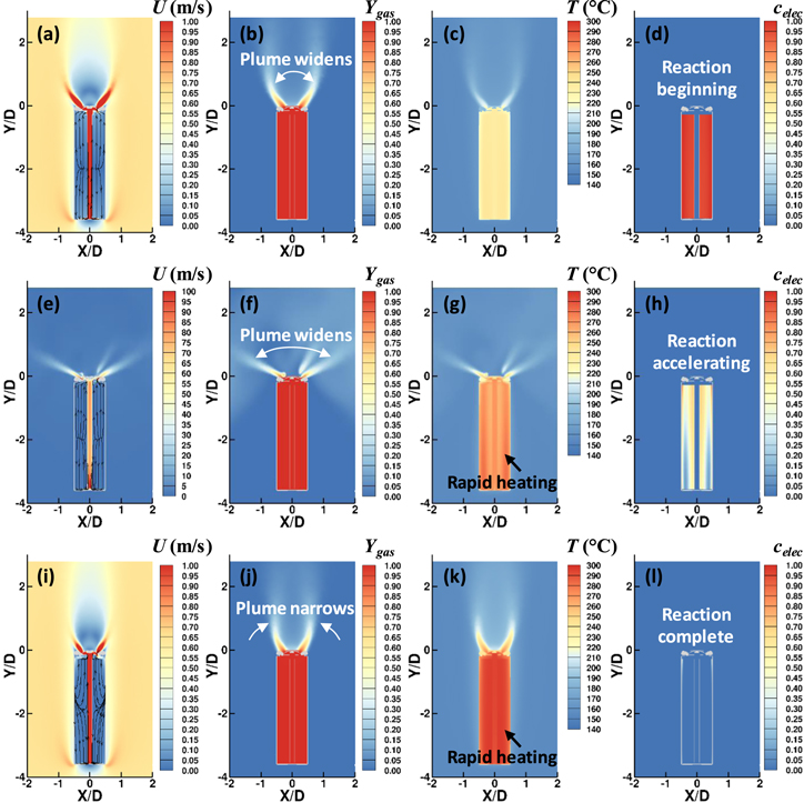
Figure 8. Instantaneous z-normal slices taken at three times during thermal runaway showing velocity magnitude contours with streamlines visualization in the jellyroll (a), (e), (i), mass fraction of vented gases (b), (f), (j), temperature (c), (g), (k), and progress of cathode decomposition reaction (d), (h), (l). Images taken at during thermal runaway at times of: 49.9 min (a)–(d), at 50.2 min (e)–(h), and 50.4 min (i)–(l).
Download figure:
Standard image High-resolution imageComparing Figs. 8a with 8e, the jet velocity increases by two orders of magnitude, from ∼1 ms−1 to ∼100 ms−1, as the cell enters thermal runaway from times t = 49.9 to 50.2 min, respectively. The increased jet velocity corresponded to increased gas generation, since the electrolyte decomposition reaction shows substantial progression between Figs. 8d and 8h. The electrolyte decomposition reaction slowed between t = 50.2 and 50.4 min, leading to a decrease in gas generation rate and a decrease in jet velocity when comparing Figs. 8e to 8i, respectively. Figure 8i shows that the jet velocity has decreased to a magnitude similar to that of Fig. 8a.
Contours of vent gas fraction show that the jets emerge at a shallower angle at t = 50.2 min, in Fig. 8f, when compared with t = 49.9 and 50.4 min, in Figs. 8b and 8d, respectively. The temperature distribution in Figs. 8c, 8g, 8k shows the progression into thermal runaway from Arrhenius heating. In Fig. 8c, the cell temperature approached 250 °C. In Fig. 8k the cell temperature approached 300 °C. The temperature of the vent gas plume also increased as the cell enters thermal runaway.
The electrolyte decomposition reaction progressed, almost to completion, between t = 49.9 min and 50.4 min. Figure 8d shows the electrolyte decomposition contour values are still near their initial value of celec = 1 at t = 49.9 min. Figure 8h shows that the reaction is accelerating as most of the cell shows celec < 0.5 at t = 50.2 min. Figure 8l shows that the electrolyte decomposition has progressed nearly to completion where most of the cell showed celec = 0, except for small regions near the top of the cell. The non-uniform distribution of the electrolyte decomposition reaction led to an evolving flow pattern within the jellyroll itself. Figure 8e shows that the bifurcation point, where flow either travels upward or downward, becomes shifted slightly downwards. The increased mass generation near the bottom of the cell caused an increase in flow resistance which resulted in more flow traveling upward. The same flow pattern was observed in the jellyroll in Fig. 8i.
The vent gas distribution into the surrounding space was compared, qualitatively, with experiments that captured images during initial venting (i.e. blowdown) and during thermal runaway and second venting. Garcia et al. 33 conducted experiments using Schlieren imaging to visualize the dispersion of electrolyte droplets emerging from the cell during initial venting. The authors also used natural luminosity imaging to visualize the flames emerging from the cell during thermal runaway and second venting. Figure 9 shows a comparison of simulations and experiments during these two events. Figure 9a shows the simulated mass fraction of vent gas during initial venting and Fig. 9b shows the distribution of electrolyte droplets imaged during initial venting in the experiments. The trajectory of the ejected material agrees, qualitatively, as visualized by the overlaid white lines on the simulation and experimental data. Similarly, Fig. 9d shows the simulated mass fraction of vent gas during thermal runaway and Fig. 9e shows the flame structure imaged during thermal runaway in the experiments. Overlaid white lines show the qualitative agreement between simulation and experiment when comparing the jet trajectory during thermal runaway and second venting. The simulations and experimental results both show that the vented material emerges at a steeper angle during blowdown and at a shallower angle during thermal runaway.

Figure 9. Qualitative comparisons between simulated jet trajectory of the present work with experiments conducted by Garcia et al. 33 (reproduced with permission from Elsevier): simulated mass fraction of vented gases during initial venting process (a), Schlieren image during initial venting (b), schematic of jet trajectory during initial venting (c), simulated mass fraction of vented gases during thermal runaway (d), and natural luminosity images taken during thermal runaway (e), and schematic of jet trajectory during thermal runaway (f). The jet trajectories (white solid lines in subfigures a,b,d,e) of simulations and experiments are qualitatively similar during the two stages of the thermal runaway process. The stagnation pressure from gases traveling up through mandrel space (f) causes jet trajectory to emerge at a shallower angle when compared to (c).
Download figure:
Standard image High-resolution image
The shallowing angle of the vent trajectory as the cell enters thermal runaway was discussed previously with Fig. 8 and is attributed to the differences of the pressure and velocity field within the cell during the two scenarios. During initial venting, the internal pressure is nearly 1.57 MPa and the gas mixture within the cell is stagnant. At the moment of vent-activation, the gases rush from the headspace and mandrel region, through the safety vent, and into the surrounding space as shown in Fig. 9c. In contrast, when the cell enters thermal runaway, a rapid generation of gas within the jellyroll results in an accumulation of gases in the mandrel space and gas travelling up the mandrel at high velocity (shown previously in Fig. 8e). The gases travelling up the mandrel create a stagnation pressure under the safety vent which alters the direction of vented gases emerging from the vents during second venting as shown in Fig. 9d. This observation is important for thermal propagation, where the jet angle may affect the heat transfer rates on nearby cells. Thus, accounting for the detailed flow physics within the cell and through the safety vent is necessary to accurately capture the jet trajectory with CFD-based thermal runaway models.
Conclusions
Thermal runaway of a small format, 18650 cell was analyzed using a 3D computational fluid dynamics framework to analyze the physics associated with venting, gas flow in the jellyroll, 3D reaction progression, and 3D cell heating. A highly detailed 3D geometric model allowed new insights into the physics of an oven test thermal abuse scenario. During initial venting blowdown process, shear force between the high momentum jet and the low momentum surrounding air led to the formation of a ring vortex (RV). Additional secondary flows identified during the blowdown process included: two counter rotating vortex pairs (CRVP) and a corner vortex (CV). The CRVPs were caused by shear forces between the high momentum jet and low momentum fluid near the walls of the vent. The CV was caused by the shear force between vent gases moving laterally along the positive terminal and the upward air draft around the cell. Of the four secondary flows identified, three contribute to the primary jets mixing with the surrounding fluid: RV, primary CRVP, and secondary CRVP. The fourth secondary flow, the CV, contributes to spreading the vent gases along the top of the cell casing. The secondary flows contribute to increased mixing between the vent gases and the surrounding air, as observed in the iso-surfaces of 95% air mass fraction. Increased mixing of vented hot gases with surrounding air may dilute the temperature of jets impinging on nearby surfaces, thus reducing the heat transfer rate.
After the initial blowdown, gas generation rate within the jellyroll influenced the jet velocity magnitude and vent gas plume. During the non-VLE evaporation period, jet velocity was reduced and the plume shape narrowed to the region directly above the cell. As the cell progressed into thermal runaway, the amount of mass generation increased due to the electrolyte decomposition reactions. As a result, jet velocity magnitude increased and the jets emerged at shallow angle, even more so than the angle of the initial jets during blowdown. After thermal runaway, decreased gas generation rate resulted in reduced jet velocity magnitude and a narrowed vent gas plume. The spatial distribution of vent gases plays a critical role in fire safety, as ignition of these gases will create a heat load on neighboring cells which is spatially dependent. In a module or pack, the orientation of the cells and the location of the failing cell may influence the rate of heat transfer from hot gases impinging on neighboring cells.
The present work provides the model framework needed to study the reacting flow scenario, where the vented gases ignite and create a heat load on neighboring cells. Ultimately, the spatial distribution of vented gases and the rate of mixing with surrounding air will play a key role in the predictive ability of thermal abuse models which include reacting flow and subsequent heat transfer in Li-ion modules and packs.
Acknowledgments
The authors acknowledge financial support from the Naval Surface Warfare Center, Crane Division under the Naval Innovative Science and Engineering Program. M. Parhizi acknowledges the Purdue Polytechnic Institute Post-Doctoral Fellowship Program for financial support on this project. W. Li acknowledges the Purdue University Andrews Fellowship Program and the Indiana Manufacturing Competitiveness Center (IN-MaC) for financial support on this project. The U.S. Government is authorized to reproduce and distribute reprints for governmental purposes notwithstanding any copy-right notation thereon. The views and conclusions contained herein are those of the authors and should not be interpreted as necessarily representing the official policies or endorsements, either expressed or implied, of the Naval Surface Warfare Center, Crane Division or the U.S. Government.
Supplementary data (1.6 MB PDF)
Supplementary data (0.2 MB PDF)
Supplementary data (0.7 MB MP4)
Supplementary data (0.4 MB MP4)
Supplementary data (1.7 MB MP4)