
Abstract
This article presents the development, parameterization, and experimental validation of a pseudo-three-dimensional (P3D) multiphysics aging model of a 500 mAh high-energy lithium-ion pouch cell with graphite negative electrode and lithium nickel manganese cobalt oxide (NMC) positive electrode. This model includes electrochemical reactions for solid electrolyte interphase (SEI) formation at the graphite negative electrode, lithium plating, and SEI formation on plated lithium. The thermodynamics of the aging reactions are modeled depending on temperature and ion concentration and the reactions kinetics are described with an Arrhenius-type rate law. Good agreement of model predictions with galvanostatic charge/discharge measurements and electrochemical impedance spectroscopy is observed over a wide range of operating conditions. The model allows to quantify capacity loss due to cycling near beginning-of-life as function of operating conditions and the visualization of aging colormaps as function of both temperature and C-rate (0.05 to 2 C charge and discharge, −20 °C to 60 °C). The model predictions are also qualitatively verified through voltage relaxation, cell expansion and cell cycling measurements. Based on this full model, six different aging indicators for determination of the limits of fast charging are derived from post-processing simulations of a reduced, pseudo-two-dimensional isothermal model without aging mechanisms. The most successful aging indicator, compared to results from the full model, is based on combined lithium plating and SEI kinetics calculated from battery states available in the reduced model. This methodology is applicable to standard pseudo-two-dimensional models available today both commercially and as open source.
Export citation and abstract BibTeX RIS

This is an open access article distributed under the terms of the Creative Commons Attribution 4.0 License (CC BY, http://creativecommons.org/licenses/by/4.0/), which permits unrestricted reuse of the work in any medium, provided the original work is properly cited.
List of Symbols
| Symbol | Unit | Meaning |
|---|---|---|
| Ae | m2 | Active electrode area |

| m2·m–3 | Volume-specific surface area of reaction n |

| F·m–3 | Volume-specific double-layer capacity |

| mol·m–3 | Concentration of species i in a bulk phase |

| mol·m–3 | Standard concentration of species i |
![${c}_{{{\rm{Li}}}^{+}[{\rm{elyt}}]}$](https://content.cld.iop.org/journals/1945-7111/170/2/020525/revision2/jesacb8e1ieqn5.gif)
| mol·m–3 | Concentration of solved Li-ions |

| J·kg–1·K–1 | Specific heat capacity |

| m2·s–1 | Diffusion coefficient of species i |

| m2·s–1 | Effective diffusion coefficient of species i |

| J·mol–1 | Activation energy of forward reaction |

| C·mol–1 | Faraday's constant |

| J·mol–1 | Enthalpy of reaction n |

| kJ·mol–1 | Molar enthalpy of species i |

| J·mol–1 | Gibbs energy of reaction n |

| 1 | Index of species |

| A·m–2 | Area-specific current (with respect to  ) ) |

| A·m–2 | Exchange current density |

| A·m–2 | Exchange current density factor |

| A·m–3 | Volume-specific faradaic current |

| 1 | Index of bulk phases |

| W·m–2 | Heat flux from cell surface |

| mol·m–2·s–1 | Molar flux of species i |

| mol, m, s (*) | Forward and reverse reaction rate constants |

| m | Thickness of electrode pair |

| kg·mol–1 | Molar mass of species i |

| 1 | Index of reactions |

| 1 | Number of reactants and products in reaction |

| 1 | Number of reactions |

| Pa | Pressure |

| Pa | Reference pressure |

| W·m–2 | Heat source due to chemical reactions |

| W·m–2 | Heat source due to ohmic losses |

| W·m–3 | Volume-specific heat source |

| J·K–1·mol–1 | Ideal gas constant |

| Ω·m2 | Area-specific ohmic resistance of current collection system |

| Ω·m3 | Volume-specific ohmic resistance of SEI film |

| mol·m–2·s−1 | Interfacial reaction rate of reaction n |

| J·mol–1·K–1 | Molar entropy of species i |

| mol·m–3·s–1 | Volumetric species source term |

| mol·m–3·s–1 | Volumetric species source term due to double layer charge/discharge |

| s | Time |

| K | Temperature |

| K | Ambient temperature (cell surrounding) |

| m3 | Volume of cell |

| m | Spatial position in dimension of battery thickness |

| 1 | Stoichiometry of lithium in the AM |

| 1 | Mole fraction |

| m | Spatial position in dimension of electrode-pair thickness |

| m | Spatial position in dimension of particle thickness |

| 1 | Number of electrons transferred in charge-transfer reaction |

| W·m–2·K–1 | Heat transfer coefficient |


| 1 | Anodic and cathodic transfer coefficients of electrochemical reaction |

| V | Electric potential in the solid phase and in the electrolyte |

| V | Equilibrium potential difference |

| V | Electric potential of the negative electrode |

| V | Equilibrium potential of plating reaction |

| V | Electric potential difference of reaction n |

| 1 | Emissivity of the cell surface |

| 1 | Volume fraction of phase j |

| V | Activation overpotential |

| W·m–1·K–1 | Thermal conductivity |

| J·mol–1 | Standard-state chemical potentials of all species i |

| 1 | Stoichiometric coefficient of species i |

| 1 | Stoichiometric coefficient of electrochemical reaction n |

| kg·m–3 | Density |

| W·m–2·K–4 | Stefan-Boltzmann constant |

| 1 | Geometric tortuosity of the electrolyte |

| 1 | Simulated aging indicator |

| m3·mol–1 | Partial molar volume of species i |
| * Units of mol, m and s depending on reaction stoichiometry | ||
Lithium-ion batteries play a vital role in a society more and more affected by the impact of climate change. They appear as the ideal candidates for climate-neutral technologies such as electric mobility and renewable energy storage. 1,2 However, further research and development is required to understand their behavior, predict their issues and therefore improve their performance. The macroscopically observable behavior of lithium-ion cells in terms of current, voltage, temperature and aging dynamics is governed by a strong coupling of electrochemistry and transport on multiple scales inside the cell. Mathematical modeling and numerical simulation have proven to be highly useful 3 to unravel the impact of the multi-scale and multi-physical internal processes on macroscopic cell behavior, thus increasing the predictivity of life expectancy models. Nevertheless, the explanatory power of simulations is only significant if the model is thoroughly validated experimentally.
The lifetime of a battery is affected by various aging mechanisms happening at the electrode scale and causing capacity and power fade over time. 4–7 Macroscopically, two types of aging drivers are distinguished: calendaric aging, during storage and in case of nonoperating conditions, and cyclic aging, during charging/discharging operations. 8 In this study we will focus mainly on cyclic aging. Microscopically, aging results from chemical reactions driven by concentration, potential and/or temperature as well as structural and morphological changes inside the electrodes. This leads to specific degradation modes, referred to as loss of lithium inventory (LLI) and loss of active material (LAM). 9,10 In this study we apply a microscopic, physically-based approach towards aging.
The first chemical aging mechanism 11 here included, considered as the most common source of capacity fade, is the loss of lithium inventory 9,12–15 to the solid electrolyte interphase (SEI) at the negative electrode (NE), the formation of which competes with reversible lithium intercalation. As the graphite electrodes of lithium-ion cells operate at voltages beyond the thermodynamic stability of the organic electrolytes, the electrochemical reduction of the electrolyte solvent and decomposition of the conducting salt are inevitable, with the resulting products forming a passivating film at the graphite/electrolyte interface which is permeable for lithium ions, but rather impermeable for electrons and other electrolyte components. 7,16 Over time SEI growth and thickening leads to LLI and capacity loss. 17 The continuous volume changes of the graphite particles during cycling strongly stress the limitedly flexible SEI layer, 18,19 hence a repetitive fracture of the already formed nanometer-thick film could happen, with a further exposition of the underlying surfaces. 20 We include this mechanism using an SEI formation rate law depending on SOC-dependent stress on the SEI. 8
The second chemical aging mechanism 21 included in our modeling framework is lithium plating. During charging at high currents and/or low temperatures, a high overpotential is reached at the graphite NE and hence a dropping of the NE potential below 0 V vs Li/Li+. 22–25 Under these conditions, lithium plating may become favorable over the main reaction of intercalation into the graphite particles. Macroscopically, lithium plating can be identified by specific "plating hints" in the voltage behavior: the most known is a specific plateau in the cell voltage, observed during relaxation or discharge after charge at low temperatures 26–36 and ascribed to the mixed potential associated with simultaneous oxidation of deposited lithium and intercalated lithium.
Lithium plating is generally reversible (the metallic lithium formed during charging becomes dissolved or re-intercalates during rest or subsequent discharge 21 ). However, the high reactivity of metallic lithium towards the organic electrolyte leads to immediate follow-up reactions, in particular, the additional formation of SEI. This is the main cause for LLI and associated capacity loss due to plating. 5,11,37,38 The multiple causes, rates and inter-dependencies of these aging mechanisms make a complete analysis of the aging phenomena extremely challenging.
This article introduces a new approach to the highly topical issue of fast charging in batteries, as shown in Fig. 1. The first part of the study focuses on the development, parameterization, and experimental validation of a pseudo-three-dimensional (P3D) aging model of a commercial 500 mAh high-energy lithium-ion pouch cell with graphite NE and lithium nickel manganese cobalt oxide (NMC) positive electrode (PE). The P3D model 39,40 features transport on three 1D scales; apart from lithium transport in the particles (microscale) and mass and charge transport along the electrode pair (mesoscale), it includes a thermal model along the cell thickness (macroscale) that allows to predict temperature gradients both in time (during cycling) and space (along the cell thickness). Into this model, we integrate electrochemical reactions for SEI formation on graphite, lithium plating, and SEI formation on plated lithium. The combined model is hereafter referred to as "full model" (FM), which is able to describe cell aging over a wide temperature range. This first part introduces the following original features: (i) systematic parameterization of thermoelectrochemistry and P3D transport using combined literature and original experimental data, both in the time and frequency domains; (ii) experimental aging using charging rates beyond the manufacturer's recommendation, thus inducing accelerated aging, in order to avoid long-term measurements; (iii) identification of critical operation conditions by model-based quantification of capacity loss due to cycling and visualization of aging colormaps as function of both temperature and C-rate.

Figure 1. Present approach towards the limits of fast charging in batteries. It is possible to simulate the operating limits using aging indicators calculated from the output of standard pseudo-2D "Newman-type" models without aging mechanisms.
Download figure:
Standard image High-resolution imageThe second part of the study aims to transfer these results to "Newman-type" pseudo-two-dimensional (P2D) models 41,42 used today as standard tools, for example, in industrial applications. This type of model is hereafter referred to as "simple model" (SM). This model does not include the thermal scale (hence, all simulations are isothermal) and does not include aging reactions. Instead, we derive aging indicators that can be calculated by post-processing simulations from a P2D model. This avoids the effort in time and cost for developing and parameterizing the sophisticated aging model presented in the first part. Two originals features are here introduced: (iv) development of different aging indicators derived from a P2D model without aging mechanisms; (v) evaluation of the indicator approach by comparison with our reference P3D, using a specifically developed "Goodness of Indicator" (GoI) factor.
Modeling and Simulation Methodology
This section gives an overview of the P3D modeling and simulation approach. Details are presented in the Appendix of this paper. The study is devoted to a commercial 3.7 V 500 mAh high-energy lithium-ion pouch with graphite at the NE and NMC at the PE. Details on the cell is given below in the experimental section.
Pseudo-3D transport
We use a P3D model that was originally developed for studying aging in high-power lithium iron phosphate/graphite cylindrical cells. 40 We reparameterized it for representing high-power lithium-ion pouch cell with graphite at the NE and NCA/LCO blend at the PE. 39,43 Here, lithium plating was added. 11,21 These studies demonstrate the versatility of P3D models with detailed chemistry. The transport scales are shown schematically in Fig. 2 and combine heat transport through the cell thickness and holder plates (in this paper referred to as macroscale or x scale), mass and charge transport inside the liquid electrolyte (mesoscale, y scale), and diffusive mass transport in the active materials (AM) particles (microscale, z scale), each solved in 1D and coupled via appropriate boundary conditions and upscaling relationships. Heat transport is described via conduction and uses heat source terms due to chemical reactions and ohmic losses. The electrodes are described in a continuum setting, that is, microstructure is not resolved. Transport of electrolyte-dissolved ionic species (Li+ and PF6 –) is described as combined diffusion and migration in a Nernst-Planck setting with concentration-dependent diffusion coefficients. The lithium transport in the AM is modeled by Fickian diffusion with stoichiometry-dependent diffusion coefficient. The chemistry is described within a generalized framework allowing an arbitrary number and type of reactions at each of the involved interfaces. Thermodynamics and kinetics are evaluated with the open-source software Cantera, 44 allowing a consistent definition and simple exchange of parameters. For details please see the Appendix and our previous works. 11,21,39,40

Figure 2. Schematic representation of 1D+1D+1D (pseudo-3D, P3D) modeling domain with macroscale (x), mesoscale (y) and microscale (z).
Download figure:
Standard image High-resolution imageIn the present work, we completely re-parameterized the model in order to represent the target cell and its aging behavior, then we validate the model by comparing simulations with experiments over a wide range of conditions.
In the present P3D model, the cell is represented by one single electrode pair on the macroscale. This means that only one single electrode-pair model (P2D model on the two lower scales) is used to describe electrical cell performance. The heat production calculated from the electrode pair is upscaled and evenly distributed over the macroscale. Spatial temperature gradients result from conduction along the cell thickness and convective heat losses at the surface. The average temperature on the macroscale is passed back to the P2D model. While predicted average temperature increase during cycling is notable (up to 1 °C at 2 C), predicted spatial temperature gradients are only small (<0.1 °C) for the thin (3.2 mm) pouch cell investigated here, thus justifying the use of only one electrode pair. The present modeling framework can also be applied to larger cells, where temporal and spatial temperature gradients can be considerably larger.
Electrochemistry
In the present model, the electrochemical reactions include two intercalation/de-intercalation charge-transfer reactions (NMC and graphite), the reversible plating and the two SEI formation reactions (with Li+ ions and Li metal as reactants, respectively). Required model parameters are rate coefficients and activation energies of all reactions as well as the double-layer capacitances of the two electrodes.
The reaction mechanism and rate coefficients are given in Table I. Intercalation/de-intercalation parameters (cf. Table I, Reactions 1, 5) were determined by fitting simulated EIS data to experimental values for individual temperatures, while activation energies were determined from Arrhenius plots (see Appendix). For the reversible plating reaction (cf. Table I, Reaction 2), we adopted the plating kinetics from our previous work
21
which had previously been derived by Ecker.
35
The model includes SEI formation via two different pathways
11
: one is "electrolyte-driven" (cf. Table I, Reaction 3) and forms SEI via the reaction of Li+ ions and electrons with the electrolyte. The rate expression includes accelerated kinetics from SEI cracking due to volume changes of the graphite particles during cycling
8,19
. The other pathway, "plating-driven" (cf. Table I, Reaction 4), operates via a direct reaction of plated metallic lithium with electrolyte without charge transfer. Microscopically, this reaction takes place on the surface of plated lithium. In order to describe the positive feedback between plating and SEI formation, we set the plating-driven SEI formation rate proportional to the lithium volume fraction, that is,  ∼
∼ The SEI itself is assumed as ideally uniform in morphology and chemical composition, consisting of only lithium ethylene dicarbonate (LEDC), (CH2OCO2Li)
Table I. Interfacial chemical reactions and rate coefficients ("elyt-driven" = electrolyte-driven, "LP-driven" = lithium plating-driven).
| No. | Electrode | Reaction | Label | Rate coefficient | Activation energy | Symmetry factor |
|---|---|---|---|---|---|---|
| (1) | Negative | Li+[elyt] + e– + V[C6] ⇄ Li[C6] | Intercalation |
 = 1.86·1013 A m−2 = 1.86·1013 A m−2
| 75.4 kJ mol−1. 39 | 0.5 |
| (2) | Negative | Li+[elyt] + e– ⇄ Li[metal] | Plating |
 = 2.29·1013 A m−221,35 = 2.29·1013 A m−221,35
| 65.0 kJ mol−1. 35 | 0.492. 35 |
| (3) | Negative | Li+[elyt] + C3H4O3[elyt] + e– ⇄ 0.5 LEDC[SEI] + 0.5 C2H4 | SEI formation (elyt-driven) |
 = = ![$\left(\displaystyle \frac{1}{{{\boldsymbol{\delta }}}_{{\bf{S}}{\bf{E}}{\bf{I}}}}+{{\boldsymbol{k}}}_{{\bf{c}}}\cdot {{\boldsymbol{i}}}_{{\bf{c}}{\bf{h}}{\bf{g}}}^{{\boldsymbol{V}}}\cdot \displaystyle \frac{{\bf{d}}{{\boldsymbol{\sigma }}}_{{\bf{t}},{\bf{S}}{\bf{E}}{\bf{I}}}}{{\bf{d}}{{\boldsymbol{X}}}_{{\bf{L}}{\bf{i}}\left[{{\bf{C}}}_{6}\right]}}\right)\cdot 8.65\cdot {10}^{-11}$](https://content.cld.iop.org/journals/1945-7111/170/2/020525/revision2/jesacb8e1ieqn79.gif) mol/(m2·s).
8
,
a) mol/(m2·s).
8
,
a)
| 55.5 kJ mol−1. 8 | 0.5 8 |
| (4) | Negative | Li[metal] + C3H4O3[elyt] ⇄ 0.5 LEDC[SEI] + 0.5 C2H4 | SEI formation (LP-driven) |
 = =  4.65·10-7 mol/(m2·s)
b) 4.65·10-7 mol/(m2·s)
b)
| 5.0 kJ mol−1. b) | 0.492 35 |
| (5) | Positive | Li+[elyt] + e– + V[NMC] ⇄ Li[NMC] | Intercalation |
 = 1.17 ·1011 A m−2 = 1.17 ·1011 A m−2
| 61.4 kJ mol−1. 39 | 0.5 |
a)Reaction rate set to represent both calendaric and cyclic SEI formation, see Ref.8,11. b)Reaction rate set proportional to plated lithium volume fraction  Values fitted to simulate experimental aging data.
All charge-transfer reactions are modeled with Butler-Volmer kinetics, while plating-driven SEI formation is a thermochemical reaction where the rate is described by standard mass-action kinetics (cf. Appendix). The kinetic parameters are area-specific, and we assume the reaction surface area to be constant and independent of lithium volume fraction. Hence, the present model does not consider effects like blocking of the graphite surface by metallic lithium or detachment of metallic lithium fragments.
Simulation methodology
The P3D model presented above is implemented in the in-house multiphysics software package DENIS (Detailed Electrochemistry and Numerical Impedance Simulation) 40 and numerically solved using the implicit time-adaptive solver LIMEX. 45,46 The spatial derivatives were discretized in a finite-volume scheme, using 20, 19 and 11 non-equidistant control volumes on the x, y and z scales, respectively.
The chemical thermodynamics and kinetics are evaluated with the open-source code Cantera 44 (version 2.5.0a3), which is coupled to the DENIS transport models via the chemistry source terms. An in-depth explanation about modeling lithium-ion batteries with Cantera can be found in Mayur et al., 47 further details are given in the Appendix.
MATLAB (version 2019a) is the interface for controlling all DENIS simulations, as well as for data evaluation and visualization. Electrochemical impedance simulations were performed using a current step/voltage relaxation protocol and subsequent Fourier transform. 48
Experimental Methodology
This section presents the cell-level and electrode-level experiments that were carried out in order to obtain parameters and validation data required for modeling.
Investigated cells
All experiments used 3.7 V 500 mAh high-energy lithium-ion pouch cells by the manufacturer Hunan CTS Technology Co., Ltd, China, cell model 333450. A total of 200 cells were purchased and 19 individual cells from the same batch were used for this study. The cell chemistry is graphite at the NE and NMC at the PE. The manufacturer specifies upper and lower cut-off voltages of 4.2 V and 3.0 V.
Geometrical and morphological analyses
A pouch cell in pristine state was discharged down to the lower voltage limit of 3.0 V with a constant current of 0.012 C, then disassembled in an Argon-filled glove box under a monitored atmosphere with a water and oxygen content of less than 0.1 ppm. The electrodes and separator were rinsed with dimethyl carbonate (DMC) to remove all electrolyte residues. The total active electrode area was measured with a ruler, and the thicknesses of NE, PE, separator, and current collector were measured with a digital micrometer. Additionally, the mean particle size of both electrodes was determined optically with a Keyence Light Microscope VHX-7000. The measured values of the aforementioned parameters are listed in Table VI.
Half-cell measurements
Half-cells measurements were carried out using PAT-Cell test cells from the company EL Cell, Germany. Harvested electrode rolls from the disassembled pouch cell were used for the assembly of experimental half-cells. Since the electrode rolls are coated with AM on both sides, we used N-Methyl-2-pyrrolidone (NMP) to remove the coating from one side. Next, the electrodes were punched into circular disks with 18 mm diameter, followed by a rinsing step in dimethyl carbonate (DMC) to remove any impurity. Pure lithium metal disks with the same diameter of 18 mm were prepared as counter electrodes. Apart from the electrodes, the test cell setup includes a PAT-Core, which comprises of a polypropylene insulation sleeve, a 220 μm thick polypropylene (PP) fibre/polyethylene (PE) membrane separator, a reed contact and a lithium metal reference ring. For electrolyte, we used 103 μl of 1 M LiPF6 in EC:DMC 1:1 (v:v).
After the assembling of the experimental cells, a formation process was carried out with two constant current (CC with 4.4 mA) cycles and a third constant current-constant voltage (CC–CV) cycle. PE half-cells were cycled between 3.0 V and 4.3 V, whereas the voltage range for NE half-cells was 0.05 V to 0.8 V. After the cell formation, the OCV curves were obtained by applying a constant current of 0.088 mA in both charging and discharging directions. Both formation and OCV measurement were conducted using a battery cycler BaSyTec CTS LAB XL and inside a Friocell 55 climate chamber at 20 °C.
Electrochemical measurements of full cells
Electrochemical investigations of full cells were carried out with a battery cycler (BaSyTec CTS Lab XL) combined with an impedance analyzer (Zahner IM6 Electrochemical Workstation) in a climate chamber (MMM Group Fricocell 55). The investigated cell was placed between two aluminum plates, each with a thickness of 10 mm, to ensure symmetrical convection condition as the cell heats up under load. Due to the good thermal conductivity of aluminum, heat generated in the cell can be transferred to the surrounding air. Surface temperature of the cell was measured using an NTC sensor, which is embedded in the center of the base aluminum plate.
Electrochemical impedance spectroscopy (EIS) measurements were performed at different SOCs (20%, 35%, 50%, 65%, 80%, 100%) and at different temperatures (5 °C, 20 °C, 35 °C, 50 °C). The EIS measurements were recorded in galvanostatic mode by applying an excitation current of 20 mA within the frequency range of 10−2 Hz to 105 Hz. Before carrying out the EIS measurements, a discharge curve of the cell was obtained by discharging the cell with a small current of 50 mA (0.1 C) from a fully charged state at 20 °C (Step I). Based on the discharge curve, the quasi-open circuit voltages at the respective SOCs were obtained (Step II), with these values served as the cut-off voltages for the SOC adjustment in Step IV. For the first EIS measurement at 20 °C, the cell was charged to 100% SOC using a CCCV protocol (0.1 C, with cut-off current C/20), followed by a 1 h rest period (Step III). After the completion of the EIS measurement at 100% SOC, SOC adjustment (100% SOC to 80% SOC) was carried out by discharging the cell with a CCCV protocol (0.1 C, with cut-off current C/20), followed by a rest period of 1 h before carrying out the EIS measurement (Step IV). This SOC adjustment protocol was applied to the subsequent measurements, i.e. at 65%, 50%, 35% and 20% SOC (Step V). After the completion of the last EIS measurement at 20% SOC and 20 °C, the temperature was increased to 35 °C (Step VI). Step I to Step VI were repeated for the EIS measurements at 35 °C, 50 °C and 5 °C. At 5 °C, rest period of 1 h was insufficient for the cell to achieve a steady-state OCV after the adjustment to 100% SOC, thus, a total rest period of 5 h was applied.
Three different types of time-domain experiments were carried out in order to characterize the electrochemical and aging behavior, subsequently denoted as protocols A, B and C. In protocol A, the characteristics of the cell under non-aging conditions were investigated at different temperatures (5 °C, 20 °C, 35 °C, 50 °C) and at varying discharge current (0.05 C, 0.5 C, 1 C, 2 C, 3 C). The measurements were carried out by following a CCCV protocol in both charging and discharging directions with CV cut-off current C/20. To prevent possible aging effects caused by lithium plating, the charging current for every cycle was kept at a low current (0.2 C, with cut-off current C/20). For the same reason, we cycled the cells in such order: 20 °C, 35 °C, 50 °C, 5 °C, keeping measurements at 5 °C to the last, since a cell cycled at low temperature is more susceptible to lithium plating. Starting from a fully-discharged cell, successive cycles were performed for each temperature, with a rest period of 10 h allowed during the temperature change.
To investigate the cell behavior in the presence of aging, we carried two additional experiments. In protocol B, charge-discharge cycles were recorded at different temperatures (20 °C, 35 °C, 50 °C, 5 °C) and various C-rates (0.5 C, 1 C, 2 C, 5 C) in both charging and discharging directions. By applying charging currents greater than 1 C (thereby exceeding the manufacturer's recommended maximum charging current of 1 C), we induced aging due to lithium plating. Additionally, to capture the electrochemical behavior caused by calendar aging, we performed the same charge-discharge protocol at 20 °C with C-rates of 0.5 C, 1 C, 2 C, 5 C after a total storage time of 5 months at 20 °C.
Finally, for protocol C, cycles with discharge at a fixed C-rate (1 C) and varying charge rates were performed at 20 °C. Starting from a fully-discharged cell, successive cycles were performed with the following protocol: various CC charge (0.05 C, 0.5 C, 1 C, 2 C, 4 C) and fixed 1 C CCCV discharge, with cut-off current C/20.
Detection of lithium plating
Voltage relaxation 33 and cell expansion 49 were introduced as methods for detecting lithium plating. Both cell cycling and data acquisition of cell thickness were carried out with a BaSyTec CTS Lab XL to validate the simulation results.
The voltage relaxation measurement was performed on two cells, respectively at 5 °C and 20 °C, by charging with CC (0.5 C, 1 C and 2 C) from a discharged state to the upper voltage limit of 4.2 V, then followed by a 2 h rest period to monitor the voltage relaxation of the cells. At 20 °C, an evident voltage plateau was observed in the relaxation curve following 2 C CC charge, indicating the presence of plating from the charging step. For the measurements at 5 °C, no voltage plateau was detected at any of the charging rates.
A short cycling test was carried out at 5 °C on a third cell with a variation of charging current amplitudes (0.5 C, 1 C and 2 C) in sequence. For each charging C-rate, the cell was cycled for five times, following a CCCV charge—2 h rest—1 C CCCV discharge—2 h rest protocol. C/20 CV cut-off was used for (dis)charging. Irreversible cell expansion was observed at all three charging currents of 0.5 C (0.143 mm), 1 C (0.147 mm) and 2 C (0.213 mm).
An additional long cyclic aging test was performed as follows. Two cells were cycled at 20 °C for a total of 100 cycles, following a CCCV charge–30 min rest—CCCV discharge—30 min rest protocol. Apart from the charging current (1 C and 2 C, respectively), both cells had the same discharging current of 1 C and cut-off current of C/20. Minor capacity fade and smaller increase in cell thickness was detected at 1 C, with the capacity decreasing by 0.71% after 50 cycles and a total of 2.80% after 100 cycles. On the other hand, the cell charged at 2 C already experienced a capacity fade of 5.8% after only 5 cycles, with the decrease in capacity continued steadily to 13.47% after 100 cycles. The cell thickness was also measured at the end of 100 cycles, with the cells charged at 1 C and 2 C showing an increase by 0.09 mm and 0.17 mm, respectively.
Results of "Full Model" and Experiments
In this section, the macroscopic electrochemical behavior of the cell in the time domain is shown over a wide range of conditions. A systematic comparison between simulations and experiments is carried out and discussed. All simulations were performed with the FM using a single set of parameters.
Time-domain electrochemical behavior in absence of aging
In Fig. 3 simulated CCCV discharge curves are compared with experimental data at different temperatures and C-rates. Simulations were performed at different temperatures (20 °C, 35 °C, 50 °C, 5 °C) with protocol A described in "Electrochemical measurements of full cells" (CCCV charge at a fixed low C-rate of 0.2 C followed by variable CCCV discharge at 0.05 C, 0.5 C, 1 C, 2 C and 3 C, with cut-off current C/20). The CCCV charge and the rest period of 10 h are not shown in Fig. 3. The results of our simulations show a qualitatively good agreement with experiments. The model fidelity is generally better at lower C-rates compared to higher C-rates. In particular, the broadening and loss of features in the discharge curves as well as the increasing asymmetry between charge and discharge curves 50 observed experimentally with increasing C-rate is not well reproduced by the model. It is noteworthy that our model reproduces very well the decrease in charge capacity at 5 °C (max charge throughput at 506 mAh at 0.05 C in Fig. 3d), but it is not able to reproduce the small increase observed at 35 °C and 50 °C (531 and 535 mAh at 0.05 C, respectively Figs. 3b and 3c).
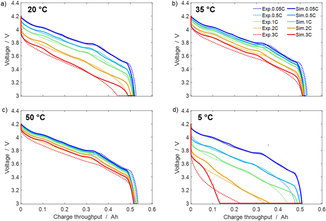
Figure 3. Experimental and simulated CCCV discharge cycles at (a) 20 °C, (b) 35 °C, (c) 50 °C, (d) 5 °C. Protocol: fixed 0.2 C CCCV charge, with cut-off C/20 (not shown here) - CC discharge (0.05 C, 0.5 C, 1 C, 2 C, 3 C) - CV discharge (cut-off C/20). A rest period of 10 h is allowed during temperature change.
Download figure:
Standard image High-resolution imageTime-domain electrochemical behavior in presence of aging
In Fig. 4 simulated CCCV charge-discharge cycles for protocol B (cf. "Electrochemical measurements of full cells") are compared with experimental data at different temperatures and various C-rates for both discharging and charging (0.5 C, 1 C, 2 C, 5 C). Starting from a fully discharged cell, successive cycles are performed for each temperature: 20 °C (a), 35 °C (b), 50 °C (c), 5°C (d) and then 20°C again (e), after a simulated break to replicate the experimental 5 months storage time (see "Electrochemical measurements of full cells"). Both simulations and experiments were carried out according to the following protocol: CCCV charging (cut-off current C/20) - CCCV discharging (cut-off current C/20), with a rest period of 10 h only allowed during the temperature change.

Figure 4. Experimental and simulated CCCV charge/discharge cycles at (a) 20 °C, (b) 35 °C, (c) 50 °C, (d) 5 °C, (e) 20 °C after storage. Protocol: CCCV charge - CCCV discharge (0.5 C, 1 C, 2 C, 5 C, with cut-off C/20). A rest period of 10 h is allowed during temperature change. In this representation, the lower branches represent discharge (time progressing from left to right) while the upper branches represent charge (time progressing from right to left). Both, charge and discharge curves, are assigned a charge throughput (x axis) of zero for a fully-charged cell (i.e., after CCCV charge).
Download figure:
Standard image High-resolution imageFigure 4 shows severe aging during cycling with an evident decrease in charge capacity at C-rates > 1 C as early as 20 °C (Panel a): it can be concluded that the cell is strongly susceptible to plating and SEI formation. In Panels b) and c), respectively 35 °C and 50 °C, the charge capacity does not decrease with cycling but at 5 °C (Panel d) we observe quite a capacity drop, with the charge capacity at 2 C being as low as ∼380 mAh (at 5 C simulations underpredict the decrease observed experimentally - 370 mAh vs 336 mAh). It is possible to deduce the presence of plating by observing some peculiarities in the simulated discharge cycles at 5 C 20°C (Panel a) and for all C-rates at 5°C (Panel d): these "bumps" below 0.1 Ah correspond to voltage plateaus, due to the oxidation and eventual re-intercalation of the plated lithium formed during CCCV charging 26–36 . In Fig. 4e we observe an increase again in the charge capacity, which is likely a matter of cycling at higher temperature (20°C for the aged cell vs the previous at 5 °C). Simulations here overpredict the capacity increase observed experimentally (for all C-rates, ∼390 mAh vs ∼360 mAh). To sum up the discussion of Fig. 4, the results of our simulations show generally a good agreement with the experiments for the wide range of C-rates and temperatures applied here.
The physicochemical model allows an insight into internal battery states. As the present model includes a continuity equation for both SEI and metallic lithium, 21 we can access the volume fractions during cycling. The data series shown in Fig. 4 is resumed in Fig. 5 by plotting selected observables and internal states over the C-rates for all temperatures. Each data point represents a single cycle, with overall experimental time progressing from left to right (i.e., the experiments started at 20 °C and 0.5 C, continued with 20 °C and 1 C, etc.). Panel (a) (simulations and experiments compared) shows the charge capacity for each individual charge. These data illustrate nicely how certain experimental conditions (in particular, low temperatures and high C-rates) lead to a decrease of capacity which irreversibly progresses into the following cycle. The data also illustrate the capability of the model to reproduce the experimental observations, that is, the model ages in a similar way than the experiments.
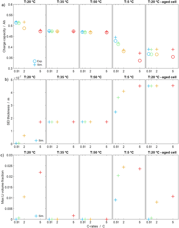
Figure 5. Based on the data of Fig. 4, in (a) charge capacity (both simulations and experiments), (b) SEI thickness (simulations only) as well as (c) maximum lithium volume fraction during charge (simulations only). All data points from left to right represent progressing experimental time: the experimental cycles started at 20 °C and 0.5 C (first cycle, first data point in the plots), continued with 20 °C and 1 C (second cycle, second data point in the plots), etc., consecutively going over all C-rates (0.5 C, 1 C, 2 C, 5 C) and repeating the cycles at different temperatures (20 °C, 35 °C, 50 °C, 5 °C, 20 °C after storage).
Download figure:
Standard image High-resolution imagePanel (b) and Panel (c) of Fig. 5 (both simulations only) show respectively the increasing SEI thickness and the maximum plated lithium volume fraction during each cycle. Panel (b) displays how the SEI layer thickens during cycling at 20 °C and, even more so, at 5 °C; at 35 °C, 50 °C and 20 °C (aged) no increase happens, consequently we can explain the capacity fade in Figs. 4a, 4d with the lithium-consuming SEI formation. On the other hand, plating in Panel (c) does not follow a constant trend but, being reversible, is caused by a combination of thermodynamics and kinetics according to cycling temperature. The highest plated lithium volume fraction is predicted at 5 °C and high C-rates, while at 50 °C, no plating occurs at all. As the plating-induced SEI formation rate is assumed proportional to the lithium volume fraction, large lithium volume fractions cause a fast increase of SEI thickness. It is interesting to note that the two 20 °C data sets show a different experimental behavior. Capacity loss after 2 C and 5 C rates is observed only for the initial data set, but not for the final one. The simulations are able to reproduce this finding.
According to protocol C (cf. "Electrochemical measurements of full cells"), experiments and simulations of consecutive cycles with varying CC charge rate (0.05, 0.5 C, 1 C, 2 C, 4 C) and CCCV discharge at a fixed C-rate (1 C, cut-off current C/20) were performed at 20 °C. In Fig. 6 the results are compared with the experiments (cf. "Experimental Methodology"). The charge throughput values of the curves in Fig. 6 are normalized at the end of CC charge (i.e., all cycles begin at 0 Ah to better show the progressive capacity loss due to fast charging). The results of our simulations show generally good agreement with the experiments, in particular including at 2 C and 4 C: the specific appearance below 0.1 Ah of the discharge curves at higher C-rates, which can be seen on the left side of Fig. 6, is again due to the discharge plateau, 26–36 a plating hint associated with the simultaneous oxidation of deposited lithium and re-intercalation into the NE AM. Note the simulations show a shorter plateau as compared to the experiments.
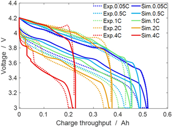
Figure 6. Experimental and simulated successive charge/discharge cycles at 20 °C. Protocol: CC charge (0.05 C, 0.5 C, 1 C, 2 C, 4 C) - fixed 1 C CCCV discharge (cut-off C/20).
Download figure:
Standard image High-resolution imageOverall, the macroscopic electrochemical behavior of the simulated cell agrees well with the experimental data for all the performed protocols, over the entire range of SOCs, C-rates, and temperatures studied. Worth noting, this is achieved with a single set of model parameters. We therefore conclude the general ability of the model to describe the behavior of the present experiments and next use it for predicting aging under additional operating conditions. It is worth noting that the aging model is not necessarily unique, because additional aging mechanisms not included model may also cause or at least contribute to the observed behavior. For example, the aging reactions used in the present model (SEI formation and lithium plating) lead to LLI as only degradation mode, while mechanisms leading to LAM (e.g., decomposition of active material or electrode dry-out) are not included. Still, irreversible lithium plating is typically considered the dominating mechanism for the conditions studied here (charging at fast rates and/or low temperatures). 6,51,52 It is therefore a reasonable simplification not to include additional aging mechanisms.
Aging colormaps
In order to visualize the influence of operation conditions on cell aging, we have introduced before the concept of a aging colormap. 11,21,22 These maps use a color look-up table to show aging (or other cell properties) as function of both temperature and charging current. Often they show a relatively sharp transition between harming and non-harming conditions.
We have carried out systematic simulations over a wide range of temperatures (−20 °C...60 °C in increments of 5 °C) and C-rates (0.05...2 C in increments of 0.5 C). The cell is pre-charged up to 100% SOC with a constant current of 0.02 C, hence simulations start with a CCCV discharge to 3.0 V followed by 30 min rest, a CCCV charge to 4.2 V (cut-off current C/20) and again final 30 min rest. In Fig. 7a the temperature increase  happening during cycling is shown as a function of temperature and C-rate: a slight warming can be observed for the high C-rates, with the cell reaching a +1 °C difference at 2 C and 5 °C. The temperature values represent averages over the cell thickness (x scale in Fig. 2): it should be noted that the predicted temperature gradient along the cell thickness is small (<0.1 °C for all conditions, results not shown) which is due to the small dimension of the investigated cell (3.2 mm thickness). The rather small temporal and spatial temperature gradients would likely allow to omit the thermal scale and use an isothermal aging-sensitive model to get similar results; yet this was not attempted here in order to keep the generalized P3D framework that we have applied before to other, larger cells with higher thermal gradients (e.g., a 26650 cylindrical cell with >10 °C temperature increase at 10 C
40
).
happening during cycling is shown as a function of temperature and C-rate: a slight warming can be observed for the high C-rates, with the cell reaching a +1 °C difference at 2 C and 5 °C. The temperature values represent averages over the cell thickness (x scale in Fig. 2): it should be noted that the predicted temperature gradient along the cell thickness is small (<0.1 °C for all conditions, results not shown) which is due to the small dimension of the investigated cell (3.2 mm thickness). The rather small temporal and spatial temperature gradients would likely allow to omit the thermal scale and use an isothermal aging-sensitive model to get similar results; yet this was not attempted here in order to keep the generalized P3D framework that we have applied before to other, larger cells with higher thermal gradients (e.g., a 26650 cylindrical cell with >10 °C temperature increase at 10 C
40
).
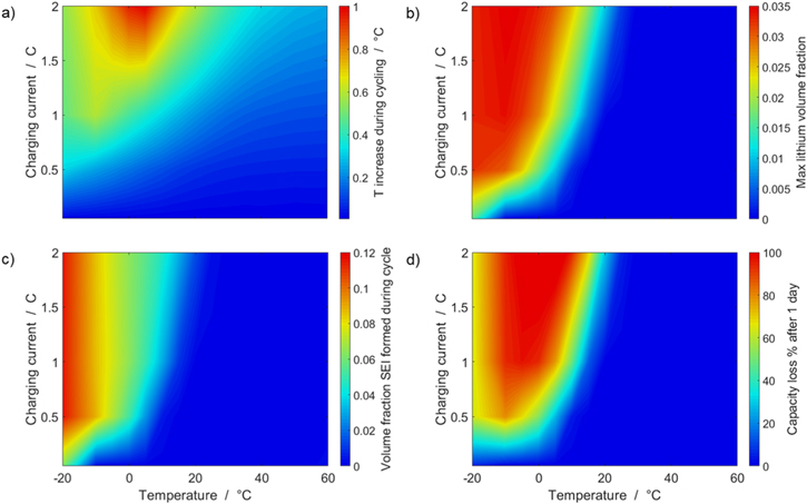
Figure 7. Aging colormaps of a CCCV cycle. (a) Temperature increase during cycling  (b) Peak value of the volume fraction of plated lithium formed, where a value of zero means that no metallic lithium has formed. (c) Peak value of the volume fraction of SEI formed during one cycle, where a value of zero means that no SEI has formed. (d) Capacity loss in % per day (assuming continuous cycling of the battery, as per protocol).
Download figure:
Standard image High-resolution imageFigure 7b shows the maximum lithium volume fraction  reached during cycling as a function of temperature and C-rate. There is a clear transition between no-plating conditions (
 ) and plating conditions, for which
  over a wide range of conditions. For constant C-rate, the transition is relatively sharp for decreasing temperature; at 1 C, it occurs between ca. 5 °C and 15 °C. For constant temperature, the transition is smooth for increasing C-rate; at 20 °C, plating starts above ca. 1.5 C (simulated
  at 20 °C 2 C); at 5 °C, plating starts above ca. 0.2 C.
Figure 7b correlates qualitatively with the experimental results discussed in "Detection of lithium plating", in which an evident voltage plateau was observed in the relaxation curve at 20 °C at 2 C, but not at 1 C or 0.5 C. Also, the long cycling test at 20 °C showed little aging at 1 C, but considerable aging at 2 C. At 5 °C, no voltage plateau was experimentally detected at any of the charging rates (0.5 C, 1 C and 2 C) during the relaxation measurements, while in the simulations plating is clearly predicted (simulated  at 5 °C 2 C): the absence of an experimental plateau could be due to a possible plating irreversibility at this temperature, and/or slow kinetics. However, the increase in cell thickness observed during the short cycling measurements at 5 °C at all investigated C-rates (0.5 C, 1 C, 2 C) ("Detection of lithium plating") does indicate the presence plating, consistent with the simulations.
In Figure 7c the SEI volume fraction  formed within one CCCV cycle is shown: the highest value (∼0.12) is here found at −20 °C for C-rates ≥ 0.5 C, with the SEI produced mainly at low temperatures via the plating-driven reaction (cf. Table I, Reaction 4). This observation correlates well with the previous discussion on the comparison between simulations and cell expansion measurements from "Detection of lithium plating".
Similarly to our previous work, 11 we can also describe aging in a practically meaningful way by converting the predicted SEI formation during the simulated cycle to capacity loss in % per day CLD according to

Here,  are the SEI moles formed during one cycle (summed over the complete NE thickness),
  is the moles of lithium ions bound in one mole of SEI (for LEDC,
 = 2),
= 2),  is the nominal capacity of the cell and ND is the calculated number of cycles in one day (assuming continuous cycling of the battery, as per protocol).
  is directly proportional to the volume fraction of SEI formed during the cycle and, by referring to a fixed amount of cycling time (one day), includes the difference in cycling time for the compared C-rates. Figure 7d shows CLD as a function of temperature (−20 °C...60 °C) and C-rate (0.05...2 C). It shows how easily this particular cell is prone to aging, since almost 100% capacity loss can be already observed after one day of continuous cycling at 1 C at −5 °C (
 = 97%) and a full 100% capacity loss can be found at 2 C for −10 °C ≤ T ≤ 10 °C. As expected from the plating volume fraction
  (Panel a), the limit between aging/no aging zones tends to move towards higher temperatures with increasing C-rates. Different to
  CLD shows decreasing values when further cooling down (∼64% at T = −20 °C for C-rates ≥ 1 C). This is due to the ND factor, which includes in Eq. 1 the time length of CCCV cycles, hence the lower number of cycles per day at low C-rates and at cold temperatures for C-rates ≥ 1 C.
We can now compare qualitatively the long cyclic aging test results presented in "Detection of lithium plating" with simulated values calculated using  from Fig. 7d. At 1 C the experimental capacity was seen decreasing by 0.71% after 50 cycles and a total of 2.80% after 100 cycles, while the simulated cell, when extrapolated from Fig. 7d, would show a higher capacity loss both at 50 cycles (2.6%) and 100 cycles (5.19%). At 2 C the experimental cell experienced a capacity fade of 5.8% after 5 cycles, while the simulated capacity loss would be 12.5%. After 100 cycles the simulation predicts a total failure of the cell (>100% capacity loss), while the experimental capacity fade was observed to be no more than 13.5%. While the simulations follow qualitatively the same trends as the experiments, the quantitative mismatch is obvious. This might be explained as follows. The parameterization of the model has been carried out using accelerated aging experiments down to ca. 30% capacity loss. As shown in Fig. 5, the experimental cell used for those experiments exhibited considerable capacity loss even at 20 °C. This is inconsistent with the experimental long cycling tests. This self-inconsistency of the different experimental data sets leads to the inconsistency of the simulations.
During experimental aging, SEI formation is known to slow down, with different SEI self-passivation mechanisms expected to dominate at different time scales, 53,54 including diffusion-limited film growth and electrolyte consumption (EC is a main reactant in the SEI formation reaction) with increasing cycling time. 8 This effect is not captured in the simulations leading to Fig. 7d. Therefore, the results shown in Fig. 7d represent a cell close to beginning-of-life, where the longer-term cycling effects, including the aforementioned SEI self-passivation, are not captured.
Lithium-ion batteries are also known to exhibit nonlinear aging and develop "knees" towards end-of-life, as has been reviewed recently by Attia et al. 51 This is usually a result of the interaction between several aging mechanisms. The present model would in principle be able to describe such interaction (e.g., the impact of internal resistance increase due to SEI formation on half-cell potential and therefore the plating kinetics), but this would require long-term simulations 8 which is out of scope of the present study. Instead, the capacity loss shown in Fig. 7d is extrapolated from two consecutive simulated cycles of a fresh cell. Therefore, it must be noted again that the simulation results represent the aging behavior of the investigated cell at beginning-of-life.
Aging Indicators
The modeling framework with its aging chemistry illustrated in the previous section has the potential to accelerate the determination of the operating limits for fast charging and to avoid or at least reduce cost- and time-intensive aging experiments. Nevertheless, this approach is computationally expensive, requires dedicated calibration experiments, and due to the conceptual complexity could not be easily included in commercial software tools for industrial applications. A derivation of operating limits from internal states (e.g., NE potential, voltage...) without explicit modeling of aging chemistry, as shown previously, 22,23 would be preferred.
We introduce here different aging indicators derived by post-processing simulations using the SM, a standard physicochemical pseudo-2D "Newman"-type isothermal model (also referred to as Doyle-Fuller-Newman or DFN model) without aging chemistry. 41,42 This model is readily available both in open-source (e.g., PyBAMM 55 ) and commercial (e.g., COMSOL Multiphysics 56 ) software. A number of internal states are available from the SM, including the NE potential, local current density and lithium-ion concentration profiles. The goal of the following study is to develop aging indicators derived from internal states of a SM and validate them by testing against the prediction of the FM. With the term aging indicator we refer to a qualitative measure of capacity loss as function of C-rate and temperature, based on analytical expressions as function of the internal state values available in the SM.
In order to allow for a direct comparison, we have converted our FM to a SM by including only the two intercalation/de-intercalation reactions (cf. Table I, Reactions 1, 5) at the electrodes, while all the other parasitic reactions (lithium plating and SEI formation reactions, cf. Table I, Reactions 2, 3, 4) are switched off. Continuity equations for metallic lithium and SEI are removed. The macroscale (x scale in Fig. 1), which describes the heat transport along the cell thickness and holder plates, is also not included and the simulations are run isothermally.
Figure 8 show six different aging colormaps obtained from six different aging indicators, plotted as a function of temperature (−20 °C...60 °C) and C-rate (0.05...2 C). All aging indicators are dimensionless. All colormaps are based on the same simulation run using the SM. These simulations follow the same protocol from "Aging colormaps", starting at 100% SOC with a CCCV discharge to 3.0 V followed by 30 min rest, then a CCCV charge to 4.2 V (cut-off current C/20) and again final 30 min rest.

Figure 8. Aging colormaps of a CCCV cycle. Six aging indicators (Θ1...Θ6) are obtained from the "simple model" (SM) in which only intercalation/de-intercalation reactions are included and plotted as a function of temperature (−20 °C...60 °C) and C-rate (0.05...2 C). The values are calculated per day (assuming continuous cycling of the battery, as per protocol).
Download figure:
Standard image High-resolution imageWe refer to the first and simplest aging indicator Θ1 as "Thermodynamics with constant plating condition." It is shown in Fig. 8a. It is given as,

where,  is the NE potential averaged over the complete NE thickness and the integrals run over the complete duration of charging. NSM is the calculated number of cycles in one day (assuming continuous cycling of the battery, as per protocol), normalized to a reference value at 20 °C and 1 C (needed to keep Θn
dimensionless). This factor is used to include the difference in cycling time for the compared C-rates and temperatures and makes the indicator relative to time, instead of number of cycles. The aging indicator (without the NSM factor) was used before by Tippmann
22
: it assumes that plating takes place as soon as the thermodynamic plating condition (
is the NE potential averaged over the complete NE thickness and the integrals run over the complete duration of charging. NSM is the calculated number of cycles in one day (assuming continuous cycling of the battery, as per protocol), normalized to a reference value at 20 °C and 1 C (needed to keep Θn
dimensionless). This factor is used to include the difference in cycling time for the compared C-rates and temperatures and makes the indicator relative to time, instead of number of cycles. The aging indicator (without the NSM factor) was used before by Tippmann
22
: it assumes that plating takes place as soon as the thermodynamic plating condition ( drops below 0 V) is fulfilled. The capacity (the current integrated) charged under this condition is normalized to the total capacity during charge. A value of
  means that the NE potential stays below zero during the complete charging process.
The second aging indicator Θ2 is referred to as "Thermodynamics with dynamic plating condition," shown in Fig. 8b. Here we use a modified expression according to

where,  is the equilibrium voltage of the plating reaction (Table I, Reaction 2). We have suggested this expression before.
21
It is based on the assumption that the plating thermodynamics is not fixed to 0 V, but varies along the cycle depending on temperature and (local) lithium-ion concentration
is the equilibrium voltage of the plating reaction (Table I, Reaction 2). We have suggested this expression before.
21
It is based on the assumption that the plating thermodynamics is not fixed to 0 V, but varies along the cycle depending on temperature and (local) lithium-ion concentration  in the electrolyte. The values for
  are here calculated using the Nernst equation

where,  is the standard Gibbs energy of reaction for lithium metal, which is a function of temperature, but not of concentration, and
  is the mole fraction of lithium ions in the electrolyte, averaged over the complete NE thickness (see Ref. 39).
  can be calculated from the standard-state chemical potential
  according to

where,  and
and  are respectively the molar enthalpy and molar entropy for lithium metal. Molar enthalpies and entropies as function of temperature have been compiled in form of polynomial functions for a large number of compounds in the NASA thermochemical tables:
57
we refer the reader to Ref. 21, 47 for a detailed explanation about the subject. Θ2 is normalized to the total charge throughput during charging, i.e., a value of Θ2 = 1 means that the NE potential stays below the plating equilibrium potential
are respectively the molar enthalpy and molar entropy for lithium metal. Molar enthalpies and entropies as function of temperature have been compiled in form of polynomial functions for a large number of compounds in the NASA thermochemical tables:
57
we refer the reader to Ref. 21, 47 for a detailed explanation about the subject. Θ2 is normalized to the total charge throughput during charging, i.e., a value of Θ2 = 1 means that the NE potential stays below the plating equilibrium potential  during the complete charging process.
Chemical reactions are not driven by thermodynamics alone. Instead, kinetics play a key role, in particular when comparing different temperatures. For the third aging indicator Θ3, shown in Fig. 8c, we therefore include the kinetics in addition to the thermodynamics. We refer to it as 'Plating vs intercalation kinetics', considering the formation rates of metallic lithium  and intercalated lithium
  (given in mol m−3 s−1) according to,

Here, the integrals run over positive values of the formation rates. The integrals take the role of continuity equations, giving the total formed concentrations of lithium metal and intercalated lithium, respectively. This indicator was used previously
21
(without the NSM factor). The species formation  are calculated via the Butler-Volmer equation
with

where,  is calculated via Eq. 4 for the plating reaction, and
  is the NE potential averaged over the complete NE thickness. The values for
  and
and  can be found respectively in Tables I and VI (Appendix). About the equations for the calculation of
  in Eq. 7, we refer the reader to the Appendix. The aging indicator Θ3 is obtained by integrating
  and dividing it by the sum of the integrated
  and
and  both only for positive rates of formation: this gives us the ratio of plated lithium to the total amount of lithium involved in the reactions at the NE (intercalated and plated). A value of Θ3 = 1 means that only plating is taking place and no intercalation.
Figure 8d shows a colormap for the fourth aging indicator Θ4, referred to as "Accumulated lithium" and defined as

Here,  is the fixed ratio of molar mass and density of metallic lithium (cf. Table V in the Appendix). Instead of considering lithium metal formation relative to total formation rates as in Θ3, this factor considers the plating reaction only. In fact, Eq. 9 represents a continuity equation for lithium metal, and Θ4 is proportional to the maximum lithium volume fraction during cycling
  As a result of the
  factor, a value of Θ4 = 1 means that the complete electrode consists of lithium only.
All the aging indicators presented until now focus on plating as main cause of damage for the cell. However, as we have shown above, the cell degradation does not result from plating alone (which is fully reversible), but from the consequent reaction of plated lithium with electrolyte to SEI. For the fifth indicator Θ5 (Fig. 8e), we therefore include a contribution of the plating-driven SEI formation (cf. Table I, Reaction 4) and refer to it as "Accumulated lithium plus SEI." Here we simply use the temperature-dependent part of SEI formation, by multiplying Θ4 with an Arrhenius factor according to
where,  is the activation energy according to Table I, Reaction 4. Because of the Arrhenius factor completely changing the order of magnitude, we decided here to use a temperature of 20 °C as reference, in order to keep the concept of nondimensionalization and relative values.
The indicator Θ5 remains proportional to  However, SEI formation is a dynamic process. It can be assumed that a low amount of lithium metal over a long period of time causes similar aging than a high amount of lithium metal over a short period of time. To consider this, we finally introduce the sixth aging indicator Θ6, labelled "Coupled lithium and SEI" and shown in Fig. 8f. Here we assess the evolution of plated lithium during time as well as the contribution from the plating-driven SEI formation, according to
Here,  is the fixed ratio of molar mass and density of LEDC (cf. Table V in the Appendix),
  is the rate coefficient of the plating-driven SEI formation (cf. Table I, Reaction 4) and
  is the mole fraction of ethylene carbonate (C3H4O3) in the electrolyte (see Ref. 39). The inner integral runs only over positive values of the plated lithium formation rate, while the outer integral runs over the complete duration of the cycle. The inner integral represents the continuity equation for lithium metal, while the outer integral represents the continuity equation for SEI.
We next discuss the behavior of these six aging indicators shown in Fig. 8. All indicators show a qualitatively similar behavior, with the limit between aging/no aging zones moving towards higher temperatures with increasing C-rates and a general harming situation found at T < 20 °C for C-rates > 1 C. Nevertheless, some discrepancies can be observed between the plots. Θ1 and Θ2 (Panels a,b) are dominated by plating thermodynamics and both show severe aging for −5 °C ≤ T ≤ 20 °C, with a maximum aging at 15 °C and 2 C (0.82 and 0.92 for Θ1 and Θ2, respectively). The most pessimistic results are found for Θ3 (Panel c), in which the lower activation energy for the plating reaction (compared to intercalation: ∼65 kJ vs ∼75 kJ), combined to the lack of normalization for both  to the initial volume fractions (included in the FM), could cause a possible overestimation of the simulated damage: here totally "safe" conditions for fast charging ( ≥ 1 C) are present only when T ≥ 30 °C and a significant damage can be found at 0 °C ≤ T ≤ 15 °C at 1 C and −5 °C ≤ T ≤ 25 °C at 2 C (Θ3 = 1 at 10 °C ≤ T ≤ 20 °C). Θ4 and, even more so, Θ5 (Panels d,e) show lower aging values compared to the previous ones on the 0...1 scale, with no red zones and a maximum aging at 10 °C and 2 C (0.65 and 0.60 for Θ1 and Θ2, respectively). Finally, Θ6 shows some important differences to the previous indicators, with a harming zone shifted towards lower temperatures (−15 °C ≤ T ≤ 10 °C at 2 C and between −15 °C and 0 °C at 1 C) and a maximum at -5 °C and 2 C (∼0.09). Worth noting, for all indicators the highest values do not occur at the lowest T, a fact which reflects the slowdown kinetics of plating and SEI formation with decreasing temperature, and reminds of what was observed for the FM in Fig. 7d. This is due to the NSM factor, which includes in all the Θn
equations the time length of CCCV cycles, hence the lower number of cycles per day at low C-rates and at cold temperatures for C-rates ≥ 1 C.
to the initial volume fractions (included in the FM), could cause a possible overestimation of the simulated damage: here totally "safe" conditions for fast charging ( ≥ 1 C) are present only when T ≥ 30 °C and a significant damage can be found at 0 °C ≤ T ≤ 15 °C at 1 C and −5 °C ≤ T ≤ 25 °C at 2 C (Θ3 = 1 at 10 °C ≤ T ≤ 20 °C). Θ4 and, even more so, Θ5 (Panels d,e) show lower aging values compared to the previous ones on the 0...1 scale, with no red zones and a maximum aging at 10 °C and 2 C (0.65 and 0.60 for Θ1 and Θ2, respectively). Finally, Θ6 shows some important differences to the previous indicators, with a harming zone shifted towards lower temperatures (−15 °C ≤ T ≤ 10 °C at 2 C and between −15 °C and 0 °C at 1 C) and a maximum at -5 °C and 2 C (∼0.09). Worth noting, for all indicators the highest values do not occur at the lowest T, a fact which reflects the slowdown kinetics of plating and SEI formation with decreasing temperature, and reminds of what was observed for the FM in Fig. 7d. This is due to the NSM factor, which includes in all the Θn
equations the time length of CCCV cycles, hence the lower number of cycles per day at low C-rates and at cold temperatures for C-rates ≥ 1 C.
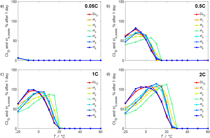
Figure 9. Comparison of the capacity loss CLD predicted by the FM with the aging indicators  derived from the SM in % per day, plotted as a function of temperature (−20 °C...60 °C) for different C-rates. In (a) 0.05 C, (b) 0.5 C, (c) 1 C and (d) 2 C.
Download figure:
Standard image High-resolution imageThe aging indicators were calculated with the SM. In order to assess their validity, we compare them to the output of the FM (cf. Fig. 7d and Table I) in a model-to-model comparison. To quantify the performance of the indicator approach, we normalize the  to our reference indicator
  from the FM according to

where,  and
and  are the mean values over T for the different aging indicators at each C-rate. The indicators
  normalized such represent capacity loss in the unit of % per day. The results are plotted vs
  in Fig. 9 at 0.05 C (a), 0.5 C (b), 1 C (c) and 2 C (d) as function of temperature between −20 °C and 60 °C. At 0.05 C (Panel a) no aging is really visible (except at −20 °C), while values rise evidently at C-rates ≥ 0.5 C. If we compare the various indicators with
  (red curve), we can notice how
  tends to strongly overestimate aging over 0 °C, 5 °C and 10 °C respectively in Figs. 9b–9d, as well as
  and
and  curves have their maximum shifted by +10 °C compared to
  The
The  and
and  curves look shifted to the right too, but show a better simulation towards the decrease at the lowest temperatures.
  looks the best one, nearly superimposing the red curve in every panel (especially at 0.5 C and 1 C).
For a better comparison, we introduce a "Goodness of Indicator" (GoI) factor,

where,  is the number of temperatures analyzed in the GoI. The results are given in Table II, where lowest GoI values indicate the highest similarity between
  and the reference
  From these data,
  is clearly the most accurate indicator derived from the SM and the best "simple" approach to quantitatively evaluate operating limits for the analyzed cell.
Table II. GoI for  as a function of temperature (−20 °C...60 °C) and C-rate (0.05...2 C).
| GoIn | 0.05 C | 0.5 C | 1 C | 2 C |
|---|---|---|---|---|
| Θ1Thermodynamics (constant plating) | 0.06 | 2.75 | 5.05 | 12.98 |
| Θ2Thermodynamics (dynamic plating) | 0.05 | 4.99 | 10.60 | 17.24 |
| Θ3Plating vs intercalation kinetics | 0.20 | 10.31 | 16.68 | 25.90 |
| Θ4Accumulated lithium | 0.03 | 2.62 | 5.17 | 9.37 |
| Θ5Accumulated lithium plus SEI | 0.03 | 3.80 | 7.24 | 12.74 |
| Θ6Coupled lithium and SEI | 0.05 | 1.03 | 1.09 | 2.05 |
Conclusions
We have presented the development, parameterization and application of a pseudo-three-dimensional (P3D) aging model ("full model") of a lithium-ion cell with graphite negative and NMC positive electrode. A systematic approach towards parameterization was used, starting from equilibrium and then adding transport processes on all three scales as well as electrochemistry. Electrochemical reactions for SEI formation on graphite, lithium plating, and SEI formation on plated lithium are included, with the aging model assessing the positive feedback of plating on SEI growth and thus being able to describe cell aging over a wide temperature range. As expected, the presence of plated lithium accompanies a correspondent higher SEI formation, hence a more evident capacity loss during cycling. The model was validated against experiments in the frequency domain (using EIS) and time domain (using discharge/charge cycling) over a wide range of SOC, C-rates and temperatures, with simulations showing a good qualitative agreement with experimental data for all the different protocols applied.
This model allows to quantify capacity loss due to cycling (here in % per day) as function of operating conditions and the visualization of various aging colormaps as function of both temperature and C-rate (0.05 to 2 C charge and discharge, −20 °C to 60 °C). When the SEI formation combines with plating at low temperatures, a significant capacity loss can happen especially for high C-rates. The limit between plating/no plating zones moves towards higher temperatures with increasing C-rates, while very low temperatures and high C-rates reduce the cyclable SOC range: this reduces both the SEI growth and the plating, leading to lower aging values in the harshest conditions. The model predictions on plating and SEI formation were qualitatively confirmed through voltage relaxation and cell expansion measurements, while the predicted capacity loss during cycling at 20 °C was found to be considerably higher than observed in long-term cycling experiments. This inaccuracy might be due to a too "pessimistic" parameterization of the plating-driven SEI formation reaction, which leads to an overprediction of the plating irreversibility and a subsequent exaggerated SEI formation. Worth noting, the aging kinetics were parameterized to accelerated aging experiments down to ca. 30 % capacity loss, and not to long-term cycling data. The model prediction thus represents the cell behavior at beginning-of-life.
In the second part of the paper, six different aging indicators Θn for determination of operating limits in fast charging, derived from postprocessing simulations of a standard physicochemical pseudo-two-dimensional (P2D) "Newman-type" isothermal model without aging mechanisms ("simple model"), are introduced: a number of internal states are available for this purpose, including the NE potential, local current density and lithium-ion concentrations. The "simple model" includes only the two intercalation/de-intercalation reactions at the electrodes, while all the other parasitic reactions are switched off. The aging indicators were normalized to the capacity loss in % per day previously obtained from the P3D aging model and evaluated using a specifically developed "Goodness of Indicator" (GoI) factor. A particularly good result was obtained for Θ6, an aging indicator which assesses the evolution of plated lithium formation during time as well as the contribution from the plating-driven SEI formation.
This study is to be considered a modeling framework for determining fast-charge limits, both using detailed physicochemical aging models, and simplified aging indicators which can be included in open-source or commercial software tools for industrial applications. The framework represents the aging behavior at beginning-of-life; nonlinear aging, SEI self-slow-down and the development of "knees" towards end-of-life 51 are not predicted. Long-term simulations with the model framework should be subject of future studies, in particular given the observed disagreement of the beginning-of-life prediction with experimental long-term (100 cycles) aging tests.
CRediT author statement
Serena Carelli: Conceptualization, Methodology, Validation, Writing - Original draft preparation. Yan Ying Lee: Investigation, Writing - Original draft preparation. André Weber: Writing—Review and Editing, Supervision, Funding acquisition. Wolfgang G. Bessler: Conceptualization, Software, Writing—Review and Editing, Supervision, Funding acquisition.
Acknowledgments
This work was carried out in the framework of the German industrial collective research programme (IGF, grant no. 20882 N/2). It was supported by the Federal Ministry for Economic Affairs and Climate Action (BMWK) through the AiF (German Federation of Industrial Research Associations eV) based on a decision taken by the German Bundestag. The authors thank the German Research Association for Power Transmission Engineering (FVA).
Appendix
A short model description and a summary of all model equations and parameters, as well as symbol definitions, are given in this appendix. We also present a systematic approach towards model parameterization, along with a compilation of the required materials properties.
Appendix. Modeling domain and main assumptions
The model features a pseudo-3D domain (cell scale, electrode pair scale, particle scale), see Fig. 2. All model equations are given in Table III. A list of symbols is provided . On the cell level (x scale in Fig. 2), heat transport is modeled in one dimension as conduction along the cell thickness and holder plates, using convective and radiative heat transfer as boundary conditions. This dimension runs perpendicular to the electrode sheets of the pouch cell. On the electrode pair level (y scale in Fig. 2), mass and charge transport of Li+ and PF6 – ions in the liquid electrolyte and electrons in the solid electrode components is modeled in one dimension along the thickness of the electrode pair. Again, this is perpendicular to the electrode sheet area. For ion transport, we describe species fluxes due to migration and diffusion with a Nernst-Planck approach with concentration- and temperature-dependent diffusion coefficients. Electronic conductivity within the electrodes is assumed high and not rate-limiting. On the particle level (z scale in Fig. 2), the diffusion of intercalated lithium atoms in the bulk of the AM particles is modeled using a simple Fickian diffusion approach. The diffusion coefficients are assumed concentration and temperature dependent.
Table III. Summary of all model equations.
| Macroscale (x direction): Heat transport in cell | |
|---|---|
| Energy conservation |
|
| Heat flux at cell surface |

|
| Total heat sources |

|
| Chemistry heat source |

|
| Ohmic heating |

|
| Mesoscale (y direction): Mass and charge transport in electrode pair | |
|---|---|
| Mass conservation of species i |

|
| Charge conservation |
|
| Species fluxes (Nernst-Planck) |
|
| Microscale (z direction): Mass transport in active materials particle | |
|---|---|
| Mass conservation (Fick's 2nd law) |
|
| Chemical kinetics and thermodynamics a) | |
|---|---|
| Energy conservation |

|
| Heat flux at cell surface |

|
| Total heat sources |
|
| Chemistry heat source |
|
| Ohmic heating |
|
| Mesoscale (y direction): Mass and charge transport in electrode pair | |
| Mass conservation of species i |
|
| Charge conservation |

|
| Species fluxes (Nernst-Planck) |

|
| Microscale (z direction): Mass transport in active materials particle | |
| Mass conservation (Fick's 2nd law) |

|
| Chemical kinetics and thermodynamics a) | |
| Interfacial rate of electrochemical reaction n (Butler-Volmer) |
![${{\boldsymbol{r}}}_{{\boldsymbol{n}}}=\displaystyle \frac{{{{\boldsymbol{i}}}_{{\boldsymbol{n}}}}^{0}}{{\boldsymbol{F}}}\left[\exp \left(\displaystyle \frac{{{\boldsymbol{\alpha }}}_{{\bf{c}}}{\boldsymbol{zF}}}{{\boldsymbol{RT}}}{{\boldsymbol{\eta }}}_{{\bf{a}}{\bf{c}}{\bf{t}},{\boldsymbol{n}}}\right)-\exp \left(-\displaystyle \frac{\left(1-{{\boldsymbol{\alpha }}}_{{\bf{c}}}\right){\boldsymbol{zF}}}{{\boldsymbol{RT}}}{{\boldsymbol{\eta }}}_{{\bf{a}}{\bf{c}}{\bf{t}},{\boldsymbol{n}}}\right)\right]$](https://content.cld.iop.org/journals/1945-7111/170/2/020525/revision2/jesacb8e1ieqn173.gif)
|
| Exchange current density |
|
| Overpotential |

|
| Interfacial rate of thermochemical reaction n (mass-action kinetics) |
|
| Forward rate constant |
|
| Reverse rate constant |
|
| Species source terms |
|
| Equilibrium potential (Nernst equation) |
|
| Gibbs reaction energy |
|
| Standard-state chemical potential |
|
| Current, voltage, potentials | |
| Cell voltage |

|
| Cell current |
|
| Faradaic current density |
|
| Double layer current density |

|
| Species source term from double layer |
 with with 
|
| Potential step (both electrodes) |

|
| Multi-phase management | |
| Volume fraction of phases |
|
| Feedback on transport coefficients (porous electrode theory) |

|
| Current, voltage, potentials | |
|---|---|
| Cell voltage |
|
| Cell current |

|
| Faradaic current density |

|
| Double layer current density |

|
| Species source term from double layer |
 with with 
|
| Potential step (both electrodes) |

|
| Multi-phase management | |
|---|---|
| Volume fraction of phases |
|
| Feedback on transport coefficients (porous electrode theory) |

|
The model framework includes continuity equations for all solid, liquid and gaseous phases present in the electrode, allowing to track formation and growth of new phases. In the continuum setting, all phases are characterized by their respective volume fractions. Lithium metal and LEDC are both included as solid phases at the NE, and their starting volume fractions are respectively set to an initial value of 10−11 and 8·10−4. As SEI and metallic lithium grow, the electrode porosity is reduced accordingly.
The chemical thermodynamics and kinetics are calculated with the Cantera software suite (version 2.5.0a3).
44
Details on the use of Cantera for lithium-ion batteries are given by Mayur et al.
47
For the thermodynamics of the two AM (NMC, graphite) we use Cantera's BinarySolutionTabulatedThermo class. The electrolyte phase is described through the IdealSolidSolution class, with the standard concentration set to a unity value. Both Li[metal] and ![${({\bf{C}}{{\bf{H}}}_{2}{\bf{O}}{\bf{C}}{{\bf{O}}}_{2}{\bf{L}}{\bf{i}})}_{2}\left[{\bf{S}}{\bf{E}}{\bf{I}}\right]$](https://content.cld.iop.org/journals/1945-7111/170/2/020525/revision2/jesacb8e1ieqn201.gif) species are described through Cantera's StoichSubstance class (stoichiometric_solid). For the kinetics, note Table I contains both electrochemical and thermochemical reactions, which are treated within the consistent framework provided by Cantera's interfaceKinetics class. Kinetics involving solid phases, such as metallic lithium, require special attention: thermodynamically, the activity of solid phases is unity regardless of the amount of solid. However, reaction kinetics must go to zero if the phase vanishes. This is not considered with standard mass-action kinetics. In the present model, we define for metallic lithium a limiting volume fraction of 10–10, below which the decomposition rate is set to zero. For this we use Cantera's phaseExistence functionality implemented in the interfaceKinetics class. During right-hand side calculation, we set the phaseExistence flag to false if the volume fraction is below 10–10, causing Cantera to set the reaction rate to zero. The Cantera input file is available from the authors upon request.
species are described through Cantera's StoichSubstance class (stoichiometric_solid). For the kinetics, note Table I contains both electrochemical and thermochemical reactions, which are treated within the consistent framework provided by Cantera's interfaceKinetics class. Kinetics involving solid phases, such as metallic lithium, require special attention: thermodynamically, the activity of solid phases is unity regardless of the amount of solid. However, reaction kinetics must go to zero if the phase vanishes. This is not considered with standard mass-action kinetics. In the present model, we define for metallic lithium a limiting volume fraction of 10–10, below which the decomposition rate is set to zero. For this we use Cantera's phaseExistence functionality implemented in the interfaceKinetics class. During right-hand side calculation, we set the phaseExistence flag to false if the volume fraction is below 10–10, causing Cantera to set the reaction rate to zero. The Cantera input file is available from the authors upon request.
Appendix. Model parameterization
Approach
The parameterization of electrochemical models is one of the key factors in building up a reliable and working model, given the number of parameters and their dependence on operating conditions. In particular, we require (1) thermodynamic data of all species involved (molar enthalpies and entropies including their dependence on lithium stoichiometry in case of intercalation materials); (2) kinetic data of all reactions (pre-exponential factors, activation energies and symmetry factors); (3) physical data of all phases (phase densities or species molar volumes); and (4) structural parameters (electrode thicknesses, volume fractions, etc.). For a detailed description of the experimental methodology, see "Experimental Methodology".
Cell at thermodynamic equilibrium
The base parameters needed for the lithium-ion battery model are those that are associated with the thermodynamic equilibrium, that is, that describe the open-circuit voltage  as function of charge throughput
  Parameters related to nonequilibrium effects such as transport on multiple scales and finite reaction kinetics can only be identified reliably if the equilibrium behavior is modeled correctly.
We start by collecting molar thermodynamic properties (molar enthalpies ![${{\boldsymbol{h}}}_{{\bf{L}}{\bf{i}}[{\bf{A}}{\bf{M}},{\boldsymbol{i}}]}^{0}$](https://content.cld.iop.org/journals/1945-7111/170/2/020525/revision2/jesacb8e1ieqn204.gif) and molar entropies
and molar entropies ![${{\boldsymbol{s}}}_{{\bf{L}}{\bf{i}}[{\bf{A}}{\bf{M}},{\boldsymbol{i}}]}^{0}$](https://content.cld.iop.org/journals/1945-7111/170/2/020525/revision2/jesacb8e1ieqn205.gif) ) of intercalated lithium in NMC and graphite. They are obtained from our own experiments of half-cell potential vs lithium metal
) of intercalated lithium in NMC and graphite. They are obtained from our own experiments of half-cell potential vs lithium metal  and from literature data of stoichiometry values (
![${{\boldsymbol{X}}}_{{\bf{L}}{\bf{i}}[{\bf{A}}{\bf{M}},{\boldsymbol{i}}]}$](https://content.cld.iop.org/journals/1945-7111/170/2/020525/revision2/jesacb8e1ieqn207.gif) vs
vs  - shown in Fig. 10a) and temperature dependence
  including a correction for the entropy of the lithium metal counter electrode.
47
Data were selected and processed for NMC
58,59
and graphite
60,61
and the resulting molar thermodynamic data are shown in Fig. 10b. We furthermore collected molar thermodynamic data for all other species present in the model, which are summarized in Table IV and form the thermochemical basis of the model.
including a correction for the entropy of the lithium metal counter electrode.
47
Data were selected and processed for NMC
58,59
and graphite
60,61
and the resulting molar thermodynamic data are shown in Fig. 10b. We furthermore collected molar thermodynamic data for all other species present in the model, which are summarized in Table IV and form the thermochemical basis of the model.
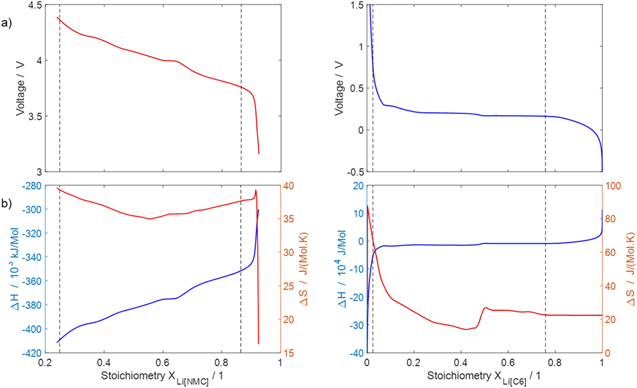
Figure 10. (a) Half-cell potentials (from our own experiments and literature data, 58,60 of stoichiometry values) as well as (b) molar enthalpies and entropies, 59,61 of intercalated lithium at 20 °C, respectively for NMC (left) and graphite (right). The vertical dashed lines indicate the stoichiometry ranges for every AM used in the full cell, as obtained through optimization. See text and Ref. 62 for details.
Download figure:
Standard image High-resolution imageTable IV. Thermodynamic properties of all species included in the model.
| Species | Molar enthalpy  /kJ·mol−1 /kJ·mol−1
| Molar entropy  /J·mol−1·K−1 /J·mol−1·K−1
| References |
|---|---|---|---|
| Li[NMC] | See Fig. 10b (left) | See Fig. 10b (left) | 58, 59 |
| V[NMC] | 0 | 0 | Reference value |
| Li[C6] | See Fig. 10b (right) | See Fig. 10b (right) | 28, 29 |
| V[C6] | 0 | 0 | Reference value |
| LEDC[SEI] | −1383 | 90.07 | Calculated 63 assuming SEI formation potential of 0.8 V vs Li/Li+ |
| C2H4 | 52 a) | 219 a) | 57 |
| Li[metal] | 0 | 29.12 | 21, 47 |
| C3H4O3[elyt] | −578 a) | 175 a) | 57 |
| C4H8O3[elyt] | 0 | 0 | Dummy value (not chemically active) |
 [elyt] [elyt] | 0 | 0 | Reference value |
 [elyt] [elyt] | 0 | 0 | Dummy value (not chemically active) |
a)Values are assumed T-dependent57, here given at 298 K.
Apart from the chemical thermodynamics, the  behavior depends on the available electrode capacity and electrode balancing, which are governed by electrode volume, volume fraction of AM, density of AM, and the stoichiometry range the AM are cycled in. Here we apply the methodology developed by Mayur et al.
62
for self-consistent parameter identification: the resulting parameters are included in Table V and Fig. 10. Furthermore, Table V defines all phases and species assumed in both electrodes and separator.
behavior depends on the available electrode capacity and electrode balancing, which are governed by electrode volume, volume fraction of AM, density of AM, and the stoichiometry range the AM are cycled in. Here we apply the methodology developed by Mayur et al.
62
for self-consistent parameter identification: the resulting parameters are included in Table V and Fig. 10. Furthermore, Table V defines all phases and species assumed in both electrodes and separator.
Table V. Properties of all bulk phases included in the model.
| Layer | Phase | Initial volume fraction 
| Density  /kg·m–3 /kg·m–3
| Species (initial mole fraction X) |
|---|---|---|---|---|
| PE | NMC | 0.456 | 2500 | Li[NMC], V[NMC] (depends on SOC) |
| Electrolyte | 0.357 | 1270 39 | C3H4O3 [elyt] (0.52), C4H8O3 [elyt] (0.34),  [elyt] (0.07), [elyt] (0.07),  [elyt] (0.07) [elyt] (0.07) | |
| Gas phase | 0.080 | From ideal gas law | N2 (1) | |
| Electron conductor | 0.107 | 2000 | No chemically active species | |
| Separator | Separator | 0.5 67 | 777 | |
| Electrolyte | 0.470 | 1270 | same as at PE | |
| Gas phase | 0.030 | From ideal gas law | N2 (1) | |
| NE | C6 | 0.308 | 2270 | Li[C6],V[C6] (depends on SOC) |
| Electrolyte | 0.335 | 1270 | same as at PE | |
| LEDC | 0.0008 | 1300 68 | (CH2OCO2Li)2 | |
| Lithium carbonate | 0.0092 | 2100 | Li2CO3 | |
| Lithium metal | 10-11 | 534 69 | Li | |
| Electron conductor | 0.267 | 2000 | No chemically active species | |
| Gas phase | 0.080 | 1.14 70 | N2 (0.99), C2H4 (0.01) |
Geometry and transport parameters
All geometry and transport parameters of the modeling domain at macro-, meso- and microscale are summarized in Table VI.
Table VI. Geometry and transport parameters of the P3D modeling domain.
| Parameter | Value | References |
|---|---|---|
| Cell thickness | 3.2 mm | Measured |
| Aluminum plate (right/left) thickness | 10 mm | Measured |
Active electrode area 
| 0.030767 m2 | Measured |
Cell thermal conductivity 
| 0.9 W·m–1·K–1 | 39,71 |
Aluminum plate (right/left) thermal conductivity 
| 237 W·m–1·K–1 | 39,72 |
Cell heat capacity 
| 0.95 J·g–1·K–1 | 39,73 |
Aluminum plate (right/left) heat capacity 
| 0.897 J·g–1·K–1 | 39,72 |
Heat transfer coefficient 
| 157 W·m–2·K–1 | Measured 39 |
| Thickness of PE | 84.0 μm | Measured |
| Thickness of separator | 16.0 μm | Measured |
| Thickness of NE | 92.0 μm | Measured |
Tortuosity of PE 
| 1.29 | Bruggeman relationship (calc.) |
Tortuosity of separator 
| 1.21 | Bruggeman relationship (calc.) |
Tortuosity of NE 
| 1.31 | Bruggeman relationship (calc.) |
Diffusion coefficients 

| See Eqs. 14 and 15 | 39,40,63 |
Specific surface area NMC/electrolyte 
| 1.07 ·106 m2 m−3 |

|
Specific surface area graphite/electrolyte 
| 6.94 · 105 m2 m−3 |

|
NE double layer capacitance 
| 3.0·10-2 F·m2 | Fitted to EIS data |
PE double layer capacitance 
| 1.8·10-2 F·m2 | Fitted to EIS data |
Ohmic resistance of current collection system 
| 9.0·10-1 mΩ·m2 | Fitted to EIS data |
Electrical conductivity of the SEI layer 
| 1.0·10-5 S m−1 | Assumed 74 |
Graphite stoichiometry range ![${X}_{{\rm{Li}}\left[{{\rm{C}}}_{6}\right]}$](https://content.cld.iop.org/journals/1945-7111/170/2/020525/revision2/jesacb8e1ieqn238.gif) (0...100% SOC) (0...100% SOC) | 0.025...0.7584 | Optimization |
NMC stoichiometry range ![${X}_{{\rm{Li}}\left[{\rm{NMC}}\right]}$](https://content.cld.iop.org/journals/1945-7111/170/2/020525/revision2/jesacb8e1ieqn239.gif) (0...100% SOC) (0...100% SOC) | 0.8647...0.2488 | Optimization |
Radius of PE particles 
|

| Measured |
Diffusion coefficient of Li in NMC 
| See Fig. 11a | Measured 64 + activation energy 65 |
Radius of NE particles 
|

| Measured |
Diffusion coefficient of Li in graphite 
| See Fig. 11b | Measured 66 + activation energy 60 |
We assume the electrolyte to be composed of EC, EMC, and LiPF6; the exact composition is unknown. We use an electrolyte transport model based on dilute solution theory, 40 but use concentration-dependent diffusivities (accounting for the interaction between the ions in the concentrated solution). The expressions for the ion diffusion coefficients are
We refer the reader to our previous works
39,40,63
for a detailed description of our electrolyte transport model. We also assume an Arrhenius-type dependence on temperature and an activation energy of  = 32.0 kJ mol−1.
Lithium diffusion inside the AM strongly influences cell behavior. Figure 11 shows diffusion coefficients of intercalated lithium as function of intercalation stoichiometry for the two AM. We applied a literature research for concentration- and temperature-dependent diffusion coefficients: for NMC, we chose the work from Noh et al., 64 shown in Fig. 11a, where GITT experiments have been conducted over a nearly complete intercalation stoichiometry range. We included an Arrhenius temperature dependence with an activation energy of 45.45 kJ mol−1 as found by Cui et al. 65 For graphite, we took as reference the work from Levi, 66 where the diffusion was investigated using both PITT and EIS techniques. The values are shown in Fig. 11b. They were also used in the models by Kupper 40 and in our previous works. 11,21,39 An activation energy of 44.0 kJ mol−1 was used, as average between the two values experimentally measured in Ecker et al. 60

Figure 11. Solid-state diffusion coefficients of lithium within (a) NMC and (b) graphite at 20 °C.
Download figure:
Standard image High-resolution imageElectrochemical parameters and SEI model
The electrochemical parameters include the exchange current density factors  and activation energies
  of the two charge-transfer reactions (NMC and graphite) as well as double-layer capacitances of both electrodes. These parameters were obtained by fitting simulated EIS data to experimental values at two different SOC (20%, 50%) and three different temperatures (5 °C, 20 °C, 35 °C). The activation energies were obtained from Arrhenius plots. The resulting values of the double layer capacitances are included in Table VI, while the reaction mechanism and rate coefficients for all AM are reported in Table I.
A comparison of EIS simulations (after parameter fitting) and measurements is shown in Fig. 12. Simulations were carried out for frequencies from 10-2 Hz up to 105 Hz, SOCs of 20%, 35%, 50%, 65%, 80% and 100%, and temperatures of 5 °C, 20 °C, 35 °C and 50 °C. Both experiments and simulations show two features: (i) a small flattened semi-circle at high frequency (between 10 Hz and 100 Hz) which can be assigned to the PE charge-transfer reaction and double layer, overlapped within a larger semi-circle at medium frequency which can be assigned to the NE charge-transfer reaction and double-layer; (ii) a Warburg-type feature at low frequency (< 0.1 Hz) which can be assigned to lithium diffusion in the AM. There is qualitative agreement between model and experiment, except for 5 °C in Panel a) and generally SOC 100% at all temperatures.
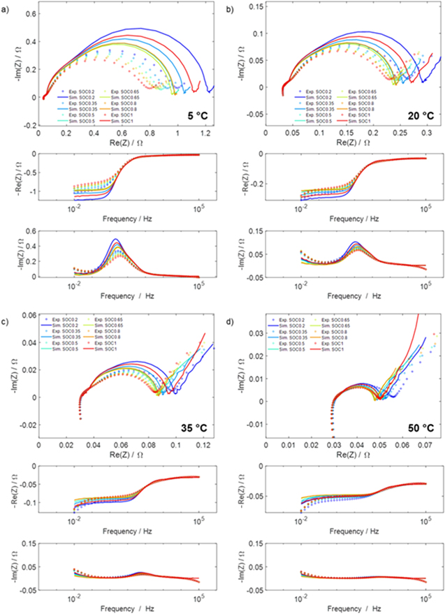
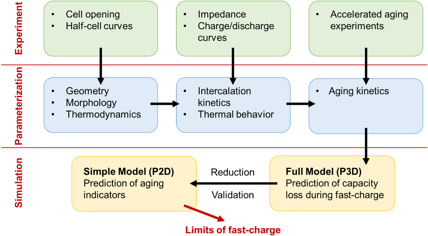
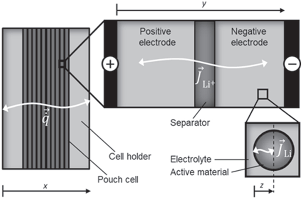
Figure 12. Experimental and simulated electrochemical impedance spectra for varying SOC at different temperatures (a) 5 °C, (b) 20 °C, (c) 35 °C and (d) 50 °C in both Nyquist and Bode representations.
Download figure:
Standard image High-resolution image
About the SEI model, several parameters are needed to simulate both calendaric and cyclic SEI formation, cf. Kupper et al. 8 The applied rate expression is given in Table I (Eq. 3). The SEI thickness is calculated as

The current density during charge is

The derivative of the tangential SEI stress with respect to stoichiometry, ![${\bf{d}}{{\boldsymbol{\sigma }}}_{{\bf{t}},{\bf{S}}{\bf{E}}{\bf{I}}}/{\bf{d}}{{\boldsymbol{X}}}_{{\bf{L}}{\bf{i}}\left[{{\bf{C}}}_{6}\right]},$](https://content.cld.iop.org/journals/1945-7111/170/2/020525/revision2/jesacb8e1ieqn249.gif) is given by the polynomial
is given by the polynomial
The parameter describing the calendaric over cyclic aging rate is set to 
Supplementary data (0.3 MB CTI)