

Abstract
In this study, an electrochemical–thermal coupled model is proposed to predict phenomena in battery packs that consist of lithium-ion battery cells during the driving of battery electric vehicles (BEVs). The model considers the cycle degradation and internal short circuits per cell and can quantitatively evaluate the temperature, loss capacity, and internal resistance per cell. Using this model, simulations are performed focusing on the three impacts of (i) the short-circuit object electric resistance, (ii) number of runs, and (iii) environmental temperature. When the short-circuit object resistance is 5 Ω, the temperature rise in the first run is 6.0 times higher and the loss capacity is 1.7 times higher than that in the non-shorted condition, and it is also confirmed that the risk of thermal runaway is high because the short-circuit object reaches a maximum of 114.2 °C. If there are no short-circuited cells, in repeated runs at an environmental temperature of 40 °C, the driving range at the 300th run is 17 % lower than that of the first run. The loss of the driving range is 3.5 times larger than that at 20 °C, which indicates that the cycle degradation progresses approximately 3.5 times faster.
Export citation and abstract BibTeX RIS
List of symbols

| specific area of the active material, m−1 |

| Li concentration in the active material, mol m−3 |

| Li-ion concentration in electrolyte, mol m−3 |

| constant for the crack propagating model, s−1 |

| specific heat at a constant pressure, J kg−1 K−1 |

| cell specific heat at a constant pressure, J kg−1 K−1 |

| heat capacity of a cell, J K−1 |

| heat capacity of the pack case, J K−1 |

| Li diffusion coefficient, m2 s−1 |

| equilibrium potential, V |
| F | Faraday constant, 9.6485 C mol−1 |
| h | heat transfer coefficient, W m−2 K−1 |

| exchange current density, A m−2 |

| exchange current density of the side reaction, A m−2 |

| electric current applied to a cell, A |

| electric current through the short-circuit object, A |

| current density on the active material interface, A m−2 |

| current density of side reaction, A m−2 |

| reaction coefficient, m2.5mol−0.5 s−1 |

| thermal conductivity vector, W m−1 K−1 |

| thermal conductivity of air, W m−1 K−1 |

| cover rate, s−1 |

| cell thermal conductivity in the thickness direction, W m−1 K−1 |

| cell depth, m |

| cell thickness, m |

| cell width, m |

| width of the case, m |

| molar weight of SEI, kg mol−1 |

| Nusselt number |
| Pr | Prandtl number |

| heat generation density, W m−3 |

| heat generation of the short-circuit object, W |

| heat transfer into or from the linked components, W |

| heat generation, W |

| capacity loss, C |

| total transported electric charge amount, C |

| radial coordinates, m |

| particle radius, m |

| gas constant, 8.3145 J K−1 mol−1 |

| initial resistance due to crack propagating, Ω |

| resistance due to crack propagating, Ω |

| internal resistance per cell, Ω |

| resistance of the short-circuit object, Ω |

| thermal resistance of a cell, K W−1 |
| RT,ht | thermal resistance between the pack case and outside air, K W−1 |
| Re | Reynolds number |

| case–air cross-sectional area, m2 |

| area of the electrode sheet, m2 |

| total interface area of active materials, m2 |

| time, s |

| thickness, m |

| temperature, K |

| temperature difference, K |

| temperature of air, K |

| voltage of a cell, V |

| difference of the electric potential between Al and Cu foils, V |

| volume of the active material in each cell, m3 |

| volume of a cell, m3 |
| Greek | |

| thickness of SEI layer, m |

| volume fraction of the active material |

| overpotential, V |

| initial overpotential of the side reaction, V |

| coverage |

| conductivity of SEI, S m−1 |

| density, kg m−3 |

| density of a cell, kg m−3 |

| resistance per unit cross-sectional area due to phase transition, Ω m2 |

| resistance per unit cross-sectional area due to the phase transition, Ω m2 |

| density of SEI, kg m−3 |

| electric potential, V |
| Subscripts | |
| j | positive or negative electrode |
| max | maximum value |
| n | negative electrode |
| p | positive electrode |
Electric vehicles (EVs) have recently gained popularity as transportation vehicles. 1,2 In particular, battery electric vehicles (BEVs) are attracting attention as the next generation of vehicles because they do not produce exhaust gas. Several countries have placed significant restrictions on vehicles that use internal combustion engines, which has led to a significant increase in the market value of BEVs. 3 For this reason, the development of EVs plays an extremely important role in automobile companies.
Lithium-ion (Li-ion) batteries are installed in most BEVs because of their high power density, high energy density, long lifetime, and low self-discharge. 1 In BEVs, all energy comes from the battery pack, which consists of multiple battery cells connected together. The performance of the installed battery pack, such as capacity, internal resistance, degradation characteristics, and safety, is directly related to the performance of the vehicle itself. Therefore, the design of these packs is extremely important.
Numerical simulations are useful tools for predicting and evaluating the impact when varying the design and are frequently used for battery modules or packs. In many numerical simulations, 4–15 the typical examples of use can be categorized into two types: detailed models and system simulations. Detailed models 4–9 are used for the detailed examination of each machine component, and continuum models such as the finite element method (FEM) are adopted. Chung et al. 4 performed a thermal analysis using a 3D model to improve the cooling design of pouch battery packs. Siruvuri et al. 5 also modeled a battery pack and cooling channels and optimized the design to reduce the peak temperature by reversing the direction of the water flow in one of the channels. Although these detailed models are advantageous for grasping the mechanism and predicting the results more reliably, they are not suitable for predicting large-scale phenomena, such as those of the entire battery pack, because the computational costs are higher.
System simulations 10–15 are methods used for large-scale examination considering the connection of several machine components, and equivalent circuit models (ECMs) are frequently adopted. As a battery pack is one of the components of BEVs, a simulator that can predict to what extent the behavior of the battery affects the cruising range of the vehicle, or how large the losses are compared to those of the other components, would be extremely useful. Shen et al. 10 constructed a system simulation model using a refrigerant-based battery thermal management system, and they improved the system's performance. Gan et al. 11 developed a thermal ECM of a heat pipe-based thermal management system for a battery module and validated the model with experimental data.
Many models for predicting battery-specific abnormal phenomena, such as degradation 16,17 or internal short circuits 18–21 (ISCs), have been proposed, and they are often used to evaluate the performance of individual cells. Most reports on system simulations of battery packs focus only on normal operating conditions. If the state of each cell in the battery pack during driving, including abnormal phenomena, can be predicted, it may contribute to the design of the battery pack itself and the management system. Therefore, in this study, a battery pack model was developed to reproduce the electrochemical–thermal phenomena of cells in a battery pack, including cycle degradation and ISCs. Note that this study is focusing on predicting and investigating the electrochemical-thermal phenomena that occur in the cells of a battery pack, and not focusing on the development of battery thermal management systems directly.
Methodology
Target battery packs
In this study, Li-ion battery packs that are large enough to be installed in actual BEVs were targeted. Such a battery pack does not actually exist and is only a design assumed for this model. An overview of the battery pack is shown in Fig. 1, and its performance is presented in Table I. The battery pack consists of 288 laminate cells. Although the cooling systems in several BEVs are based on liquid cooling 4,5 or cooling with phase change materials, in this model there is only air cooling to the outside. This is because the modeling does not focus on the impact of the cooling system, and this design could make the discussion of the results easier to understand. In addition, there are BEVs that do not have a cooling system, as in this case, and we do not believe that this design will cause any deviation from reality. The laminate cells are numbered No. 1–18, starting with the one at the bottom. The laminate cell is assumed to be a common NMC/graphite (Liy (Ni1/3 Co1/3 Mn1/3)O2 /Lix C6) system.
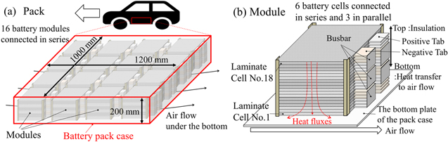
Figure 1. Overview of (a) the target battery pack, and (b) a battery module. Note that such a battery pack does not actually exist and is only a design assumed for this modeling.
Download figure:
Standard image High-resolution imageTable I. Performance of the targeted battery pack. Note that such a battery pack does not actually exist and is only a design assumed for this modeling.
| Type | Items | Spec |
|---|---|---|
| Pack | Assumed size | 1200 × 1000 × 200 mm |
| Typical power | 61 kWh | |
| Capacity | 172.5 Ah | |
| Operation range | 288.0–403.2 V | |
| Cooling method | Heat transfer to outside air only | |
| Laminate cell | Component | 16 modules connected in series |
| Total: 288 laminate cells | ||
| Size | 260 × 220 × 8 mm | |
| Capacity | 57.5 Ah | |
| Operation range | 3.0–4.2 V | |
| Electrode chemistry | Cathode: Liy (Ni1/3 Co1/3 Mn1/3)O2 /Anode: Lix C6 | |
| Number of sheets | Cathode: 31/Anode: 32 | |
| Electrolyte chemistry | LiPF6 EC: DEC = 1:1 vol % |
Single particle model
Most system simulations adopt models based on electrical ECMs as battery models because they have low calculation costs. Meanwhile, models based on electrochemical phenomena, such as the Newman pseudo two-dimensional model, 16,22 have the advantage of being faithful to the electrochemical mechanism, which makes the understanding of the results obvious. In particular, they are used for cyclic degradation and internal short circuits. In the proposed model, the single particle (SP) model 23 is adopted for each cell. This model can reproduce electrochemical phenomena with a relatively low computational cost.
During the charge/discharge process in a Li-ion battery, Li ions are transported from the positive/negative electrode to the opposite electrode through interfacial reactions on the active materials and diffusion and migration in the electrolyte. Moreover, electrochemical reactions occur at the interface of the active material in the positive/negative electrode. In the SP model, the processes are formulated as a diffusion equation and electrochemical equations, as presented in Table II. Note that these equations are adopted from a previous report 23 and are not developed in this study. The model assumes that the effects of diffusion and migration in the electrolyte are negligible.
Table II. Governing equations of the single particle model. 23 Subscript j indicates a positive or negative electrode. Note that these equations are adopted from a previous report 23 and are not developed in this study.
| Items | Equations |
|---|---|
| Active material |
 [1] [1] |
| Active material/electrolyte interface |
 [2] [2] |
 [3] [3] | |
 [4] [4] | |
 [5] [5] |
From the electric current conservation law in each battery cell, the relationship between the current applied to the battery cell  and the current density on the active material interface
  is described by the following equation:

where  is the total interface area of the active materials, and subscript j indicates the positive or negative electrode.
  has opposite signs for the positive and negative electrodes.
  has a positive charge value and a negative value on discharge.
  is calculated using the following equations:

where  is the volume of the active material in each cell,
  is the specific area of the active material,
  is the area of the electrode sheet,
  is the thickness of the electrode sheet,
  is the volume fraction of the active material, and
  is the radius of the active material particle.
The input parameters of the model are presented in Table III. These values are the same as those of our prototype cell reported in a previous study, 17 although the area of the sheet is adjusted to match the capacity of 57.5 Ah. The parameters were also validated with the actual discharge curve of the alternating current impedance in a state of charge (SOC) of 100 %, 17 and it was confirmed that these values were similar to those reported in other studies. 23 In detail, the capacity is defined as the amount of electrons applied to the battery in order for the open-circuit voltage (OCV) to be between 3.0V and 4.2V, and this value is 57.5Ah per cell. Since OCV assumes no dependence on temperature in this study, the capacity does not change with temperature. In addition, the improvement of Li diffusivity at high temperatures is taken into account shown in Table III, and the decrease in internal resistance is taken into account.
Table III. Input parameters for the single particle model. 17 T indicates the temperature.
| Item | Parameter | Unit | Value |
|---|---|---|---|
| Positive electrode | Thickness 
| μm | 42 |
Volume fraction of the active material 
| — | 0.29 | |
Particle radius 
| μm | 4.85 | |
Diffusion coefficient 
| m2s−1 | 2.2 × 10⁻¹² exp(−9.2 × 10²/T) | |
Rate coefficient 
| m2.5mol−0.5 s−1 | 1.8 × 10⁻⁸ exp(−1.1 × 10³/T) | |
| Negative electrode | Thickness 
| μm | 55 |
Volume fraction of the active material 
| — | 0.39 | |
Particle diameter 
| μm | 13 | |
Diffusion coefficient 
| m2s−1 | 9.9 × 10⁻¹² exp(−1.6 × 10³/T) | |
Rate coefficient 
| m2.5mol−0.5 s−1 | 1.5 × 10⁻⁸ exp(−1.6 × 10³/T) | |
| Common | Area of the electrode sheet 
| m2 | 3.55 |
The assumptions made for the model are as follows.
- (1)The Li concentration in the active material in the cell is described as the concentration of two representative particles.
- (2)The impact of the electrolyte and current-collecting foil is negligible.
Cycle degradation model
The capacity of a Li-ion battery decreases and its internal resistance increases with repeated charging and discharging, which is known as cyclic degradation. In each cell, the proposed model considers the impact of the solid electrolyte interface (SEI) layer growth in negative electrodes, phase transition in positive electrodes, and crack propagation. These models were proposed in a previous study. 17 Table IV lists the governing equations. Note that these equations are adopted from a previous report 17 and are not developed in this study.
Table IV. Governing equations of the cycle degradation model. 17 Note that these equations are adopted from a previous report 17 and are not developed in this study.
| Items | Equations |
|---|---|
| SEI layer growth in negative electrodes |
 [8] [8] |
 [9] [9] | |
 [10] [10] | |
 [11] [11] | |
| Phase transition in positive electrodes |
 [12] [12] |
 [13] [13] | |
| Crack propagating |
 [14] [14] |
 [15] [15] |
As shown in Equation 15 in Table IV, in this model the crack propagation is assumed to be dependent on the total transported electric charge amount  It is calculated by integrating the applied current to the battery cell. Therefore, in this model it is assumed that cracks in the cell are always generated by the application of current, and note that crack propagation is not predicted by stress evaluation. Furthermore, the resistance due to cracks is not estimated from the size of a single crack, but represents the frequency of occurrence of multiple cracks that resist the current flowing in the active material. It is assumed that there are no cracks in the initial state, and that if the current is sufficiently advanced, the resistance will be extremely high due to the numerous cracks. However, because of Equation 14 in Table IV, it is necessary to provide initial resistance due to cracking, and the value should be small enough to have no effect.
Owing to the SEI layer growth, the capacity loss of the negative electrode is taken into account by the following equation:

where  is the Li-ion concentration modified for the capacity loss,
  is the Li concentration, and
  is the capacity loss. In the SP model,
  was used instead of
  The variation in the overpotential of the main reactions due to SEI is described by the following equation:

where  is the overpotential,
  is the open-circuit potential,
  is the thickness of the SEI, and
  is the electric conductivity of the SEI layer. The subscript n indicates the negative electrode.
The variation in overpotential due to the phase transition in positive electrodes is described by the following equation:

where  is the resistance per unit cross-sectional area owing to phase transition. The subscript p indicates a positive electrode.
The voltage of each cell  is calculated by the following equations:
where  is the difference in the electrical potential between the active materials and the electrolyte, and
  is the resistance due to crack propagation. In this model, crack propagation considers the impact of the cell as a whole cell, rather than the impact of the positive and negative electrodes individually.
  has a positive charge value and a negative value on discharge. The
  in each cell is adjusted so that the cell voltage
  is the same among the three cells connected in parallel.
Heat generation  is calculated by the following equation:

The input parameters of the model are listed in Table V. These values are the same as those of our prototype cell reported in a previous study 17 and were determined using cycle degradation test data at 25 °C and 70 °C.
Table V. Input parameters for the cycle degradation model. 17 T indicates the temperature.
| Item | Parameter | Unit | Value |
|---|---|---|---|
| SEI growth in negative electrodes | Initial overpotential 
| V | 0.3 |
Exchange current density 
| A m−2 | 5.4 × 10¹¹ exp(−7.6 × 10³/T) | |
Molar weight of SEI 
| kg mol−1 | 0.01 | |
Density of SEI 
| kg m−3 | 1000 | |
Conductivity of SEI 
| S m−1 | 3.41 | |
| Phase transition in positive electrodes | Cover rate 
| s−1 | 1.8 × 10¹⁰ exp(−1.0 × 10⁴/T) |
Resistance per unit cross-sectional area 
| Ω m2 | 0.1 | |
| Crack propagating | Initial resistance 
| Ω | 1.0 × 10⁻⁴ |
Constant 
| s−1 | 7.6 × 10⁻⁵ |
The assumptions made for the model are as follows.
- (1)The side reactions that cause SEI occur uniformly throughout the negative active material in the cell.
- (2)The capacity shift occurs only at the negative electrode.
- (3)The phase transition that causes an increase in internal resistance occurs uniformly throughout the positive active material in the cell.
- (4)The crack propagation that causes an increase in internal resistance occurs uniformly throughout the cell.
Electrochemical–thermal coupled model
The thermal ECM is adopted for modeling the thermal phenomena in the battery pack, as in most system simulations. In this model, the thermal resistance, heat capacity, and heat generation are linked. The temperature of each component is calculated using the energy-balance equation.

where CT is the heat capacity of a cell and is calculated using the following equation:

where  is the cell density,
  is the cell volume equal to 4.6 × 10⁻⁴ m3, and
  is the cell-specific heat at a constant pressure. Qlink
is the heat transfer into or from the linked components, which can be determined from the following equation:
is the cell-specific heat at a constant pressure. Qlink
is the heat transfer into or from the linked components, which can be determined from the following equation:

where  is the temperature difference between the targeted component and the linked components, and RT
is the thermal resistance of a cell, calculated by the following equation:
is the temperature difference between the targeted component and the linked components, and RT
is the thermal resistance of a cell, calculated by the following equation:

where  is the cell thickness equal to 8.0 mm,
  is the cell width equal to 260 mm,
  is the cell depth equal to 220 mm, and
  is the cell thermal conductivity in the thickness direction.
The thermal resistance between the pack case and the outside air RT,ht , is described by the following equation:

where h is the heat transfer coefficient and  is the cross-sectional area of the air. The heat transfer coefficient under turbulence flow can be calculated by the following equation:
24
is the cross-sectional area of the air. The heat transfer coefficient under turbulence flow can be calculated by the following equation:
24

where Nu is the Nusselt number, L is the width of the case,  is the thermal conductivity of air, Re is the Reynolds number, and Pr is the Prandtl number. For the sake of simplicity,
  does not take into account the time dependence and is calculated from the average speed of the BEV.
A schematic of the electrochemical–thermal coupled model for the battery pack is shown in Fig. 2. Each module is connected with the bottom of the pack case whose thermal resistance is negligible. Note that the modules are not connected to the rest of the case and are insulated. This is because this battery pack is mounted on the bottom of the car as shown in Fig. 1a, and is assumed to be in contact with the car's parts intricately in all areas except the bottom. In reality, there is some heat conduction passes between the parts in contact with each other, but for the sake of simplicity, this is not taken into account and is assumed to be insulation. In each cell, the electrochemical models and the thermal ECMs are coupled for temperature and heat generation. The model is constructed by using MATLAB Simulink® R2020a/Simscape. The input parameters of the model are listed in Table VI. Furthermore, the time step was fixed at 1.0 s. This was not the minimum time for convergence, but was set to sufficiently account for the time variation of the heat generation.
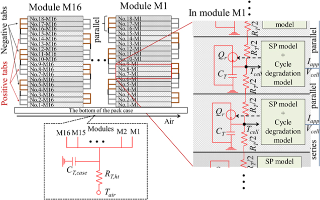
Figure 2. Schematic of the electrochemical–thermal coupled model for the battery pack. The red lines indicate the thermal connections, and the blue lines indicate the electrical connections.
Download figure:
Standard image High-resolution imageTable VI. Input parameters for the thermal equivalent circuit model.
| Parameter | Unit | Value |
|---|---|---|
Cell density 
| kg m−3 | 2003 20 |
Cell specific heat 
| J kg−1K−1 | 793 20 |
Cell thermal conductivity in the thickness direction 
| W m−1K−1 | 1 20 |
Heat capacity of the pack case 
| J K−1 | 9.05 × 10⁴a) |
| Average Reynold number of air Re | — | 7.22 × 10⁵b) |
| Prandtl number of air Pr | — | 0.717 25 |
Heat transfer coefficient 
| W m−2K−1 | 40.5 b) |
a): Assumed value. b): Calculated with the average speed of the worldwide-harmonized light vehicles test cycles (WLTC) class 3b. 26,27
The assumptions made for the model are as follows.
- (1)The heat transfer in the direction perpendicular to the cell stacking is negligible.
- (2)The thermal capacity of things, except the cell and case, is negligible.
- (3)The heat is dissipated only to the outside air at the bottom of the case and is insulated from the rest.
- (4)The temperature at the center of the cell is representative of the electrochemical phenomena of the whole cell.
- (5)The heat transfer coefficient to the outside air can be estimated as the average of the driving speed of the BEV.
Internal short circuit model
According to the statistics of EV fire incidents of electric vehicles between 2014 and 2019, internal short circuits (ISCs) accounted for 52% of the accident probability. 28 Therefore, more accurate predictions of ISCs and the development of battery management systems based on them could be invaluable in designing safer battery packs. The main causes of ISCs are mechanical damage, 29 manufacturing defects, 30,31 overcharge, 32 and overdischarge. 33,34 ISCs are expected to develop gradually. The early stages of ISCs, such as shorts of 100/10/1 Ω, have remaining time for them to run into thermal accidents because of their low heat generation power. 35 Finally, the resistance of ISCs might become sufficiently small to lead to thermal runaway. In the proposed model, the early stage of ISCs in a cell is modeled to predict the impact of electrochemical and thermal phenomena in the battery pack.
Because the phenomena in an ISC cell are three-dimensionally complicated, it is not appropriate to use ECMs to predict them. Therefore, only the ISC cell is considered a three-dimensional phenomenon by using the finite element method. A schematic of the ISC cell model is shown in Fig. 3. This model is based on the ECM and includes the 3D detailed model of the ISC cell. In this model, the short-circuit object (SCO) is assumed to be in the center position of the cell. In the case of internal short-circuit phenomena, the resistance differs depending on the connection scenario between the Al/Cu foil and positive/negative electrode. 18 The early stage of ISCs is not assumed to be the scenario of the connection between the Al foil and Cu foil because it has the lowest resistance and is considered to be at risk of thermal runaway. Nevertheless, for the sake of simplicity, the early stage of ISCs is reproduced by adjusting the resistance of the SCO, and the scenario of the connection between the foils is assumed in the model shown in Fig. 3b. Moreover, as shown in Fig. 3c, the ISC cell is assumed to be in position 18. This is because the temperature is the highest in this cell, and the situation is prone to ISCs. Based on previous reports,18,29 the shape of the SCO is modeled as a cylinder with a diameter of 3 mm.
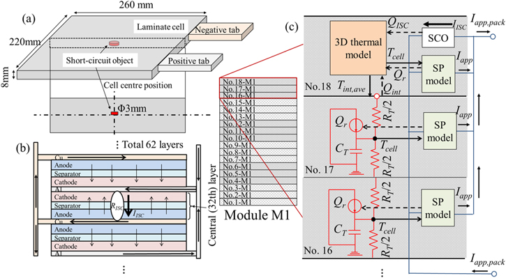
Figure 3. (a) Position of the short-circuit object, (b) current flow path in the internal short circuit cell, and (c) schematic of the connection between the internal short circuit cell and other cells.
Download figure:
Standard image High-resolution imageThe ISC cell model was constructed based on the nail penetration model proposed by us in a previous report.
20
The electric current through the SCO  is described by the following equation:

where  is the difference in the electric potential between the Al and Cu foils, and
  is the resistance of the SCO. In this model, assuming that the electrical resistance of the current collector foil and tabs is negligible,
  is calculated using the following equation:

The above equations, the SP model, and the cycle degradation model are coupled to calculate the electrochemical state of the ISC cell and two parallel-connected cells, as shown in Fig. 3c. The heat generation of the SCO QISC is described by the following equation:

The thermal phenomena in the ISC cell are presented as a heat transfer equation, which is described by the following equation:

where  is the thermal conductivity vector, and
  is the heat generation density. The volume integral of
  is
is  in the electrode domain, and
  in the SCO domain. The input parameters in the above equation are the same as those listed in Table VI. As shown in Fig. 3c, the thermal connection on the interface between the ISC cell and the adjacent cell is taken into account by exchanging the heat
  and the average temperature
  In other words, the 3D detailed model of the ISC cell and the ECM of the other cells are solved simultaneously, taking into account the connections. The ISC cell model was constructed using COMSOL Multiphysics® 5.6, and the electric–thermal connection was achieved by LiveLink for Simulink.
The calculation meshes of the ISC cell model are shown in Fig. 4. The prism meshes were adopted, and the total number of elements was 42,850. It is confirmed that the calculation results do not vary with more refined meshes. For the same reason, the relative tolerance of the progress for the next time step was set as 1.0 × 10⁻³. This model adopted the backward differentiation formula in COMSOL Multiphysics® and the time step is automatically determined for each step. When the calculation of the thermal ECM advances one step, the data of temperature and heat generations are exchanged if the calculation of above ISC model advances to the same time.
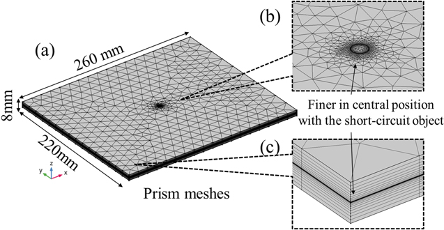
Figure 4. Overview of the calculational meshes. (a) General overview and (b), (c) engaged overviews.
Download figure:
Standard image High-resolution imageThe assumptions made for the model are as follows.
- (1)The impact of the current in the current-collecting foils and tabs is negligible because of the lower current flow under the early stage ISCs.
- (2)The current passing through the SCO is not limited to the discharge of the ISC cell, but also includes the discharges of two cells connected in parallel.
- (3)The scenario of the connection between the foils was assumed in the model, and the resistance of the SCO was adjusted to reproduce the early stage ISCs.
- (4)The ISC cell is assumed to be in position No. 18, as shown in Fig. 3c, because the temperature is the highest in this cell and the situation is prone to ISCs.
Validation of the proposed models
In this study, the proposed model for the battery pack was not validated based on experimental methods. Battery packs are of the scale actually installed in BEVs, and it is estimated that the experimental measurement of these packs will require a significant effort in terms of equipment. We recognize that this type of validation with experimental approaches is extremely important and should be carried out. Nevertheless, in this study, we focus only on modeling, and this validation remains as future work.
Despite of the above fact, at the cell level, each model that constitutes the proposed model has been validated using the experimental methods reported in previous studies. 17,20 All input parameters of the proposed model were set based on the prototype cell. The results of the SP model were confirmed to be in good agreement with those of the actual discharge curve and the alternating current impedance in the state of charge (SOC) 100%. 17 Moreover, the results of the cooperation between the SP model and the cycle degradation model were confirmed to be in good agreement with those of cycle degradation tests at 25 °C and 70 °C. 17 Finally, the ISC cell model is based on the nail penetration model, and the results of the temperature variation on the cell surface were confirmed to be in good agreement with those of the actual nail penetration tests. 20 Therefore, if the scale effects are negligible, the proposed model for the battery pack may be considered a reasonable model.
Estimation of electrical power applied for battery pack in operation
The electrical power applied to the battery pack is estimated by the electric consumption model for BEVs published by the Environmental Partnership Council (Tokyo, Japan, https://epc.or.jp/sim_2019model_english, accessed on, December 12/29/2020). In this model, the systems that make up the BEV, such as the vehicle mechanism, motor, and direct current (DC)-DC converter, are built in MATLAB Simulink®. The system simulation was similar to that in several reports. 36 As this study focuses on the battery pack system, the features are not presented.
The typical input parameters for the BEV system simulation are listed in Table VII. In this condition, the calculation results of the electrical power are shown in Fig. 5. These are the electrical power required for the BEV to run at the speed pattern of the worldwide-harmonized light vehicles test cycles (WLTC) class 3b, 26,27 shown in Fig. 5. Note that positive values of the electrical power indicate the charge, and a negative value indicates the discharge. In this model, regenerative braking is considered, and charging occurs when the vehicle stops.
Table VII. Typical input parameters for the BEV system simulation.
| Item | Unit | Value |
|---|---|---|
| Speed pattern | m s−1 | The worldwide-harmonized light vehicles test cycles (WLTC) class 3b, 26,27 shown in Fig. 5 |
| Total weight of the vehicle | kg | 1481 36 |
| Cabin volume | m3 | 3.28 36 |
| Setting temperature | ||
| in the cabin | °C | 20 a) |
| Motor efficiency | — | 0.89 36 |

Figure 5. Speed pattern of WLTC class 3b and calculation results of the variation of the electrical power applied for the battery pack. Note that positive values of the electrical power indicate the charge and negative values indicate the discharge.
Download figure:
Standard image High-resolution imageAs the electrical power is equal to the values in Fig. 5, the electric current applied to the battery pack  is calculated by the following equation:

where  is the electrical power, and
  is the voltage of the battery pack.
Results and Discussion
Standard condition
As the standard condition, the calculation is performed as follows:
- (1)The environmental and initial temperatures were 20 °C.
- (2)The initial Li concentrations in all the cells were set as values corresponding to SOC = 100%.
- (3)Initially, all cells were completely free of cycle degradation.
- (4)The power pattern shown in Fig. 5 was applied repeatedly until the calculation was stopped.
- (5)The calculation stops when the battery pack voltage reaches the lower limit of 288 V.
The calculation time for this simulation was 1.7 h using a general computer (CPUs:Intel® Xeon® Gold 6130 CPU@2.10GHz, Memory size:128 GB). The calculation results are presented in Fig. 6. Under this condition, the temperature results for module M1 are shown as representative because all the modules are in the same state. The applied current varied between approximately ±100 A. The voltage of the entire battery pack decreases slowly over time with a variation of approximately ±5 V until it reaches 288 V in 9.34 h. If the operation time is converted into driving distance, it is equivalent to 430 km. This is a large value considering that the driving ranges of the popular EVs released in 2017 or 2018 were 220–430 km. 37 However, 430 km may be a normal BEV specification in 2021 because the range has increased significantly in recent years. For example, the range of the Tesla Model S is estimated to be 647 km.

Figure 6. Under the standard condition, time histories of the applied electric current and pack voltage (a) throughout the entire time and (b) after 9 h, and time histories of temperature of (c) cells No. 1–9 and (d) cells No. 10–18 in a module. Note that all the modules (M1–16) are assumed to be in the same state under these conditions.
Download figure:
Standard image High-resolution imageAs shown in Figs. 6c and 6d, it was confirmed that the temperature in all the cells increased during driving. Cell No. 18 was the farthest from the outside air, and thus the temperature rise was the largest. At the final time, the temperature of No. 1 is 20.7 °C, that of No. 18 is 22.2 °C, and the average value is 21.7 °C. Note that this calculation model does not consider the contact thermal resistance, and thus the temperature may be lower than the actual value.
Impact of the SCO electric resistance
Assuming that cell No. 18 of module M1 is the state of the ISCs, the calculations are performed under three conditions: the SCO electric resistance is 100 Ω, 10 Ω, or 5 Ω. The resistance values are in the early stages of ISC. 35 The other conditions were the same as those in the standard condition. The results of the time histories are presented in Fig. 7. From Fig. 7b, at stop time the voltages of module M1 are 54.02 V (standard condition), 53.96 V (100 Ω), 53.20 V (10 Ω) and 51.52 V (5 Ω). These differences are due to self-discharge and are very small for the pack voltage, as shown in Fig. 7a. Therefore, there was no significant difference in the driving ranges presented in Table VIII.
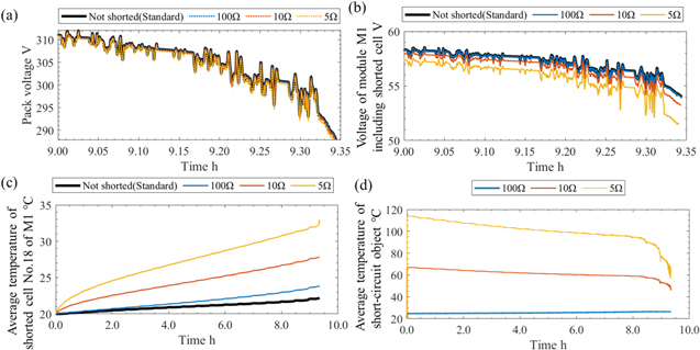
Figure 7. Time histories of (a) the pack voltage, (b) the voltage of module M1 including shorted cell No. 18, (c) the average temperature of shorted cell No. 18 of module M1, and (d) the average temperature of the short-circuit object. Note that the time range of (a), (b) is from 9 h to the stop time.
Download figure:
Standard image High-resolution imageTable VIII. Impact of ISCs for driving ranges.
| Item | Not shorted (Standard) | 100 Ω | 10 Ω | 5 Ω |
|---|---|---|---|---|
| Driving range km | 430.0 | 430.0 | 429.9 | 429.7 |
From Fig. 7c, average temperature of the shorted cell No. 18 increases during driving and at stop time it reaches 23.9 °C (100 Ω), 27.9 °C (10 Ω), and 33.0 °C (5 Ω). This may be due to the fact that the smaller the short-circuit resistance is, the greater the amount of current carried and the greater the amount of heat generation. As shown in Fig. 7d, the average temperature of the SCO increases immediately after the driving starts and decreases slowly until the stop time. The temperature reaches a maximum of 26.5 °C (100 Ω), 67.1 °C (10 Ω), and 114.2 °C (5 Ω). As the maximum temperature in the case of 5 Ω reaches 90 °C, where the SEI layer begins to decompose and self-heating is initiated, 38 the risk of thermal runaway is high. The SCO resistance, which is the limit of thermal runaway, was considered to be between 5 and 10 Ω. Figure 8 shows the temperature distribution in the shorted cell (No. 18) at the stop time in the case of 5 Ω. The high temperature is near the short-circuit (within a few millimeters), and the distribution is relatively uniform in most of the cells. From the voltage results, it can be observed that an ISC in one cell has only a very small effect on the battery pack voltage as a whole. Nevertheless, the temperature in the vicinity of the SCO is very high, and if thermal runaway occurs, it could lead to a major accident. Therefore, the battery management system, including the detection of internal shorts, must be sufficiently accurate.
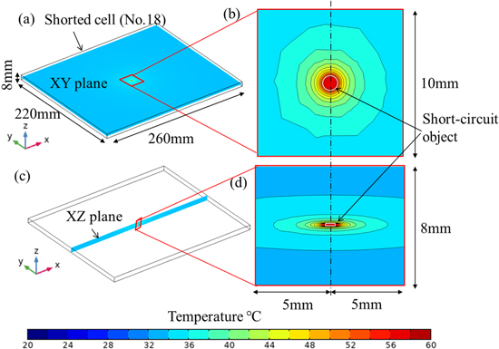
Figure 8. In the shorted cell (No. 18), temperature distributions on (a) XY plane and (c) XZ plane at the center of the short-circuit object at the stop time in the case of 5 Ω; (b) is the enlarged view of (a), and (d) is the enlarged view of (c).
Download figure:
Standard image High-resolution imageThe results for each cell in the modules at the stop time are shown in Fig. 9. Note that module M1 includes the shorted cell, M2–16 are not shorted, and M2–16 are assumed to be in the same state under these conditions. As shown in Fig. 9a, the temperature in module M1 varies approximately linearly from No. 1 to No. 18 in the cases of ISCs, and the larger the cell number is, the larger the temperature difference compared to the non-shorted case (standard condition). The average temperature rise of No. 18 in module M1 is 2.2 °C (not shorted), 3.9 °C (100 Ω), 7.9 °C (10 Ω), and 13.0 °C (5 Ω), and in the case of 5 Ω, the temperature rise is 6 times higher than that of the not shorted case.
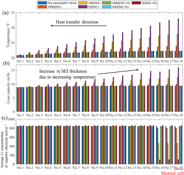
Figure 9. Results of each cell in modules at the stop time for each internal short circuit resistance: (a) shows temperature, (b) shows loss capacities, and (c) shows average Li concentration of the negative electrode. Note that module M1 includes the shorted cell, M2–16 are not shorted, and M2–16 are assumed to be in the same state under these conditions.
Download figure:
Standard image High-resolution imageFrom Fig. 9b, it can be observed that the capacity loss during driving increases with a larger number. This is because the SEI layer thickness increases with increasing temperature. The loss capacity of No. 18 in module M1 is 9.3 mAh (standard condition), 9.9 mAh (100 Ω), 12.5 mAh (10 Ω), and 15.9 mAh (5 Ω), and in the case of 5 Ω, the loss capacity is 1.7 times higher than that of the standard condition. As the capacity difference becomes more pronounced with repeated driving, over-discharge is likely to occur. Over-discharge is considered to be one of the factors of ISCs, 33,34 and if the frequency of this incident increases, the ISC stage may develop.
From Fig. 9c, it can be observed that the Li concentration of the negative electrode at cells No. 16–18 in module M1 is lower than that of the other cells, and it is almost exhausted in the case of 5 Ω. This is because these three cells are connected in parallel and are significantly affected by discharge to the ISCs. Therefore, these cells are prone to over-discharge, which induces ISCs. Thus, it can be observed that an ISC increases the risk of thermal runaway not only in the cell where it occurs, but also in parallel-connected cells.
Impact of number of runs
Using the standard condition as a basis, numerical simulations are performed in which the driving from SOC = 100% to the stop condition is repeated 1000 times. It is assumed that there are no cells in which ISCs occur. The state of cycle degradation at the last time in the run was set as the initial state of the next run. The Li concentration was set as SOC = 100% in the initial state, and the effect of charging from SOC at the stop time to SOC = 100% is not considered.
In this part, comparisons of the internal resistance of each cell is shown. The internal resistance is defined in the following equations:

where  is the internal resistance per cell. Since this parameter is time varying, the time average from the start time to 0.5 h, when the first speed pattern of WLTC class 3b of each cycle, is used for comparison.
Figure 10 shows the time histories of the pack voltage for driving at the 1st, 400th, 700th, and 1000th run. From the start of the driving up to 6 h, the behavior was almost the same. After 6 h, the larger the number of runs is, the larger the voltage drop. This is due to the increase in the SEI film and the internal resistance caused by cyclic degradation. As presented in Table IX, the driving range also decreases with the number of runs, and the range of the 1000th run is 15 % lower than that of the standard condition.
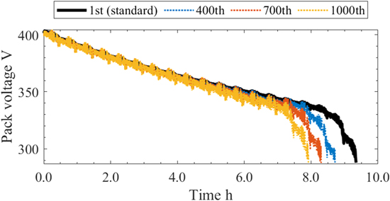
Figure 10. Time histories of the pack voltage for each number of runs.
Download figure:
Standard image High-resolution imageTable IX. Impact of number of runs for driving ranges.
| Item | 1st (Standard) | 400th | 700th | 1000th |
|---|---|---|---|---|
| Driving range km | 430.0 | 400.3 | 380.6 | 364.4 |
Figure 11 shows the results for each cell in a module at the stop time for each number of runs. Note that all modules (M1–16) are assumed to be in the same state under these conditions. As shown in Fig. 11a, the larger the number of runs is, the larger the temperature difference. This is because of the increase in heat generation due to the increase in the internal resistance. The temperature difference of cell No. 18 from the initial state is 2.2 °C (1st run), 5.7 °C (400th), 6.8 °C (700th), and 7.2 °C (1000th), and in the case of the 1000th run, the temperature rise is 3.3 times higher than that of the first run. This large difference in the temperature of the cells in the module is considered to cause a difference in the degradation degree, which reduces the overall performance of the module.

Figure 11. Results of each cell in a module at the stop time for each number of runs: (a) shows temperature, (b) shows accumulated loss capacities, and (c) shows internal resistance averaged from the start time to 0.5 h. Note that all the modules (M1–16) are assumed to be in the same state under these conditions.
Download figure:
Standard image High-resolution imageAs shown in Fig. 11b, the larger the number of runs, the larger the loss capacities accumulated from the first run. The accumulated loss capacity of cell No. 18 is 3.8 Ah (400th run), 6.5 Ah (700th), and 9.0 Ah (1000th), and in the case of the 1000th run the capacity is 16 % lower than the initial capacity 57.5 Ah. Moreover, the difference in the accumulated loss capacitance between cells No. 1 and No. 18 is 0.37 (400th run), 0.74 (700th), and 1.10 Ah (1000th), and it increases owing to the increase in the number of runs.
As shown in Fig. 11c, the larger the number of runs is, the larger the internal resistance averaged from the start time to 0.5 h. The internal resistance of cell No. 18 is 0.8 mΩ (1st run), 1.8 mΩ (400th), 2.1 mΩ (700th), and 2.2 mΩ (1000th), and in the case of the 1000th run, the internal resistance is 2.8 times higher than that of the first run.
Impact of environmental temperature
Using the driving conditions in the previous section as a basis, numerical simulations were performed when the environmental temperature and the initial temperature of the cells were set as 30 °C or 40 °C.
Figure 12 shows the time histories of the pack voltage for each environmental temperature. In the first run, there was almost no difference in voltage, but in the 300th run, the difference became larger, especially at the end of the run. This is because the degree of cycle degradation is more advanced at higher temperatures. As presented in Table X, in the first run, the driving range increases slightly with the environmental temperature because of the increase in the electrochemical reaction characteristics, which induces a decrease in the internal resistance. In this calculation, the electric power applied to the battery was assumed to be 20 °C. Therefore, note that the driving range is assumed to be larger than in the actual condition owing to differences in air conditioning settings. At the 300th run, the driving range decreases with the environmental temperature because of the decrease in the capacity and increase in the internal resistance. The range at 40 °C in the 300th run was 17 % lower than that in the first run. The loss of the driving range is 3.5 times larger than that at 20 °C, which indicates that the cycle degradation progresses approximately 3.5 times faster.

Figure 12. Time histories of pack voltage for each environmental temperature at (a) the first run and (b) the 300th run.
Download figure:
Standard image High-resolution imageTable X. Impact of environmental temperature for driving ranges. Unit: km.
| Number of runs | 20 °C | 30 °C | 40 °C |
|---|---|---|---|
| 1st | 430.0 | 430.1 | 430.8 |
| 300th | 408.8 | 385.5 | 355.9 |
Figure 13 shows the results for each cell in a module at the stop time for each environmental temperature. Note that all the modules (M1–16) are assumed to be in the same state under these conditions. As shown in Fig. 13a, in the first run, the larger the environmental temperature is, the smaller the temperature difference. This is because of the decrease in the internal resistance due to the temperature increase. Nevertheless, at the 300th run, this trend was reversed owing to the effects of cycle degradation.
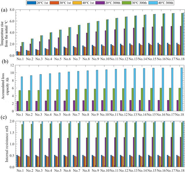
Figure 13. Results of each cell in a module at the stop time for each environmental temperature: (a) shows the temperature rise from the initial condition, (b) shows accumulated loss capacities, and (c) shows internal resistance averaged from the start time to 0.5 h. Note that all the modules (M1–16) are assumed to be in the same state under these conditions.
Download figure:
Standard image High-resolution image
As shown in Fig. 13b, the higher the environmental temperature is, the larger the loss capacities accumulated from the first run. The accumulated loss capacity of No. 18 at the 300th run is 2.8 Ah (20 °C), 6.0 Ah (30 °C), and 11.3 Ah (40 °C), and in the case of 40 °C, the capacity is 20 % lower than the initial capacity of 57.5 Ah.
From Fig. 13c, the trend of the internal resistance is as described above. At the 300th run, the internal resistance of cell No. 18 was 1.3 mΩ (20 °C), 1.9 mΩ (30 °C), and 2.0 mΩ (40 °C), and in the case of 40 °C, the internal resistance was 4.4 times higher than that of the first run. Thus, it can be confirmed that the environmental temperature has a significant effect on capacity loss and internal short circuits.
Conclusions
In this study, we proposed an electrochemical–thermal coupled model to predict phenomena in battery packs while driving BEVs. The model considers the cycle degradation and ISCs per single cell in the battery pack. The quantitative evaluations have been performed focused on the three impacts of (i) the SCO electric resistance, (ii) number of runs, and (iii) environmental temperature.
Regarding the impact of the SCO electric resistance, there is no significant difference in the driving ranges in the first run. In the case of 5 Ω, at the end of the run, the temperature rise is 6.0 times higher and the loss capacity is 1.7 times higher than those in the standard condition. Moreover, from the SCO temperature, it is confirmed that the risk of thermal runaway in the case of 5 Ω is high. In the shorted cell and parallel-connected cells, the Li concentration of the negative electrodes is almost exhausted at the end of the run. Therefore, these cells are prone to over-discharge, which induces ISCs.
Concerning the impact of the number of runs, the driving range decreases with the number of runs, and the driving range of the 1000th run is 15 % lower than that of the first run. In the case of the 1000th run, at the end of the run, the accumulated loss capacity of cell No. 18 is 16 % lower than the initial capacity of 57.5 Ah, and the internal resistance is 2.8 times higher than that of the first run.
With respect to the impact of environmental temperature, at the 300th run, the driving range decreases with the environmental temperature because of the decrease in the capacity and increase in the internal resistance. The driving range at 40 °C in the 300th run is 17 % lower than that in the first run. The loss of the driving range is 3.5 times larger than that at 20 °C, which indicates that the cycle degradation progresses approximately 3.5 times faster. In the case of 40 °C, at the end of the run, the accumulated capacity of cell No. 18 is 20 % lower than the initial capacity of 57.5 Ah, and the internal resistance is 4.4 times higher than that of the first run.