
Abstract
Presented here, is an extensive 35 parameter experimental data set of a cylindrical 21700 commercial cell (LGM50), for an electrochemical pseudo-two-dimensional (P2D) model. The experimental methodologies for tear-down and subsequent chemical, physical, electrochemical kinetics and thermodynamic analysis, and their accuracy and validity are discussed. Chemical analysis of the LGM50 cell shows that it is comprised of a NMC 811 positive electrode and bi-component Graphite-SiOx negative electrode. The thermodynamic open circuit voltages (OCV) and lithium stoichiometry in the electrode are obtained using galvanostatic intermittent titration technique (GITT) in half cell and three-electrode full cell configurations. The activation energy and exchange current coefficient through electrochemical impedance spectroscopy (EIS) measurements. Apparent diffusion coefficients are estimated using the Sand equation on the voltage transient during the current pulse; an expansion factor was applied to the bi-component negative electrode data to reflect the average change in effective surface area during lithiation. The 35 parameters are applied within a P2D model to show the fit to experimental validation LGM50 cell discharge and relaxation voltage profiles at room temperature. The accuracy and validity of the processes and the techniques in the determination of these parameters are discussed, including opportunities for further modelling and data analysis improvements.
Export citation and abstract BibTeX RIS

This is an open access article distributed under the terms of the Creative Commons Attribution Non-Commercial No Derivatives 4.0 License (CC BY-NC-ND, http://creativecommons.org/licenses/by-nc-nd/4.0/), which permits non-commercial reuse, distribution, and reproduction in any medium, provided the original work is not changed in any way and is properly cited. For permission for commercial reuse, please email: oa@electrochem.org.
The electrification of the transport and energy sectors has been aided by the falling cost of lithium-ion batteries over the past several years.1–3 As demand for lithium-ion batteries soars, the requirements imposed by the commercial sector have become more stringent. The development of batteries that are safer, longer-lived, more energy dense, more power dense, and cheaper has required a concerted research effort from multiple disciplines. For many years this research had focused on improvements in the chemistry, but more recently incremental gains in battery performance have been realized by reengineering of the manufacturing processes and innovation in the models that help us to understand battery performance during their operation.
Battery models describing the behavior of the battery are a useful tool to design and manage batteries in a more efficient way. There are various approaches to battery modelling depending on the complexity and resolution required. These models can typically be classified into two different families: equivalent circuit models4–7 and physics-based models.8–10 Physics-based models rely on physical laws to describe the electrochemistry inside of the battery and hence offer a better understanding of the underlying physics. These models are computationally expensive and require many parameters, however they provide detailed insight in the different electrochemical phenomena involved in the performance of the battery. In addition, the parameters have a clear physical relevance but need to be measured or determined by performing a range of experiments, which is a challenge. Another benefit of these physics-based models is that they can be coupled to other physics-based models in a consistent way, in order to extend their capabilities and incorporate other physical phenomena, such as thermal11–13 or degradation effects.14,15
The most widely used physics-based lithium-ion battery model was introduced by Newman and his collaborators to describe the behavior of a porous electrode battery.8–10,16 This model is commonly known as a pseudo-two-dimensional (P2D) model as it assumes that at each point of the electrode there is a spherical particle which is representative of the active material, so there is one spatial dimension for the electrode thickness and another spatial dimension for the radius of each particle.17,18 This model has been thoroughly studied and has been used as a powerful tool for estimating, optimizing and predicting battery performance. The parameters of the P2D model describe the physical, chemical and electrochemical properties of a cell, therefore the geometric, thermodynamic and kinetic properties of the battery components are all required as inputs.13,19–21 The reliability of the P2D model strongly depends on the accuracy of these parameters, which are specific to each cell design (both in terms of the geometry and the chemistry), so not all the parameter values are transferable from one cell design to another. For this reason, finding a suitable set of parameters to simulate a specific battery is one of the main challenges in battery modelling. One approach is to fit the model to match the experimentally measured voltage. However, given the complexity of the model and the large number of parameters, this approach is often not feasible unless a very good guess of the parameters is provided in advance. In other occasions, parameters from the literature can be used, but if they are taken from different sources inconsistencies might arise leading to poor predictions. Hence, measuring these parameters experimentally is potentially a more robust approach that can lead to more accurate model predictions.
The P2D model requires over 30 parameters to fully describe the physical, chemical, and electrochemical properties of the cell and allow simulation of its behavior, the exact number depending on the way the model is defined. The P2D model used in this investigation requires 35 parameters (Fig. 1, Table VII). Quantifying these parameter values is challenging and time consuming, requiring various characterization and analytical methods. For commercial cell chemistries, this process is even more challenging as manufacturers do not provide parameter, composition or component information in their specification sheets. In the modelling community, parameter sets are often taken from literature, with their origins not necessarily being traced.22 Previous parameterizations have reported studies of both a high energy19,20,23 and a high power cell21 for a physicochemical model, and both cells had a Li(NixMnyCoz)O2 positive electrode and graphite negative electrode. Waldmann et al.24 provided a detailed review of post-mortem techniques for a lithium-ion battery, several of which have been utilised in this investigation. Subsequent electrochemical analysis illustrates the change in cell performance and physico-chemical properties after ageing.14,25,26

Figure 1. Summary of the parameterization requirements and physical, chemical and electrochemical property elucidation.
Download figure:
Standard image High-resolution imageParameterization
In this work we bring together several techniques for the parameterization of a commercial cell P2D model, and we discuss the validity of these approaches. Parameterization is not a simple task, and the process of cell tear down may compromise the cell components. We use a cylindrical LG M50 21700 (LGM50) cell, prior to ageing, to develop these parameterization protocols and tear-down methodologies for extraction of the physical, chemical and electrochemical properties of the cell. We describe the various analytical methods employed to determine information on the geometry, chemistry and electrode microstructure. Particular focus is given to the electrochemical tests of the extracted electrode materials to determine the information on the electrode and cell thermodynamic, kinetics and transport properties. A summary of the required parameters is shown in Fig. 1. The accuracy of the experimental parameters is investigated through comparing the simulations from Python Battery Mathematical Modelling (PyBaMM)27 and experimental validation discharge curves at different currents of the LGM50 cell at room temperature.
We obtain the physical properties of the cells, electrodes and separator from direct measurements after a teardown or cell opening step.28 Porosity and pore domain size are ascertained using several methods; Brunauer–Emmett–Teller (BET) theory is used for fitting gas surface absorption measurements to infer pore sizes of between 3–300 nm. Mercury porosimetry typically measures larger pores, as it is an intrusion technique. This can have limitations in that we observe the "pore neck" rather than full pore size, however larger pore sizes typical for a battery electrode can be measured.29 Porosity in materials and electrodes can be investigated through different imaging techniques such as X-ray tomography30–32 and electron microscopy.33,34 When characterizing the void regions the conductive carbon and binder domain (CBD) should be excluded. CBD is difficult to visualize, especially with graphite or carbon electrodes as the binder and carbon are very similar in their X-ray attenuation.35,36 There has been much work to improve the imaging characteristics of electrode structure, which enables other parameters, such as the tortuosity, the Bruggeman coefficient and the pore shapes, to be estimated and calculated.36 In this work we use focused ion beam milling with scanning electron microscopy (SEM-FIB) to investigate the pore structures of the two electrodes and the separator. This technique gives us quantitative information about the porosity, and also information about the particle shapes and densities, packing density and CBD distribution.37
In terms of the chemical and material properties, the elemental composition of the active materials can be analyzed using inductively coupled plasma optical emission spectroscopy (ICP-OES) and energy-dispersive X-ray spectroscopy (EDS), and X-ray diffraction for the material crystal structure and theoretical density. These are standard techniques utilized as part of teardown and forensics of batteries.28,38 ICP is used for NMC elemental analysis because it can be dissolved in acid. However the negative electrode components SiOx and graphite cannot, therefore the composition is analyzed with EDS only. The exact composition of the NMC is difficult to determine, as it may contain various small quantities of additives such as aluminum or niobium to stabilize the NMC. In addition, aluminum from the current collector must be subtracted from the total, which gives rise to inaccuracies. EDS cannot detect low atomic number elements such as lithium, and care must be taken in obtaining good measurements. Usually flat polished samples are required. Here the EDS measurements are taken from the surface of ion-milled samples in order to obtain good surfaces, reducing the scattering effect, and from top-down images to show the distribution of the elements.
Electrochemical parameterization can be performed by utilizing two-electrode full cells, half cells (with lithium as counter electrode) and three-electrode configurations. All methods have limitations, and therefore a combination is preferred. Two-electrode half cells (with lithium metal counter) enable observation of the working electrode potential (negative electrode or positive electrode). These cells often have higher internal resistances or polarization due to the metal counter electrode, and hence a larger ohmic drop upon cycling is observed.39 Lithium also reacts to form an interface layer on the electrode, which needs to reform upon every redeposition. Therefore the coulombic efficiencies of the half cells are marginally lower than that observed without a lithium metal counter electrode (full cell), which leads to shorter cell lifetimes.40,41 However in the two-electrode half cell configuration the full capacity (or lithiation) of the working electrode can be achieved, as the lithium transfer is not limited by the working electrode. Compared to half cells, full cell testing resembles the operation of a commercial battery more closely. A three-electrode arrangement, is used here, in which the negative and positive electrodes are assembled with a third reference electrode to enable deconvolution of the individual electrode potentials. To operate a stable reference electrode, the cell configuration requires electrochemical and physical symmetry. This is difficult to achieve in a lithium-ion battery configuration where the negative and positive electrodes are different and inherently asymmetric.42 We use a three-electrode configuration with a ring lithium metal reference to elucidate the individual electrode potentials.43 The combination of half cell and full cell three-electrode tests allow analysis of the cell stoichiometry and lithium content within each electrode and in combination provides the fundamental thermodynamic and kinetic parameters for the simulations. The cylindrical LGM50 cell has been utilized to develop these parameterization protocols for the physical, chemical and electrochemical properties.
A range of electrochemical techniques were used to elucidate the thermodynamic and kinetic properties of the materials and electrodes. Galvanostatic intermittent titration technique (GITT) was used to ascertain the open circuit voltage (OCV) of cells in two- and three-electrode configurations, and the diffusion coefficient at different states of charge (SOC).44–46 Cells were also tested using electrochemical impedance spectroscopy (EIS) at different temperatures to calculate the exchange current density for each electrode and their activation energy from the Arrhenius equation, and subsequently the reaction rate was determined.47 The electronic conductivities of the electrodes were measured with a four-point probe. If the composition of the electrode and cell design (negative to positive electrode mass ratio) is already known, this negates the requirement for electrode composition analysis. This means that the capacity loss during formation can be calculated, which determines how much of the lithium from the positive electrode is lost in the first few cycles, and the reversible lithium which intercalates into the graphite. As a result the calculation of stoichiometry and lithium concentration is significantly easier than in a commercial cell. In this work we calculate the concentration from the estimated active material volume, and the stoichiometry is calculated using OCVs measured from the half cells and three-electrode configurations, assuming full lithiation is observed in the two-electrode half cells.
The electrolyte properties, such as the transfer, ionic conductivity and ionic diffusivity were taken from Nyman et al.48 The exact composition of the electrolyte in the LGM50 is unknown, therefore in the electrochemical experiments we utilized a standard electrolyte that was compatible with both electrodes and provided no wettability issues. The electrolyte is 1 mol dm−3 LiPF6 with ethylene carbonate (EC): ethyl methyl carbonate (EMC) (3:7, V:V) which is the same electrolyte studied by Nyman et al., and therefore the parameters determined in that article were utilized in this work.48
Experimental
Cell teardown and physical property analysis
Before teardown of the LGM50 cylindrical cell the cell geometry and dimensions were measured using a Vernier caliper. The cell was discharged to 2.5 V at C/50 (0.1 A) (defined as 0% SOC by the manufacturer) and transferred to an argon glovebox environment for extraction of the electrodes, and best practice was followed for disassembly (<1 ppm of oxygen and water).28
After cell disassembly, pieces of the positive and negative electrodes from the opened cell were soaked in dimethyl carbonate (DMC) overnight to remove electrolyte residue and dried in a vacuum at 50 °C. The thicknesses of the electrodes and separator were measured using an incremental length gauge (Heidenhain) at different positions. The double-sided electrodes were delaminated on one side so that cells can be constructed later. The negative electrode coating was delaminated easily using water, which indicates a presence of a water based binder, such as CMC-SBR. However, to minimize any contamination in air, we utilized a solvent, NMP (N-Methyl-2-pyrrolidone) heated to 50 °C, in the glovebox to liberate the coating under inert conditions and prevent chemical changes occurring under ambient conditions. The cleaning process was carried out with care to leave one side of the electrode intact. After removing the electrode lamina, the bare current collector was cleaned with dimethyl carbonate (DMC) and the electrodes were then dried at 50 °C under vacuum before performing any characterization. The teardown process and subsequent electrochemical testing of the LGM50 cell is illustrated in Fig. 2. Schmid et al. have described detailed methods for cell tear down, cell assembly and characterization.49

Figure 2. Illustration of the tear-down method used to extract electrodes from an LG 21700 cylindrical cell.
Download figure:
Standard image High-resolution imageThe morphologies of both the negative and positive electrodes were studied using SEM. The average particle size was ascertained from analyzing SEM images and measuring all the particle sizes observed in a 2D top-down image (ImageJ). SEM was combined with FIB to investigate the electrode microstructure. FIB-SEM (FEI Scios and Quanta) were utilized to mill the LGM50 positive and negative electrodes in order to subsequently reconstruct the 3D microstructure of the electrodes. Ion beam milling for the positive and negative electrodes was performed at 30.0 kV (70 nA). SEM images were captured at 10 kV (1.6 nA) when a high-performance ion conversion and electron detector was employed, or 20 kV (8.0 nA) when a secondary electron detector was employed. Slice and View software was utilised to perform milling of the following dimensions in the X, Y and Z directions, respectively: 65 × 59 × 57 μm3 for the positive electrode and 52 × 53 × 20 μm3 for the negative electrode. Overall, 566 consecutive images with 106 nm spacing were used for a 3D reconstruction of the positive electrode, and 200 images with a 100 nm spacing for the negative electrode using Simpleware (Synopsys). More information can be found in supplementary data S4 (available online at stacks.iop.org/JES/167/080534/mmedia).
Chemical analysis
To obtain the chemical component information, the extracted electrodes were analysed using SEM together with EDS. To further investigate the chemical composition of the positive electrode of the LGM50 cell, ICP-OES was performed. A small disk of the double sided positive electrode coating with a diameter of 14.8 mm was punched out and dissolved in a strong acidic solution containing 4 mol dm−3 hydrochloric acid and 4 mol dm−3 nitric acid. The solution was heated until boiling point, then the temperature was maintained for 2 h. Afterwards, the solution was cooled to ambient temperature, sonicated for 60 min and left overnight. An aliquot (724 μl) of this solution was then diluted to 100 ml and analyzed using ICP-OES (Agilent Technologies 5110 VDV ICP-OES System). The elemental concentration was measured in mg l−1 and converted to atomic ratios, more information is found in S3.5.
Electrochemical analysis
Positive and negative electrodes from the LGM50 cell were assembled into half cells with lithium counter electrodes and full cells using a dry room (dew point of −45 °C) or argon glovebox environment. The half cell testing was performed in a SwagelokTM type configuration. The full cell was composed of NMC (extracted from LG cell) positive electrode, graphite-SiOx (extracted from LG cell) negative electrode, a Celgard 2325 separator (tri-layer polypropylene/polyethylene/polypropylene polyolefin membrane), and 50 μL R&D 281 electrolyte (1 mol dm−3 LiPF6 in EC (ethylene carbonate)/EMC (ethyl methyl carbonate) (3/7, V/V) and 1 wt% VC (vinylene carbonate), Soulbrain). The half cells were constructed with the same separator and electrolyte as the full cell but with a lithium metal disk (Sigma) as the counter electrode.
The three-electrode testing was conducted using PAT-Cells (EL-Cell). These cells were composed of extracted NMC positive electrode (18 mm diameter), graphite-SiOx negative electrode (18 mm diameter) and a lithium ring reference electrode. The separator used in this cell was FS-5P (EL-Cell). This double-layered separator comprises a 180 μm thick non-woven polypropylene (PP) cloth and a 38 μm thick microporous polyethylene (PE) membrane. As the electrolyte, 100 μl of R&D 281 (Soulbrain) were used.
After assembly, the cells underwent two formation cycles at C/10 CC-CV charge to 4.2/1.5 V and CC discharge to 2.5/0.005 V for NMC and graphite-SiOx half cells, respectively (these voltages are defined as cell voltages). The three-electrode voltage window was also 2.5–4.2V. This formation was to ensure restoration of the solid electrolyte interface (SEI) layer that is compatible with the electrolyte used in this investigation. To measure practicable capacity of the electrodes the positive electrode and negative electrode half cells were cycled at C/50 between 2.5–4.2 V and 0.005 V–1.5 V respectively. 2.5 V limit was utilised as the full lithiation voltage for NMC, due to the steep voltage gradient and insignificant change in OCV observed from GITT measurements. 0.005 V was chosen as full lithiation limit on the negative electrode, as lower voltages caused dendrites, and the steep decrease in voltage was observed at C/50 indicates full practical lithiation. The C-rates applied to the cells, including half cells, were based upon the practicable capacity (1C = 4.5 mA cm−2) of the positive electrode to replicate the current both electrodes experience in the cylindrical cell. Galvanostatic intermittent titration technique (GITT)50 was performed in both half cell and three-electrode configurations to ascertain the apparent diffusion coefficients and the OCV. For the GITT tests current pulses of C/10 were applied to the cells for 2.5 min, followed by a rest period that was with limiting conditions of 6 h or 0.1 mV h−1 to ensure the cell voltage reached an equilibrium. Potentiostatic electrochemical impedance spectroscopy (PEIS) was carried out to determine cell resistance, the cells were tested in an environmental chamber at 30 °C, 40 °C, 50 °C and 60 °C. The applied frequency range was 10 mHz–500 kHz with an amplitude of 10 mV. The data was fitted using an equivalent circuit model in MATLAB.
Four-point probe (Ossila, UK) measurements were conducted to ascertain the electronic conductivity of the electrode layers. For this measurement the electrode layer had to be removed from the current collector. Chemical agitation methods were used to try to obtain the intact lamina, however this proved unsuccessful. Instead, the electrode layer was delaminated with a strong adhesive tape. This also provided an electronically insulating medium for the measurement and the electrode was less likely to become damaged as a result. The graphite-SiOx electrode delaminated easily, while the NMC electrode was more difficult to remove. However, small quantities of coating are required for the measurement and enough coating could be removed. The maximum voltage for the measurement was chosen such that the current targets were achieved: 4.0 V for the NMC electrode and 1.0 V for the graphite-SiOx electrode. The voltage was stepped in 0.02 V increments until the target current was reached. The target current was 0.03 mA for the positive electrode and 10 mA for the negative electrode. These currents were chosen to give the least noise in the measurement, as these were the highest current achievable for the voltage window that being investigated. The negative electrode was significantly more conductive than the positive electrode. The conductivity was calculated as the inverse of resistivity and calculated as51

where  denotes the resistivity,
  the electrode thickness,
  the applied voltage and
  the applied current.
Parameter validation testing
To validate the parameter set, simulations using the P2D model were compared with experimental results. Given a current profile applied to the battery, we can use the P2D model to predict the output voltage, but also magnitudes such as the ion and lithium concentrations, currents and potentials as a function of time and spatial coordinates in the electrode and separator domains. In particular, we compare the model predicted output voltage with the experimental voltage. For the latter, three different cells were cycled in a chamber set at 25 °C and the terminal voltage was recorded. The cells were cycled at C/3 CC-CV charge and various CC discharge rates (C/2, 1C and 1.5C) between 2.5 V and 4.2 V. The charge and discharge processes were followed by resting periods of two hours.
We solve the P2D model as defined in Table I. The four variables we need to solve for are concentration of lithium in the electrode particles  the ion concentration in the electrolyte
  the electrode potential
  and the electrolyte potential
  The governing equations for these quantities are conservation of mass and charge, respectively. In the electrode the lithium transport is described by Fickian diffusion and the charge transport follows Ohm's law. The electrolyte is modelled using concentrated electrolyte theory. The four conservation laws are coupled together by the intercalation reaction which is modelled using the Butler–Volmer equation and we assume the reaction to be symmetric. More details on these equations can be found in the handbooks of battery modelling.17,18
Table I. Equations of the P2D model used in the simulations.
| Description | Equation | Boundary conditions |
|---|---|---|
| Electrodes | ||
| Mass conservation |

|
 
|
| Charge conservation |

|

|
| Electrolyte | ||
| Mass conservation |

|

|
| Charge conservation |

|

|
| Reaction kinetics | ||
| Butler–Volmer |

|
|
| Exchange current |

|
|
| Overpotential |

|
|
| Initial conditions | ||
| Initial conditions |
 
|
|
| Terminal voltage | ||
| Terminal voltage |

|
|
In terms of the notation, notice that the equations in Table I are defined separately in each electrode and the separator. Thus, the second subscript in the variables,  can take the values p, s or n for the positive electrode, the separator and the negative electrode, respectively. In the electrolyte, given that these three regions are connected, we need to impose continuity conditions at each electrode-separator interface (
 and
and  respectively). These continuity conditions should impose continuity of concentration, potential, molar flux and current. The reference of potential needs to be defined too, however, given that this is an arbitrary choice and does not affect the terminal voltage, we have not included it in Table I. In our particular case, we define the reference of potential as
In the equations,  is the Faraday constant and
  is the universal gas constant. This model is isothermal, therefore the temperature of the system
  is a constant too which we set to 298.15 K. The rest of parameters in the equations are defined in Table VII.
The Python Battery Mathematical Modelling (PyBaMM)27 package was used for the P2D model simulations. This is an open source software that can solve continuum models for batteries using both numerical methods and asymptotic analysis. PyBaMM can solve different models, including the Single Particle Model (with and without electrolyte) and the P2D model, using different numerical methods. For the results presented in this paper, we used PyBaMM v0.2.0 and solved the P2D model using a finite volume scheme. The discretization had 10 points in each particle, 20 points in each electrode and 20 points in the separator. We tested the simulations with finer meshes (up to 40 points in each particle, 80 points in each electrode and 80 points in the separator) and we did not observe noticeable variations in the simulation outputs. For the time integration we used the CasADI solver,52 which can be used directly within PyBaMM, in order to solve the system of differential algebraic equations. In total, the system to be solved consists of 461 ordinary differential equations and 101 algebraic equations. Each simulation of discharge plus relaxation takes of the order of 20 s in a computer with an Intel Core i7-7660U (2.50GHz) processor and 16 GB RAM.
Results and Discussion
Physical properties and parameterization
The height and diameter of the cylindrical cell were, as expected for a 21700 cell, 70.00 mm and 21.00 mm respectively. The weight of the cell was 68.38 g, including the can, and 57 g without. The described values are ca. 1% within the specifications stated on the data sheet supplied by the manufacturer.
After the electrodes had been extracted, the area of both sides of the positive and negative electrodes were measured to be 1027 cm2 and 1046.5 cm2 respectively. The positive electrode coating is symmetrical on both sides, whilst the negative electrode coating is asymmetrical (Figs. S1 and S2). The single sided thicknesses of the positive and negative electrode laminae are 75.6 μm and 85.2 μm respectively. The current collector thickness was measured to be 16 μm and 12 μm for aluminum (positive electrode) and copper (negative electrode) respectively. Information on the geometry of the electrodes can be found in Table II. Figure 3 illustrates the cross-sectional SEM image of both electrodes, providing information on electrode microstructure and particle morphology. From these images it is observed that the positive electrode particles are nearly spherical, whereas the negative electrode particles are flake-shaped. The separator was ascertained to be a ceramic coated polymer with a thickness ca. 12 μm, this approximation was due to a non-uniform thickness at different parts of the separator.53 Images of the separator are illustrated in Fig. 4. The density of the separator corroborated that it was ceramic-coated rather than a normal polyolefin (CnH2n) membrane.
Table II. Geometrical measurements for the negative electrode and positive electrode from a disassembled LGM50. L is the electrode dimension from the current collector to the separator, and A is the top-down area analysis.
| Parameter | Unit | Positive electrode | Negative electrode | Separator |
|---|---|---|---|---|
| Length (side 1/2) | cm | 79/79 | 77.5/83.5 | — |
| Width | cm | 6.5 | 6.5 | — |
| Electrode plating area | cm2 | 1027 | 1046.5 | — |
| Current collector thickness | μm | 16.3 | 11.7 | — |
| Electrode coating thickness | μm | 75.6 | 85.2 | 12 |
| Electrode loading | mg cm−2 | 24.69 | 14.85 | — |
| Average particle size | μm | 5.22 | 5.86 | — |
| Electrolyte volume fraction | % | 33.5 | 25 | 47 |
| Tortuosity (L/A) | — | 4.8/4.8 | 14.25/13.93 | 3.27/3.27 |
| Bruggeman constant | — | 2.43/2.43 | 2.92/2.90 | 2.57/2.57 |

Figure 3. Top and cross-sectional SEM images of negative electrode (left) and positive electrode (right) extracted from LGM50.
Download figure:
Standard image High-resolution image
Figure 4. SEM images of LG ceramic coated separator illustrating polymer mesh (left) and ceramic coating (right).
Download figure:
Standard image High-resolution imageThe particle size distributions of the positive and negative electrode active materials can be calculated from the SEM images, of approximately 150 μm by 100 μm in size, as shown in Fig. 3. The positive electrode particles can be easily distinguished due to their near spherical shape and the strong contrast between the metal oxide particle and the binder matrix. The negative electrode EDS images (Figs. 7 and 8) show the presence of both silicon oxide and graphite in the negative electrode. The particles are assumed to be spherical in the analysis, and the size distributions are displayed in Fig. 5. The average particle radii for NMC, graphite and silicon are 5.22, 5.86 and 1.52 μm respectively.

Figure 5. Particle size distributions of (a) NMC, (b) graphite and (c) silicon.
Download figure:
Standard image High-resolution imageThe average electrolyte volume fraction of the electrodes was estimated through a comparison of the theoretical electrode density and the actual density, and neglecting the contribution of the inactive material. In terms of the electrode coating mass, the electrolyte volume fraction can be defined as
where  is the electrolyte volume fraction,
  is the active material volume fraction,
  is the electrode coating mass per unit area,
  is the electrode thickness and
  is the crystal density of active material (NMC 811—4.95 g cm−3,54 Graphite-SiOx – 2.26 g cm−3). Notice that in 2 we are not considering the contribution of inactive materials. It is known that the volume of both the positive and electrode varies significantly during with the lithiation state.55,56 However, the P2D model does not take into account these variations so here we treat these volume fractions as constants.
The LGM50 was manufactured for high energy applications (rather than high power) so the assumption was made that that the binder and conductive carbon content will be reduced to one that is sufficient to maximize the energy density of the cell. The electrolyte volume fraction was therefore calculated from the theoretical density of the active material components (crystal density) and the actual density of the positive electrode coatings. This gave an electrolyte volume fraction of 32% for the positive electrode and 23% for the negative electrode assuming 100% graphite. Given that the crystal density of SiOx is similar to the crystal density of graphite,57 the contribution of SiOx in the calculations is negligible, so for simplicity we can assume 100% graphite in the active material.
The 3D microstructure of the positive and negative electrode material was investigated FIB-SEM and the porosity was calculated based on the images. In Fig. 6, the active material and pores were distinguished by grayscale value distributions in the images, in which active materials are shown as light grey and pores are shown as dark grey. Based on the FIB-SEM results, the electrolyte volume fraction for the positive electrode is estimated to be 35% and the negative electrode 27%. The tortuosity,  was calculated from these images using Taufactor and Simpleware (Synopsys). The Bruggeman constant,
  can also be calculated using the expression58,59


Figure 6. 3D construction of positive electrode (left) and negative electrode (right) electrode from FIB-SEM.
Download figure:
Standard image High-resolution imageGiven the different estimations of the electrolyte volume fraction obtained from each method, we take the average between them as our parameter values. This gives an electrolyte volume fraction of 33.5% in the positive electrode and of 25% in the negative electrode.
Chemical properties and parameterization
Energy dispersive X-ray spectroscopy (EDS) was used to acquire information on the elemental constituents of the active material. Figures 7 and 8 depict the EDS top-view image obtained for the negative electrode and SEM image for the positive electrode respectively. In the positive electrode, nickel, cobalt, manganese and aluminum were all found on the surface, and within the particle. The atomic ratio was calculated to be Ni: Mn: Co: Al = 82.9: 5.1: 10.6: 1.4. For the negative electrode, both graphite and silicon oxide were detected. Point EDS gave an average composition for SiOx of x = 0.64. Therefore the weight percentage of graphite and silicon oxide is 90% and 10% by weight, calculated respectively from the average large area C: Si data. Figure 7 illustrates the distribution of each component across the surface, in the negative electrode, it can be observed that the silicon oxide particles were mixed with graphite and inserted into the layers. The EDS mapping can be observed in supplementary data S3.

Figure 7. Top-view EDS images of the negative electrode extracted from LGM50 displaying graphite (red) and silicon oxide (green) content.
Download figure:
Standard image High-resolution image
Figure 8. Top-view SEM images of the positive electrode extracted from LGM50 displaying presence of carbon fibers (right).
Download figure:
Standard image High-resolution imageFigure 8 shows the SEM images of the positive electrode, which clearly shows active material particles and carbon fibers. In the EDS mapping, nickel, cobalt, manganese, and aluminium were all found in the positive electrode (Fig. S3). To further investigate the source of the aluminium, cross sectional images of the positive electrode particles showed traces of aluminium throughout the particle. To obtain further evidence for the electrode active material composition, ICP-OES was utilized to analyze the bulk material of the electrode. The soluble components of positive electrode material determined this way are listed in Table III. The atomic ratio calculated from ICP-OES is Li: Ni: Mn: Co: Al = 82.4: 78.7: 5.5: 9.8: 5.9. The concentration of aluminium was determined by subtracting the aluminium from an equivalent sized aluminium disc. The slightly higher aluminium content observed by ICP-OES may of arisen from the current collector, or from higher concentration on the surface of the particles not observed from the cross sectional images. It is clear that the positive electrode material is Ni-rich NMC, with a proprietary stoichiometry and dopants to further stabilise the NMC.60,61 For the calculations we assume an average of the transition metal content obtained by both methods, this then gives an assumed composition of the discharge positive electrode material of Li0.833Ni0.80Mn0.08Co0.08Al0.04O2 (molecular weight 94.87 g mol−1).
Table III. Active material components for positive electrode ascertained from ICP-OES and SEM-EDS.
| Atomic Ratio (ABO2) | |||||
|---|---|---|---|---|---|
| A | B | ||||
| Element | Li | Ni | Mn | Co | Al |
| Positive electrode (ICP-OES) | 82.4 | 78.7 | 5.5 | 9.8 | 5.9 |
| Positive electrode (SEM-EDS) | N/A | 82.9 | 5.1 | 10.6 | 1.4 |
| Assumed positive electrode composition | 83.3 | 80.08 | 8.06 | 7.96 | 3.6 |
Electrochemical properties and parameterization
The rated capacity of the LGM50 cell between 2.5–4.2 V is cited to be 5 Ah. Based on the positive electrode area this is normalized to 4.87 mAh cm−2. The practicable capacity of the extracted electrodes was measured in half cells (C/20), the capacities are determined to be 5.0 mAh cm−2 and 4.5 mAh cm−2 for the negative and positive electrode respectively. This is within 7.5% of the areal capacity calculated from the cylindrical cell component dimensions (5 Ah and 1027 cm2), and is in remarkably good agreement considering the small electrode size and the process of extraction, cleaning and assembly with a new electrolyte.
The electronic conductivities of the electrode laminae obtained using the 4-point probe were in the range of 0.174–0.186 S m−1 and 180–250 S m−1 for the positive electrode and negative electrode respectively. Ranges are reported due to the variability observed during the measurement, and may occur from the delamination method or be caused by the local macro and microstructural differences in the electrode. The graphite-SiOx negative electrode has a conductivity over a thousand times larger than the NMC based positive electrode. This is due to NMC materials exhibiting semiconducting electronic behavior for low lithium contents, limiting the solid conduction of lithium significantly.62 Electronic conduction becomes the limiting factor for power performance in cells with an NMC chemistry, and the addition of conductive additives is used in positive electrode formulations to ameliorate this.63 In this case, the very low conductivity is expected, as this battery has been manufactured for energy applications where the active material content would have been maximized. Averages were taken, and the values 0.18 S m−1 and 215 S m−1 were used for the positive electrode and negative electrode during simulations.
Open Circuit Voltages (OCVs)
Galvanostatic intermittent titration technique (GITT)44 is a method that provides both kinetic and thermodynamic information on the electrochemical system under investigation. GITT involves the application of a current transient to change the SOC of the cell, followed by a long relaxation period, where there is no current passing through the cell. The relaxation period lasts for a given amount of time or until an equilibrium condition is satisfied (i.e., when dE/dt ∼ 0). This process is repeated for the desired voltage window. The voltages at the end of the relaxation periods are extracted and plotted to obtain the cell OCV (termed here as the GITT-OCV). Additionally, these current-voltage profiles can be used to calculate the apparent diffusion coefficients as a function of SOC.
In order to obtain true thermodynamic OCV (electromotive force, EMF), the system must be at complete equilibrium. This is difficult to achieve as relaxation in a GITT experiment takes a significant amount of time, so OCVs have been often obtained from slow galvanostatic cycling (e.g. C/20).64 This slow cycle is more correctly labelled as pseudo-OCV because the system is never at open circuit.65 The definition of an open circuit voltage is the voltage which is measured when there is no current. As shown in Fig. 9, once the current is removed there is a period of voltage relaxation time before equilibrium is achieved, the voltage during this relaxation period can also confusingly be called OCV.66 In this work we discuss the appropriateness of these OCV measurements, with a direct comparison between the techniques. With a slow galvanostatic cycle, polarization will be observed due to the series resistance, even at low rates. In addition, if there are kinetically stable phases, these phase transition voltages will be observed rather than the thermodynamic.67 This is additionally complicated by observed hysteresis in the GITT-OCV between charge and discharge. This hysteresis can be caused by multiple equilibrium configurations of lithium within the active material, or alternatively a "trapped" lithium concentration gradient within the active material particles, which leads to a different concentration of lithium at the surface compared to the bulk. From experience, these terms cause confusion among researchers from different backgrounds who have come to understand them in different contexts. There needs to be a discourse from the battery research community on the use of these terms; open circuit voltage (relaxation OCV and pseudo) and the GITT-OCV or electromotive force (EMF) are distinct.68 Figure 9 shows a sketch, based on experimental data, that illustrates the different potential definitions discussed here.

Figure 9. Illustration of the differences between pseudo-OCV (color lines), relaxation-OCV (black solid lines), and GITT-OCV or electromotive force (EMF) (color crosses), for delithiation (blue) and lithiation (red). The current transients during GITT are displayed with black dashed lines. This is a qualitative sketch based on the experimental negative electrode half cell measurements.
Download figure:
Standard image High-resolution imageFigure 10 displays the GITT-OCV (blue lines) and pseudo-OCV (red lines) for the negative electrode (graphite and SiOx) and positive electrode (NMC) half cells. The long relaxation periods involved in GITT can cause the test to take up to four weeks, depending on the transient time and relaxation time chosen. Here, rather than limiting the relaxation periods only by time, a second limit of dE/dt = 0.1 mV h−1 was utilized (i.e. when the change in potential with time goes below a certain threshold).69 Using this limiting condition reduced the duration of the testing procedure to a fourth of the original duration.

Figure 10. Pseudo-OCV vs GITT-OCV measurements for the LGM50 (a) positive (NMC) and (b) negative (graphite-SiOx) half cells, with magnified regions of relevant areas (marked with a grey rectangle) for (c) positive (NMC) and (d) negative (graphite-SiOx). The pseudo-OCV curves were recorded using a constant charge-discharge procedure at a current rate of C/20, while the GITT-OCV curves were recorded using GITT.
Download figure:
Standard image High-resolution imageWe have compared the GITT-OCV and pseudo-OCV curves (Figs. 10 and 11) from these two different methods, and there is a small voltage difference between the charge and discharge curve using the constant current method. We also observed in the GITT-OCV that the NMC and Graphite SiOx has a small hysteresis between lithiation and delithiation. However, the biggest difference between these graphs is at low state of charge (SOC) as shown from the GITT voltage transients in Figs. 13(c) and 13(d). The relaxation to OCV at low states of charge is not accurately described if using the pseudo-OCV, and therefore the OCVs from the GITT experiments have been utilized in this study.

Figure 11. Differential capacity vs electrode voltage of LGM50 (a) positive (NMC) and (b) negative (graphite-SiOx) half cells, with magnified regions of relevant areas (marked with a grey rectangle) for (c) positive (NMC) and (d) negative (graphite-SiOx). In each figure, the blue line represents delithiation process while the red line indicated the lithiation process. Dots are based on the GITT-OCV and lines on the pseudo-OCV.
Download figure:
Standard image High-resolution imageThe differential capacity (dQ/dV) (Fig. 11) illustrates the differences in the observed voltages from the different methods. The polarization that occurs using the pseudo-OCV method is shown clearly in the negative electrode data. There is a slight voltage shift between the observed peaks from the GITT-OCV and the pseudo-OCV, with a shift to more positive values upon charge, and more negative upon discharge. In addition, the difference in voltage (hysteresis) between charge and discharge can be observed (in Fig. 10). The OCV of the NMC is also interesting, because the phase changes occur over a larger potential range compared to the negative electrode, so the shift in voltage in both techniques due to the polarization is not as clear. However, there is a slight difference in the 4.0 V phase change, in the pseudo-OCV curve the phase transition occurs at slightly lower voltages (for both charge and discharge), compared to that observed from the GITT-OCV. This implies that there is a kinetically stabilized phase which is observed when under galvanostatic load. This is the subject of further investigations.
Stoichiometry and balancing of the open circuit voltages
In the previous section we have shown the open circuit voltage curves as a function of capacity, which were measured experimentally. In the battery models the lithium concentration is calculated, therefore the OCV is plotted as a function of the stoichiometry, defined as

where  is the stoichiometry,
  is the lithium concentration and
  is the maximum lithium concentration in the electrode. In a full cell the electrodes will only (de)intercalate a fraction of the lithium that contributes to their entire stoichiometric range. We therefore need to determine the stoichiometry of each electrode which corresponds to the maximum and minimum capacity in a full cell. In order to achieve this we have approached this in different ways. To do this we utilize the half cell OCV results (Fig. 10). This is a trivial calculation for the graphite-SiOx as we are able to probe the full stoichiometric range in a half cell, though for NMC 811 we are unable to achieve full delithiation due to the electrochemical limit of the electrolyte so have to extrapolate the data.70
We have calculated the formula weight of the active component of the cathode, Li1-zBO2 from ICP-OES and EDS data: Li0.833Ni0.80Mn0.08Co0.08Al0.04O2 (94.87 g mol−1). Assuming that positive electrode is 100% NMC of the formula above, the concentration of lithium in the electrode (24.69 mg cm−2) for ICP-Li0.833MO2 is 2.17·10−4 mol cm−2. This material was taken from a fully discharged cell, and therefore we can use this to check against the lithium concentration calculated from the Coulombic counting and OCV mapping methodology detailed below.
The capacity relates linearly to the stoichiometry, therefore we can additionally calculate the stoichiometry from the GITT-OCV voltage vs areal capacity profiles. Here we overlay the positive or negative electrode GITT-OCV from a full cell with a reference electrode with the GITT-OCV from a half cell. The voltages will not shift as they are all measured vs Li/Li+, therefore if we determine the stoichiometries at two extremes of the half cell OCV curves, we can then infer the stoichiometries in positive and negative electrodes of the full cell by matching the features and extrapolating.
We assume that upon lithiation in a half cell we obtain a fully lithiated positive electrode of the formula Li1−zBO2 (z = 0, B—Ni0.80Mn0.08Co0.08Al0.04, FW-96.03 g mol−1). Upon delithiation we observe 4.7 mAh cm−2 capacity, since Li + e− → Li we can calculate the charge and hence the number of moles of electrons (and lithium) transferred (1.75 × 10⁻⁴ mol cm−2). For an electrode which is comprised of 100% active material this corresponds to positive electrode stoichiometry of Li0.318BO2. With these two stoichiometries derived from the positive electrode half cell data, we can map the positive electrode OCV obtained from three-electrode full cell testing onto that of the half cell as shown in Fig. 12. The two voltage profiles are overlaid by fixing the limits of the half cell voltage profile to stoichiometries of 1 and 0.318 for the full capacity window, and the capacity of the three-electrode lithiated positive electrode (lowest voltage point) to zero. The three-electrode GITT-OCV features are fitted to the half cell GITT-OCV, using a least squares algorithm. This results in a positive electrode maximum stoichiometry of 0.9084 and a minimum stoichiometry of 0.2661, corresponding to lithium concentrations of 2.35·10−4 mol cm−2 and 6.89·10−5 mol cm−2 respectively.

Figure 12. Balancing between three-electrode full cell and half cell OCV curves for the (a) positive electrode and (b) negative electrode.
Download figure:
Standard image High-resolution imageFor the negative electrode we make the assum ption that full lithiation of the negative electrode (Li1−zCSi) occurs in a half cell when lithiated to very low voltages, and upon delithiation no lithium remains in the electrode and therefore the stoichiometry at high voltage is zero (z = 1). Through least squares fitting of the features of the negative electrode OCV obtained from a full cell, we can calculate the minimum and maximum lithium stoichiometry to be 0.0279 and 0.9014.
It should be noted that the electrode was assumed to be 100% active material, however the actual electrode is likely to contain up to 3%–4% binder and conductive additive. The precise level of these additives is difficult to ascertain, and therefore for ease is omitted. However this will be reflected in a slightly higher concentration (∼4%) of lithium in the electrode if it was known.
Finally, we calculate the maximum lithium concentration in each electrode. For the positive electrode, we could calculate it from the coating mass, using the expression

where  is the electrode coating mass per unit of area,
  is the fraction of Li+ per mole of LiMO2,
  is the molecular mass of the lithiated active electrode material (96.03g mol−1),
  is the thickness of the electrode (75.6 μm) and
  is the active material volume fraction (66.5%), (as shown in Table VII).
Using this expression with a coating mass per unit area of 24.99 mg cm−2 (max Li content in active material), we find that the maximum concentration in the positive electrode active material is 51765 mol m−3. As we assumed that the positive electrode was 100% LiNi0.80Mn0.08Co0.08Al0.04O2 NMC (LiMO2), we can cross check this with the theoretical lithium concentration of the material:

The crystal density of NMC 811 is approximately 4.95 g cm−3, therefore the theoretical maximum concentration of lithium in LiMO2 is 51545 mol m−3, which is very similar to that calculated previously.
In the negative electrode the application of 5 and 6 becomes more complex because the electrode active material is a combination of graphite and SiOx. However, we know that the half cell measurements range the full negative electrode capacity so we can use

where  is the electrode specific capacity per unit area. We find that the electrode capacity per unit area is 5.07 mAh cm−2, so using the values for
  (85.2 μm) and
  (75%) from Table VII, we obtain a maximum lithium concentration in the negative electrode active material of 29603 mol m−3.
Looking at the stoichiometry values in Fig. 12 we observe that at 100% SOC there is still a significant amount of lithium intercalated in the positive electrode. Even though in the operational range of the battery (2.5–4.2 V) this lithium will never be used, in the P2D model we still need to define the lithium concentration accounting for this unused lithium, as it has an impact in the definition of the Butler–Volmer equation. Notice that the maximum concentration and the stoichiometry have been defined accordingly and even though the maximum concentration in the positive electrode is almost twice the maximum concentration in the negative electrode, this is compensated by the fact that the positive electrodes operates in a narrower stoichiometry range, amongst other factors.
Previously, Jung et al.71 estimated the stoichiometry of different NMC materials at the end of charge potentials using online electrochemical mass spectrometry (OEMS). They found that for NMC 811 it showed that the lithium content at the end of the first charge with an upper potential of 4.4 V was 0.13. If we assume that the capacity value measured for NMC 811 using the constant current method by a cut off voltage of 4.2 V is 170 mAh g−1, we can compare our observed stoichiometry with the expected one. By carefully comparing the time required to charge to 4.2 and 4.4 V in the constant charge of NMC 811, we obtained a capacity value of 186.6 mAh g−1 for the first cycle. The lithium content scales with capacity in the potential range of 3.0 to 4.4 V, therefore the stoichiometry at a voltage of 4.2 V is 0.21, which is very similar to that calculated by our method (0.26) above, giving us reassurance in this methodology.
In the simulations shown later in this paper, we use the OCV curves interpolating directly from the experimental dataset. Given that our simulations are for a discharge set-up, we choose the delithiation branch in the negative electrode and the lithiation branch in the positive one. However, in some situations a fitted expression for the OCV curves is required so for completeness we provide the expressions here. The fits were obtained using SciPy optimize package, and the fit R2 values are 0.9999 for the positive electrode and 0.9982 for the negative electrode. Defining the stoichiometry of the electrode x as in 4, the OCV curve for the positive electrode is
and the OCV curve for the negative electrode is
Diffusion coefficients
The solid phase diffusion coefficients (or diffusivities) in the electrode materials are determined by GITT at different states of lithiation from half cell measurements. This diffusion coefficient describes the transport of intercalated lithium inside the electrode particles, which is modelled by a Fickian diffusion process. GITT was performed by applying a C/10 current transient for 2.5 min to the cell, to change the SOC, followed by a relaxation period to reach OCV. The calculation of the diffusion coefficient makes certain assumptions:
- i.The particle surface area is the same as the effective surface area for the electrochemical reaction,
- ii.There is one particle size radius and not a particle size distribution,
- iii.Lithium ion diffusion is Fickian in nature and therefore the U ∝ t1/2,
- iv.The electrode only has one active component.
For the positive electrode the particles are spherical, therefore the main source of deviation from theoretical is in the effective surface area, which arises from the particle size distribution, and particles not being directly in contact with the electrolyte such as those embedded partly in the current collector. The negative electrode, however, poses further challenges as the electrode is comprised of two different materials, graphite and SiOx, both of which have different diffusion coefficients and particle size distributions. In addition, the particles are typically non-spherical, which will add an additional error into the calculation of the effective surface area. The other consideration is volume expansion during lithiation, Graphite is known to expand up to 10.6 % and SiOx (∼118%), and it should also be noted that we have ascertained the size of the particles in the discharged state to be 5.86 μm and 1.2 μm for the graphite and SiOx respectively.72 For ease a constant particle size for the diffusion, and hence constant effective surface area, is assumed in our calculations (as shown in 10 and 13). We utilize a graphite particle size of 5.86 μm. However, as shown in Table IV, if we calculate the volume expansion of the negative electrode materials and composite electrodes, the average particle size changes from 5.394 μm to 19.992 μm when ranging from 0% SOC to 100% SOC. This will have a marked effect upon the actual diffusion coefficient. In order to correct it, we have applied a linear expansion factor to the diffusion coefficient of between 0.85 (0% SOC) and 11.64 (100% SOC), as calculated from the average particle size of the negative electrode. Figure 13 shows the potential profile during the GITT test for both NMC and graphite-SiOx half cells, and the apparent diffusion coefficients calculated using the Sand equation.46 The NMC apparent diffusion is similar to that observed by Capron et al. (10−14 to 10−12 cm2 s−1)73 and the values for graphite-SiOx are also within the range previously reported for SiOx which utilized a variation in particle volume also in the diffusion calculations (10−12 to 10−9 cm2 s−1).74,75
Table IV. Summary of changes to particle surface area, effective surface area, during lithiation of negative electrode and negative electrode components and its effect upon the diffusion coefficient. For this case, the electrode volume is 9.64·10−3 cm3.
| Particle/Electrode | C6 | SiOx | LiC6 | LiySiOx | Electrode 0% SOC | Electrode 100% SOC | |
|---|---|---|---|---|---|---|---|
| Spherical | Spherical | Spherical | Spherical | 9C6:1SiOx | 9LiC6:1LiySiOx | ||
| Radii | μm | 5.86 | 1.2 | 6.48 | 141.6 | 5.394 | 19.992 |
| Volume (Vparticle) | cm3 | 8.43 10−10 10−10 |
7.2410−12 |
1.1410−9 |
1.19 × 10⁻⁵ | 6.5710−10 |
3.3510−8 |
| Surface Area (SAparticle) | cm2 | 4.3210−6 |
1.8110−7 |
5.2810−6 |
2.5210−3 |
3.6610−6 |
5.0210−5 |
| Surface Area (S) | cm2 | 37.00 | 180.67 | 33.46 | 1.53 | 40.19 | 10.84 |

|
cm−4 | 7.3110−4 |
3.0610−5 |
8.9310−4 |
4.2710−1 |
6.1910−4 |
8.5010−3 |
| Diffusion Factor | — | 1 | 0.04 | 1.22 | 583.89 | 0.85 | 11.64 |

Figure 13. Apparent diffusion coefficients for NMC (a) and graphite-SiOx (b) half cells corresponding to the GITT capacity-potential profiles (c)–(d), and magnified regions of the relevant areas of the profiles (marked with a grey rectangle) (e)–(f). Blue and red colors indicate delithiation and lithiation processes respectively.
Download figure:
Standard image High-resolution imageInterestingly, the above NMC 811 and graphite-SiOx diffusion coefficients were also calculated using the titration method (see Fig. S8 for graphite-SiOx).74,75 In this work, the smoothing of the derivatives of the data and fitting the Sand equation at each constant current step, gives much higher resolution on the observed change in diffusion coefficient data with SOC. In particular, the changes in the diffusion coefficient with different phase changes in the graphite-SiOx electrode are much clearer (Fig. 13).
The surface area  refers to the contact surface area of the porous electrode with electrolyte. It can be calculated based on the total volume of the electrode coating and the specific contact surface area per unit of volume. The latter can be estimated through the active particle surface area and volume, and the active material volume fraction. We can therefore estimate the effect of the changes in surface area depending upon the particle shape and volume. In this case, for simplicity, we assume spherical particles for both the negative and positive electrodes. Then, the surface area can be calculated as
where  is the active material volume fraction,
  is the electrode geometry volume,
  is particle volume,
  is the surface area of the active particle. It is important to highlight that the area S, given the structure of the porous electrode, is much larger than the electrode plate area.
From the Sand equation46 we know the temporal evolution of the lithium concentration at the surface of the particles under a constant current. This behavior is described by
where  is the particle surface concentration,
  is the initial (or rest) concentration,
  is the applied current,
  is the electrode-electrolyte interface surface area,
  is the diffusion coefficient and
  is time since the beginning of the pulse. However, in GITT we do not measure the concentration directly, but the voltage of the electrode against the lithium counter. Given that the variation of concentration at the surface is small, we can linearize the voltage equation to obtain

where  is the OCV as a function of concentration,
  is its derivative and
  is the internal resistance of the cell. Combining 11 with 12 we obtain
therefore, the voltage evolves as  In order to determine the diffusion coefficient, for each pulse we fit the coefficient in front of the
  to the experimental value, and we call the fitted value
  Then, the diffusion coefficient can be calculated as
The derivative of the OCV can be calculated from the steady state voltage drops, which leads to a similar approach to that described by Weppner & Huggins (Eq. [S1]).44 However, when the GITT pulses are very short this can lead to a very noisy derivative and diffusion coefficient (Fig. S8). Here, we calculate the derivative of the OCV using a smoothing algorithm to remove this noise. In the algorithm, for each data point we take the four neighboring points (the data points are approximately 2·10−2 mAh cm−2 apart for both electrodes) at each side and fit a straight line through them. The slope of the fitted line is the value of the derivative. In addition, in the positive electrode the first five data points in the discharge are neglected when fitting  in the positive electrode as they capture transient effects which are not related to lithium diffusion.
The diffusion coefficients calculated for NMC and graphite-SiOx electrodes are shown in Table V.
Table V. Diffusion coefficients calculated for positive electrode and negative electrode.
| Potential | Current | Pulse | Particle radius | Ds | |
|---|---|---|---|---|---|
| Electrode | V | mA (0.1 C) | min | μm | 10−15 m2 s−1 |
| NMC | 3.66–4.25 | 0.73 | 2.5 | 5.22 | 1.48 ± 1.05 |
| Graphite-SiOx | 0.005–1.0 | 0.58 | 2.5 | 5.86 | 1.74 ± 4.10 |
An example voltage transient during each current pulse is shown in Fig. S9, and we see that the slightly curved voltage transients make the fits to the Sand equation quite difficult. For this reason, in the negative electrode we fit only the last ten data points of the discharge pulse. Then R2 ranges between 0.9 and 1.0 (Fig. S10) and therefore we have a good approximation. We also observe that deviation from R2 = 1 is at the voltages related to phases changes expected in the SiOx materials during lithiation and delithiation.74 The average diffusion coefficients are shown in Table V. The calculation of the diffusion coefficients from an electrode containing two different materials with varying particle sizes, with different volume expansions and different diffusion coefficients is significantly more complex and is the subject of future work. In this work we have therefore estimated the diffusion coefficient for graphite in the model by tuning the parameters at different C-rates, whilst giving an idea of the complexity of the problem we are tackling.
These are average apparent diffusion coefficients over the full SOC range, and as can be observed in Fig. 13a the diffusion coefficient in NMC decreases to 10−14 cm2 s−1 at very low states of charge, with significant polarisation observed (Fig. 13c). This increases to 10−10 cm2 s−1 at intermediate SOCs and reduces again to 10−13 cm2 s−1 at full SOC. The graphite-SiOx negative electrode exhibits apparent diffusion coefficients between 10−10 and 10−16 cm2 s−1 (Fig. 13b), with a significant reduction in apparent diffusion coefficient at the low voltage plateaus. High polarisation can be observed upon delithiation and low states of lithiation of the negative electrode, and there is a significant hysteresis at low states of lithiation between the charge and discharge OCV (Fig. 13d). It should be noted, however, that in the simulations an effective diffusion coefficient is utilised which does not take into consideration the considerable magnitude of changes in the diffusion coefficient with state of charge. To use an average diffusion coefficient is a huge simplification, and we suggest that future simulations utilise the variable diffusion coefficient we obtained over the full state of charge rather than a constant.
Exchange current density and reaction rates
Another important parameter in the P2D model is the exchange current density. This parameter reflects the rates of electron transfer as the ions migrate between the electrolyte and the electrode, and is the current measured at zero overpotential and with the absence of any net charge transfer. This value can be obtained based on the charge transfer resistance, measured from EIS. To determine the exchange current density,  the Butler–Volmer equation can be used
Herein,  is the reference exchange current density and
  is the charge transfer coefficient,
  is Faraday constant,
  is the ideal gas constant,
  is temperature (in K) and
  is the overpotential. For a small overpotential, which is the condition in the EIS experiment, 15 can be linearized into

We define the charge transfer resistance as

Where  is the charge transfer resistance and
  is the electrode-electrolyte interface surface area. Then, combining 16 and 17 we find that
  is defined as

Based on Eq. 18, the exchange current density of graphite-SiOx and NMC can be calculated by measuring the charge transfer resistance of these electrodes. In this work, we performed EIS measurement in potentiostatic mode with a voltage amplitude of 10 mV, in the frequency range of 10 mHz to 500 kHZ.
An initial data set of EIS measurements were collected at room temperature over various partial state of charge for the NMC and graphite-SiOx electrodes, the data is shown in Supplementary Fig. S8. The data was fitted using the equivalent circuit shown in Fig. 14. Where R1 is the series resistance, R2 and CPE1 are related to the charge transfer of the interface, and R3 and SPE2 related to the charge transfer of the active materials.76 CPE3 was used for fitting the nonlinear low frequency tail. This data was shown to exhibit a typical semi-circular profile which exhibited maximum current exchange density at 50% SOC. We therefore obtained a second set of EIS data at 50% SOC for both the negative and positive electrodes at temperatures between 30 and 60 °C as shown in Fig. 15. The current exchange density can be calculated according to Eq. 18.

Figure 14. The equivalent circuit model used to fit the EIS data.
Download figure:
Standard image High-resolution image
Figure 15. Temperature dependence of EIS for NMC (a) and graphite-SiOx (b) half cells recorded at 50% SOC for the temperatures 30 °C (black), 40 °C (red), 50 °C (green), and 60 °C (blue).
Download figure:
Standard image High-resolution imageEIS results recorded at 50% SOC and at different temperatures are shown in Fig. 15. For the NMC half cell, two semi-circles were observed. The first semi-circle occurs at frequencies around 10 kHz and it does not vary significantly with temperature or SOC. The second semi-circle occurs at the range of 2–180 Hz and varies with temperature and SOC, this (R3) we attribute to the NMC RCT. As shown in Table VI the RCT decreases with increasing temperature, and therefore the current exchange density at 50% SOC increases from 2.80·10−1 and 6.02·10−1 mA cm−2.
Table VI. Charge transfer resistance and exchange current densities of NMC and graphite-SiOx electrodes at different temperature.
| Temperature (°C) | ||||||
|---|---|---|---|---|---|---|
| Electrode | 25 | 30 | 40 | 50 | 60 | |
| NMC | Rct (Ω)a) | 1.80 | 1.48 | 1.17 | 1.01 | 0.94 |
| j0 (mA cm−2)b) | 2.80·10−1 | 3.48·10−1 | 4.53·10−1 | 5.44·10−1 | 6.02·10−1 | |
| Graphite-SiOx | Rct (Ω)a) | 14.72 | 12.51 | 7.93 | 5.66 | 3.74 |
| j0 (mA cm−2)b) | 2.95·10−2 | 3.54·10−2 | 5.76·10−2 | 8.32·10−2 | 1.30·10−1 | |
a)All Rct values are obtained from EIS obtained at 50% SOC. b)Surface areas used for calculating j0 are 50.83 cm2 for positive electrode and 59.09 cm2 for negative electrode.
For the negative electrode, one large semi-circle can be distinguished. In the mid-frequency region, a semi-circle occurs at around 142 Hz, this (R3) we attribute to the graphite-SiOx  Using the same equivalent circuit shown in Fig. 14, we calculated the exchange current of the graphite-SiOx electrode at 50% SOC and at different temperatures (Table VI). The RCT again decreases with increase in temperature and the current exchange values increase from 2.95·10−2 to 1.30·10−1 mA cm−2. We note that the values found for both the positive and negative electrodes are comparable to the values reported in literature.19,21
Although not utilized in the model supplied here, we can also calculate the activation energy by using the Arrhenius equation. Figure 16 displays the Arrhenius plots for NMC and graphite-SiOx electrodes. The slopes obtained from the Arrhenius plots can be used to calculate the activation energies. In this work, the activation energies calculated for NMC and graphite-SiOx system are 17.8 kJ mol−1 and 35.0 kJ mol−1, respectively. There is a wide range of activation energy values in literature, depending on the active material and the testing conditions. Using a similar approach, Ecker's group19,21 calculated that the activation energy for Li(Ni0.4Co0.6)O2 is 43.6 kJ mol−1, and Li(Ni1/3Co1/3Mn1/3)O2 is 78.1 kJ mol−1. For the graphite electrode, literature values of ∼50 kJ mol−1 were reported. The activation energy depends strongly on the active material, as well as the electrolyte used in the system.

Figure 16. Arrhenius representation of the temperature dependency of the exchange current density for graphite-SiOx (crosses) and NMC (dots) experimental data, and the fitted line to each one. All the exchange current values were calculated based on EIS results at 50% SOC of the half cells.
Download figure:
Standard image High-resolution imageIt is usual that in the P2D model, instead of taking the exchange current directly, a certain functional form for it is used. For a symmetric reaction ( ) it is usually assumed that it has the form77
where  is the reaction rate,
  is the electrolyte concentration,
  is the electrode surface concentration and
  is the maximum electrode concentration. Given that the
  measurements in Table VI are at 50% SOC, we have that
  Then, the reaction rate can be calculated as

Using the room temperature values for the exchange current and the initial electrolyte concentration (1 mol dm−3) we find that the reaction rates are 3.42·10−6 A m−2 (m3 mol−1)1.5 for the positive electrode and 6.48·10−7 A m−2 (m3 mol−1)1.5 for the negative electrode.
We can calculate the reaction rate in m s−1 by multiplying the value in A m−2 (m3 mol−1)1.5 by the square root of a reference concentration (for example for the electrolyte) and dividing by the Faraday constant. Then, we can write
with

Taking the electrolyte reference concentration to be 1000 mol m−3 we obtain reaction rates of 1.12·10−9 m s−1 and 2.12·10−10 m s−1.
Electrolyte properties
It is difficult to obtain directly any electrolyte from the LGM50 battery after opening. From the datasheet provided, it is known that the electrolyte is EC based. The electrolyte commonly used in the within research is R&D 281 (Soulbrain, USA). This electrolyte contains 1 mol dm−3 LiPF6 in EC/EMC (3/7 V/V) with 1 wt% VC. This type of electrolyte has been studied by Nyman et al.48 and therefore we refer to their results. In particular, they provide the following fitted expressions to their experimental data. The diffusivity of lithium ions in the electrolyte (in m2 s−1) is given by

the electronic conductivity (in S m−1) is given by
and the transference number of lithium ions is given by

In all three expressions, the concentration of lithium ions in the electrolyte  is in mol dm−3.
For the numerical simulations we will use the diffusivity and conductivity of the electrolyte as functions of concentration, but we will set the transference number to be a constant for simplicity. Therefore, we evaluate 25 at the initial electrolyte concentration of 1 mol dm−3, which yields t+= 0.2594.
We point out that, in the definition of the model in Table I we do not include the activity coefficient as we assumed an ideal electrolyte so that the coefficient it is independent of the electrolyte concentration. Therefore, here we do not use the values provided by Nyman et al.48
Summary table of the parameters set
After all the experiments and analysis presented in the previous section, we can now collect the full parameter set for the P2D model into Table VII. Notice that, even though the table collects 37 parameters, in order to run the P2D model we only need 35. The reason is that either the 100% SOC or the 0% SOC stoichiometry (or an intermediate SOC stoichiometry that could be calculated if needed) are used as initial condition for the simulations, depending on the battery initial state. In our simulations we start with a fully charged battery, so we use the 100% stoichiometry as our initial condition.
Table VII. Parameter set for the Newman P2D model.
| Parameter | Unit | Positive electrode ( ) ) |
Separator ( ) ) |
Negative electrode ( ) ) |
|
|---|---|---|---|---|---|
| Active material | LiNi1−x-yMnxCoyO2 | Ceramic coated polyolefina) | Graphite + silicon | ||
| Design specifications | Current collector thickness | m | 16·10−6 | — | 12·10−6 |
Electrode thickness ( ) ) |
m | 75.6·10−6 | 12·10−6 | 85.2·10−6 | |
| Electrode length | m | 1.58 | |||
| Electrode width | m | 6.5·10−2 | |||
Mean particle radius ( ) ) |
m | 5.22·10−6 | — | 5.86·10−6 | |
Electrolyte volume fraction ( ) ) |
% | 33.5 | 47 | 25 | |
Active material volume fraction ( ) ) |
% | 66.5 | — | 75 | |
Bruggeman exponent ( ) ) |
— | 2.43 | 2.57 | 2.91 | |
| Electrode | Solid phase lithium diffusivity ( ) ) |
m2 s−1 | 1.48·10−15 | — | 1.74·10−15 |
Solid phase electronic conductivity ( ) ) |
S m−1 | 0.18 | — | 215 | |
Maximum concentration ( ) ) |
mol m−3 | 51765 | — | 29583 | |
| Stoichiometry at 0% SOC | — | 0.9084 | — | 0.0279 | |
| Stoichiometry at 100% SOC | — | 0.2661 | — | 0.9014 | |
| Electrolyte | Electrolyte ionic diffusivity ( ) ) |
m2 s−1 | See 23 | ||
Electrolyte ionic conductivity ( ) ) |
S m−1 | See 24 | |||
Transference number ( ) ) |
— | 0.2594 | |||
Initial electrolyte concentration ( ) ) |
mol m−3 | 1000 | |||
| Reaction | Open Circuit Voltages ( ) ) |
V | see Fig. 12 or 8 | — | see Fig. 12 or 9 |
| Activation energy | J mol−1 | 17.8·103 | — | 35.0·103 | |
Reaction rate ( ) ) |
A m−2 (m3 mol−1)1.5 | 3.42·10−6 | — | 6.48·10−7 |
a)LGchem have been using a ceramic coated separator (SRS) since about 2006 which is a nanoceramic coating on polyolefin, they have licensed bhoemite coated separator from Optodot in 2016.
Notice that some of the parameters in Table VII do not appear in the equations in Table I. Some of them have been provided because they could be easily measured from the experiments and can be useful in extended versions of the P2D model. For example, the current collector thicknesses or the reaction activation energy are not used in the equations in Table I but would be needed if the model was extended to account for the current collectors or variable temperature, respectively.
Other parameters do not appear directly in the equations but are used to calculate parameters which do appear directly. For example, the values of electrode length and width are used to calculate the electrode plate area  m2 which we can then use to calculate the applied current density. At 1C (5 A) we have that the applied current density is
  A m−2. The electrode surface area per unit of volume
  can be estimated from the active material volume fraction assuming that the structure is that of packed spheres using the equation

Finally, the stoichiometries at 0% and 100% SOC can be used to calculate the initial conditions of the electrode concentrations in the simulations.
P2D model simulations
With the full parameter set presented in Table VII, we can run simulations of the P2D model and compare the output with the experimental data to validate the results. In the P2D, the porous electrode is modeled as a matrix of spherical particles, while in practice the particles are not spherical and not homogeneous in size nor composition. These assumptions have a significant impact on the transport properties in the electrode and it is reasonable that some of the parameters related to the electrode need to be tuned to observe a good agreement between simulations and experiments. In order to improve the fit between simulations and experiments eight of the parameters were tuned. The tuning was performed by trial and error and assessing the qualitative agreement, with the only metrics on the error being the root-mean-squared error (RMSE) and the peak error, shown in Table VIII. Hence, the tuned parameters here are not an optimal set, but a set that provides reasonable agreement with experimental data. Further work implementing automatic tuning via an optimization algorithm could be used in this situation, but it is beyond the scope of this paper.
Table VIII. Root-mean-squared error and peak error for the output voltage between the P2D simulations and the experimental data at different C-rates. The voltage profiles correspond to those shown in Fig. 17.
| RMSE (mV) | Peak Error (mV) | |
|---|---|---|
| C/2 | 46 | 302 |
| 1C | 41 | 271 |
| 1.5C | 36 | 272 |
The eight parameters that we adjusted are the diffusion coefficients, the maximum concentrations, the 100% SOC stoichiometry in the positive electrode, and the Bruggeman coefficients in both electrodes and separator. We chose to tune the diffusion coefficients and maximum concentration as it has been reported in literature that they are some of the most sensitive parameters.78–80 Tuning these parameters we can adjust the discharge time and the relaxation profile. We tune the 100% SOC stoichiometry because it is our initial condition and thus the only parameter to adjust the initial voltage. Notice that other parameters could be tuned instead leading to similar results. The Bruggeman coefficients are set to the theoretical value of 1.5 for packed spheres,59 given that the P2D model assumes this geometry for the electrodes. Setting the values to those in Table VII provides unphysical simulation results in which the electrolyte depletes after a few minutes of a 1C discharge.
The remaining five parameters were adjusted in a systematic approach by paying attention to three key regions of the validation voltage profile. We first adjusted the 100% SOC stoichiometry in the positive electrode such that the initial simulation voltage (which is at rest) matches the experimental measurement. Secondly, the maximum concentrations in each electrode are adjusted to match the discharge time and finally the effective diffusion coefficients (which we take to be constant) are adapted to account for the final concentration, after the relaxation period. Note that the maximum concentrations and diffusion coefficients affect both the discharge period and the final concentration, so several iterations were needed to obtain the desired agreement. As we have effective diffusion coefficients, we adjust their value in the negative electrode (which is more sensitive) for each C-rate to match the final voltage. The parameter tuning has been performed first with the 1C discharge data and then, the diffusion coefficient in the negative electrode adjusted again for 1.5C and C/2 to obtain good fits. The comparison between the experimentally determined parameters and the tuned parameters used in the simulations is shown in Table IX. We should make clear that the actual diffusion coefficient, which is concentration dependent, does not depend on the applied current. However, because in this case we use an effective one, the coefficient needs to capture the variations in diffusion coefficient caused by variations in the concentration. Therefore because the concentration depends on the applied current profile the effective diffusion coefficient needs to be adjusted for a given current profile.
Table IX.
Comparison between the experimentally determined and the tuned parameter values for 1C discharge experimental data. For C/2 and 1.5C the negative electrode diffusion coefficient has been set to 1.310−14 m2s−1 and 6.310−14 m2s−1 respectively. All the parameters that are not included in this table have not been tuned.
| Units | Experiments | Simulations | Variation (%) | |
|---|---|---|---|---|
| Positive electrode diffusion coefficient | m2 s−1 | 1.48·10−15 | 4·10−15 | 170 |
| Negative electrode diffusion coefficient | m2 s−1 | 1.74·10−15 | 3.3·10−14 | 1797 |
| Positive electrode maximum concentration | mol m−3 | 51765 | 63104 | 22 |
| Negative electrode maximum concentration | mol m−3 | 29583 | 33133 | 12 |
| Positive electrode 100% SOC stoichiometry | — | 0.2661 | 0.27 | 1.47 |
| Bruggeman constants (pos/sep/neg) | — | 2.43/2.57/2.91 | 1.5 | 38/42/48 |
The results are shown in Fig. 17. The plots on the left show the experimentally measured voltage profiles and the simulated ones. The plots on the right show the absolute voltage error between experiments and simulations. Each row corresponds to a different C-rate: C/2, 1C and 1.5C (top to bottom). The experimental data comes from measurements performed on three cells. For the error, the average between the three cells is compared with the simulation voltage, and the voltage profiles for the experimental plot corresponds to a line centered at the average value and with a thickness corresponding to twice the standard deviation. That is why the thickness of the line varies over time and across the plots.

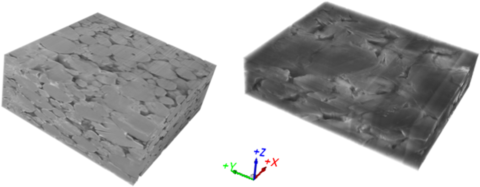
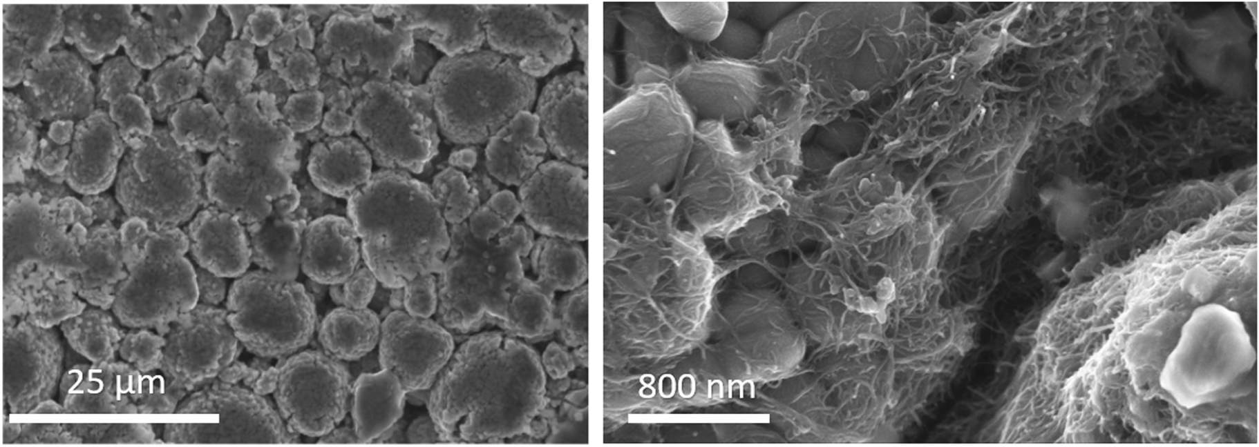
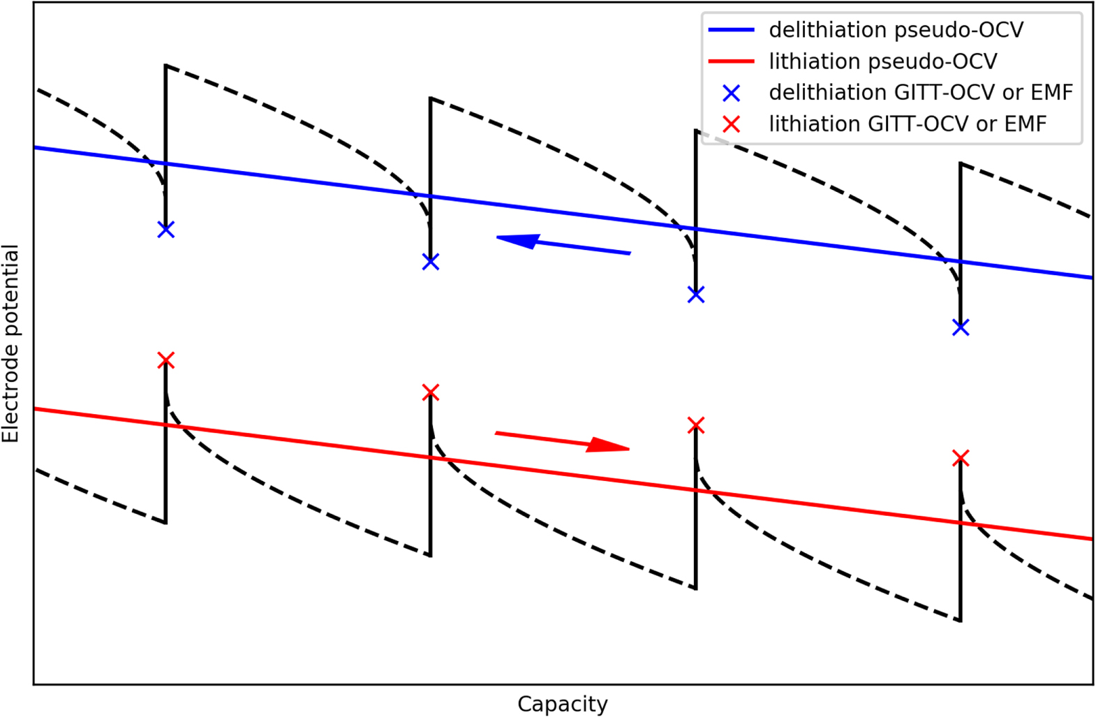
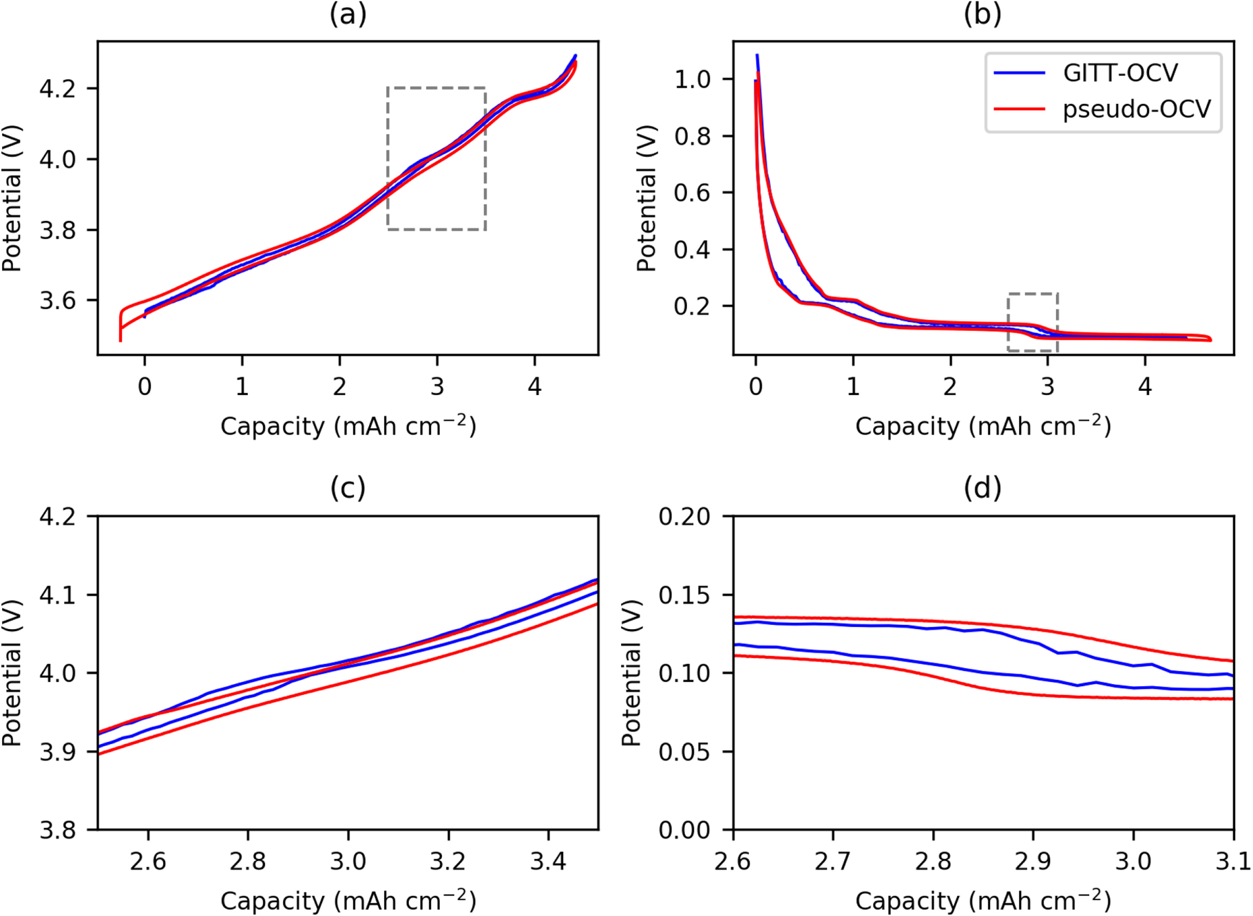
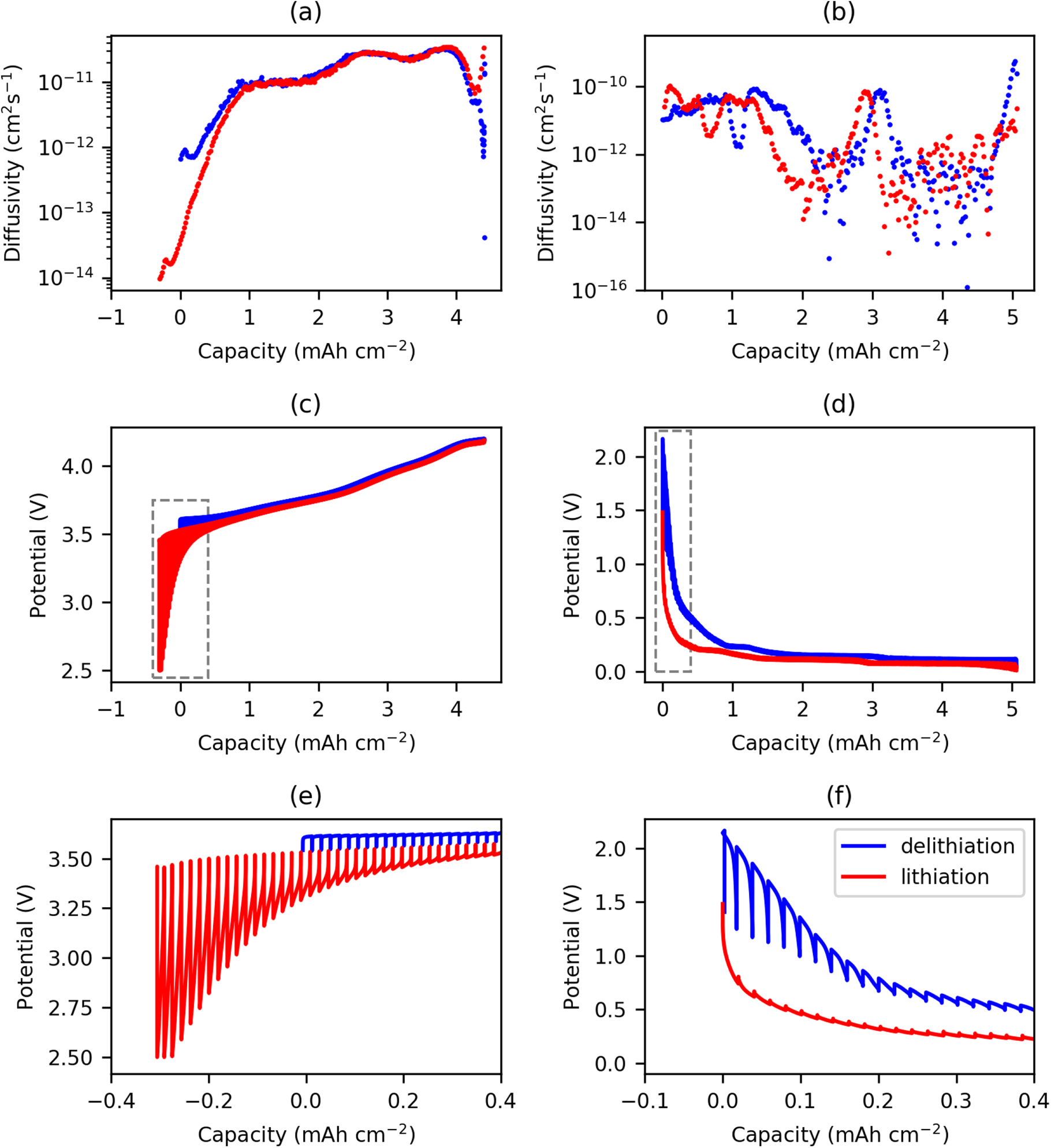
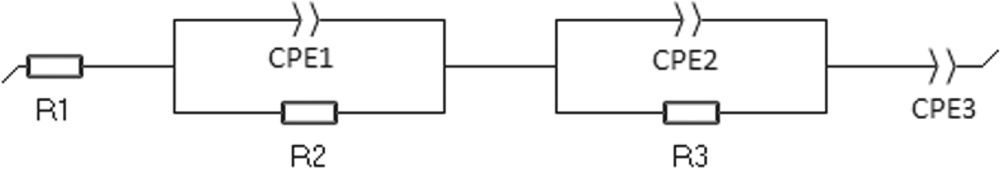
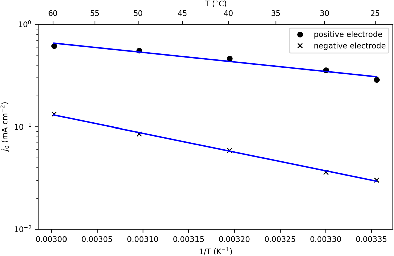
Figure 17. Comparison between the P2D simulations and the experimental data for C/2 (top), 1C (middle) and 1.5C (bottom). The plots on the left show the simulated and the measured output voltages, while the plots on the right show the voltage error as a function of time. The parameters are the same for the three C-rates, except for the diffusion coefficient in the negative electrode which is adjusted for each C-rate.
Download figure:
Standard image High-resolution image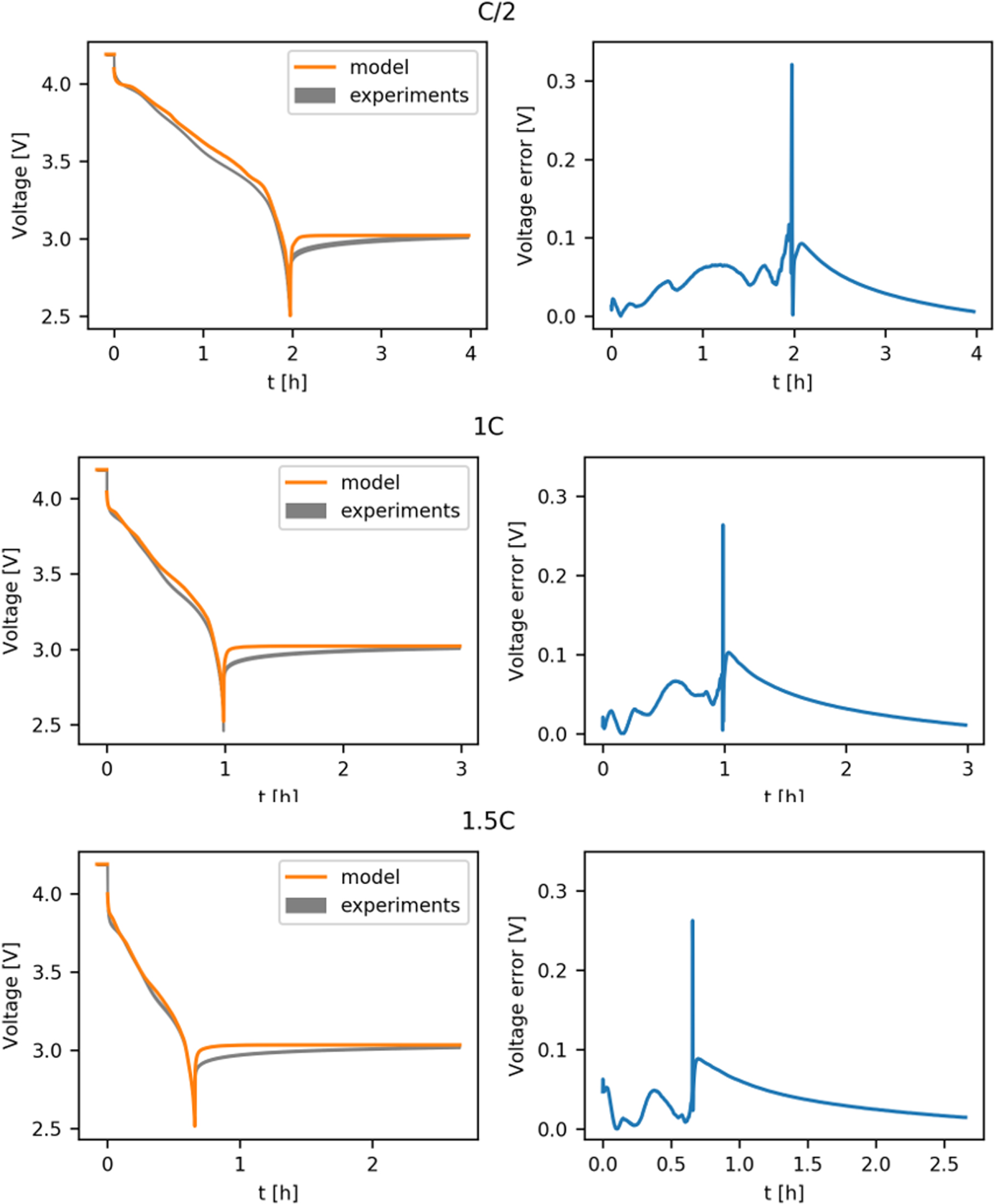
Good agreement between experiments and simulations is observed, especially considering that only eight of the more than 30 parameters in the model had to be adjusted, and three of them (Bruggeman coefficients in both electrodes and separator) were set to their theoretical value rather than tuned. The model captures well the discharge profile and the final voltage after the relaxation period. The transient at the beginning of the relaxation is not quite well captured, probably due to the assumption of linear diffusion in the model. Looking at the error plots we notice that the peak error is at the end of discharge, however, the main contributions to the RMSE are during relaxation. This links to a very important point in the parameter validation, as we found that varying the diffusion coefficients leads to minor variations in the error during discharge, but to a significant increase of the error during relaxation, which notably contributes to the RMSE. Therefore, we highlight the importance of including a relaxation period when comparing simulation results with experimental data.
Notice that all the parameters adjusted are related to the porous electrode. These results also suggest that in order to capture the electrode inhomogeneity, other parameters could be taken as effective parameters, for example the particle radius, instead of the diffusion coefficients. This is an area for further work.
Discussion upon testing methods
The teardown process may affect the integrity of the components of the cell. The cell has a unique eco-system which is sealed to the environment, and as soon as the cell is opened this is compromised. We have tested the validity of these tear down processes by comparing the observed voltage profiles in a LGM50 cell with those observed in a reassembled cell. The areal capacity we observe for the positive electrode in the LGM50 cell is 4.88 mAh cm−2 and in a small format assembled cell is 4.7 mAh cm−2. This gives a good reflection of the potential damage occurs by cutting our small electrodes from the larger. However the difference is minimal (3.6%) which gives us a good indication that we are not affecting the performance of the electrodes significantly after tear down. The SEI layer may also be compromised upon the removal of the electrode, and therefore reconditioning of the electrodes was performed through two low rate cycles before any subsequent testing. This reconditioning regime was chosen as standard, because no significant change in the capacity was observed after two cycles. We must also consider that in washing the electrode we are likely to remove some of the SEI layer, particularly on the negative electrode, and therefore a slight loss of lithium inventory may occur upon reformation of the SEI. This could be around 3%–5% depending upon the graphite. We show in a half cell that the graphite first cycle efficiency is typically 95%–98%, indicating some loss of lithium. In this work we have not included the carbon and binder additive in the calculations and have assumed a 100% active mass. The contribution of these additives will be small, typically between 2%–5%, but this will add in a small error to the concentration values. Porosity will change depending upon compression and state of charge: NMC has an anisotropic expansion, and contracts at the higher voltages. This change in volume is around 4%–6% depending upon the upper voltage limit and this change in porosity is not considered in the models. However, we have taken into consideration the increase in particle volume for lithiation of the negative electrode, and this has a significant impact upon the diffusion coefficients. It is difficult to measure the effective change in porosity in the electrode microstructure, which is also likely to occur during the lithiation process.
There is significant scope for further work in understanding how the change in porosity affects the diffusion of the electrodes upon cycling. In terms of the voltage curves the full cell curves from the cylindrical cell and the extracted electrodes in a three-electrode test show that at low rates these curves map onto each other very well, indicating that the thermodynamic (OCV) data reflects that in the cylindrical cell well. Two main differences between the assembled cells and the commercial cell are the electrolyte and the separator used. We chose a standard 1 mol dm−3 concentration electrolyte, whereas the concentration is likely to be slightly higher (up to 1.2 mol dm−3) and likely with different solvents or additives. The change in concentration will affect the open circuit potential of each electrode separately, however the full cell data should remain the same as the shift in voltage will be reflected on both the negative and positive electrodes. The separator utilised in the reference cell is significantly thicker than that in the commercial cell, in order to obtain a stable reference voltage. Therefore, higher rate testing does not reflect that observed in the commercial cell due to the increase in polarization and is therefore not reported here. The concentration of the electrolyte and the separator design will affect the diffusion of the lithium ions in the electrolyte, and change the observed cell resistance. For the diffusion coefficient data capture, low current pulses were utilised to minimise the polarisation from this increased resistance, and the end of the current pulse was utilised in the Sand equation, to minimise any effects of the electrolyte and separator. We assume here that only diffusion occurring in the active materials is observed, as this is the limiting diffusivity of the cell, not the electrolyte ionic conductivity in the separator. The interpretation of the tortuosities in terms of the Bruggeman exponent is required by PyBAMM as it uses the Bruggeman correlation in the program, despite the unreliable theory.81 Therefore, we have utilised an exponent of 1.5 rather than those which were calculated as this describes the spherical nature of the electrode particles. A second method for calculation of the tortuosity is from the EIS data,82 and the contribution to the resistivity from the electrolyte and the separator can be extracted. If the contribution of the internal resistances to the polarisation or over potentials is better understood, we can improve the ability to predict how a cell chemistry will operate in different form factors. This is the subject of further work. It should be highlighted all the validation voltage profiles are from the LGM50 cylindrical cell. Therefore some level of tuning is expected due to the differences between the commercial separator and electrolyte, and the test cells, especially at higher rates.
Conclusions
We present here an extensive 35 parameter set of a commercial cylindrical 21700 cell (LGM50) cell, for an electrochemical pseudo-two-dimensional (P2D) model. The chemical, physical and electrochemical properties are extracted and derived through careful tear down analysis of the cells components, with no prior knowledge of the cell make-up.
The composition of the positive and negative electrode components were aluminium doped NMC 811 with carbon fiber conductive additive on aluminium, and a bi-component negative electrode of 90% graphite −10% SiOx negative electrode on copper. Similar active material volumes are evaluated through FIB-SEM 3D reconstruction and physical measurements with assumed material densities. Porosities of 25% and 33.5% were elucidated for the negative and positive electrodes respectively. From the electrode composition analysis in conjunction with the thermodynamic data obtained from OCV measurements we are able to calculate the stoichiometry and lithium concentration in the electrodes at all states of charge. The data from the different cell set-ups was normalized for areal capacity for direct comparison. The three-electrode OCV represents the typical operating range of the full battery, while the half cell provides the points that we can map to a given stoichiometry. A comparison of the two methods showed that GITT-OCV exhibited less polarization especially at low state of charge compared to the pseudo-OCV. GITT-OCV also shows a hysteresis upon charge and discharge, particularly for the negative electrode indicating a difference between lithiation and delithiation species. The GITT-OCV provides accurate stoichiometry results of the working cell where both negative and positive electrode stoichiometries are fitted at the same time. The GITT-OCV was also subsequently utilized in the P2D model simulations.
The diffusion coefficients were calculated from the voltage transient during the current pulse in GITT. From a derivation of the Sand equation we were able to elucidate the change in diffusion coefficient with state of charge for both positive and negative electrodes. One major simplification is upon the averaging of the particle sizes in the electrodes, in particular for the negative electrode which contains two phases. Both phases have very different particle sizes, current exchange densities and diffusion coefficients. The particle sizes of the graphite (5.86 μm) and silicon (1.52 μm) were obtained in the discharge state, therefore the average volume expansion of the electrode particles during lithiation could be estimated from the known expansion of the graphite (10%) and SiOx (118%). Utilizing an average particle size at 0% and 100% SOC an expansion factor was estimated and applied to the diffusion coefficient over the different SOC in order to compensate for the change in effective surface area as the particle volume increases.
The validity of the obtained parameters has been investigated by comparing experimental constant current discharge validation constant current data sets performed at room temperature, with simulated discharge from a P2D model using PyBaMM. After some minor tuning, the experimentally determined parameters give a good approximation and the model captures all of the voltage profile. However, the relaxation to OCV at the end of discharge was not reflected, indicating that the lithium transfer and hence the thermodynamic properties at end of discharge were not captured so well. Therefore, the three Bruggeman constants for the separator and electrodes were kept at the theoretical value of 1.5, and tuning was performed on five parameters relating to the diffusion coefficients, maximum concentrations and 100% stoichiometry in the positive electrode. These are the most sensitive parameters and we show changes to the parameters to be relatively minor in most cases with the largest tuning required for the negative electrode diffusion coefficient. The model currently uses a linear diffusion model for with a single effective diffusion coefficient for ease of calculation. As expected, the simulations here show limitations in assuming effective particle sizes, constant electrode porosity, diffusion coefficients and current exchange densities. In particular, the two-phase negative electrode (graphite and SiOx) requires a different approach to accurately simulate (and calculate) the lithium transport properties. However, a good approximation is provided by this work. For future models, we recommend using the variable diffusion coefficients, particle size distributions and variable electrode volume to better represent the electrode properties in the models.
In summary, we provide a 35-parameter data set for a LG M50 21700 cylindrical cell, the chemical composition and the physical dimensions of the internal components. The porosity, lithium concentration and stoichiometry of the negative and positive electrodes is presented. In addition we have elucidated the current exchange density and diffusion coefficients over the complete state of charge of the battery for each electrode. In particular, we present a full set of diffusion coefficient data set relating to a bi-component negative electrode, which undergoes volume expansion upon cycling.
Acknowledgments
We acknowledge the funding support received from Faraday Institution (faraday.ac.uk; EP/S003053/1), grant number FIRG003. The authors acknowledge Dr. Mike Lain for data analysis and discussion and Dr. David Burnett for the help in ICP-OES setup. We also thank Dr. Ivan Korotkin for the useful discussions regarding the fitting of the OCV curves.
Data availability—The parameter set used in the simulations (including the measured open-circuit voltages as function of the stoichiometry) are available in the Python Battery Mathematical Modelling (PyBaMM) package as one of the default datasets. The package repository is https://github.com/pybamm-team/PyBaMM.