Theory of Multicomponent Phenomena in Cation-Exchange Membranes: Part II. Transport Model and Validation

Isothermal, isotropic, multicomponent mass transport is governed by the nonequilibrium thermodynamic driving force on species $i,$ ${{\boldsymbol{d}}}_{i},$ balancing against the drag forces between $i$ and all other species $j$ in the system. According to the Stefan-Maxwell-Onsager theory,^13,25,29

$$\begin{eqnarray}&&{{\boldsymbol{d}}}_{i},=\displaystyle \displaystyle \sum _{j\ne i}{K}_{ij}({{\boldsymbol{v}}}_{j}-{{\boldsymbol{v}}}_{i})\end{eqnarray} \tag{ 1 }$$

where ${K}_{ij}$ characterizes the friction between species $i$ and $j$ and ${{\boldsymbol{v}}}_{i}$ is the velocity of species $i.$ The driving force for transport is²⁹

$$\begin{eqnarray}&&{{\boldsymbol{d}}}_{i}={c}_{i}\left({\rm{\nabla }}{\mu }_{i}-\displaystyle \frac{{M}_{i}}{\rho }{\rm{\nabla }}p-{{\boldsymbol{X}}}_{i}+\displaystyle \frac{{M}_{i}}{\rho }\displaystyle \sum _{j}{{\boldsymbol{X}}}_{j}{c}_{j}\right)\end{eqnarray} \tag{ 2 }$$

where ${c}_{i},$ ${\mu }_{i},$ ${M}_{i},$ and ${{\boldsymbol{X}}}_{i}$ are, respectively, the concentration (defined later), electrochemical potential, molar mass, and external body force on species $i;$ $p$ is pressure, and $\rho$ is mass density. We account for electrostatic forces in the electrochemical potential ${\mu }_{i}$ rather than in a body force ${{\boldsymbol{X}}}_{i}.$ The membrane, species ${\rm{M}},$ is affixed to a support (e.g., a mesh or gasket) that imparts a pinning force ${{\boldsymbol{X}}}_{{\rm{M}}}.$ A force balance on the membrane dictates that this force is equal to the pressure in the membrane, ${\rm{\nabla }}p={c}_{{\rm{M}}}{{\boldsymbol{X}}}_{{\rm{M}}}.$^44–46 An explicit stress balance in the membrane specifies ${{\boldsymbol{X}}}_{{\rm{M}}}.$²⁰ Absent other external forces, substitution of Eq. 2 into Eq. 1 for each mobile species $i$ in the membrane relates the electrochemical potential gradients to species velocities^13,25,29

$$\begin{eqnarray}&&{c}_{i}{\rm{\nabla }}{\mu }_{i}={K}_{i{\rm{M}}}\left(-{{\boldsymbol{v}}}_{i}\right)+\displaystyle \sum _{j\ne i,{\rm{M}}}{K}_{ij}({{\boldsymbol{v}}}_{j}-{{\boldsymbol{v}}}_{i})\end{eqnarray} \tag{ 3 }$$

For $i={\rm{M}},$ isothermal Gibbs–Duhem demands that

$$\begin{eqnarray}&&{c}_{{\rm{M}}}{\rm{\nabla }}{\mu }_{{\rm{M}}}-{\rm{\nabla }}p=\displaystyle \sum _{i\ne {\rm{M}}}{K}_{i{\rm{M}}}{{\boldsymbol{v}}}_{i}\end{eqnarray} \tag{ 4 }$$

where ${{\boldsymbol{v}}}_{i}$ is a superficial velocity and ${K}_{ij}$ is the friction coefficient between species $i$ and $j.$ The electrochemical potential is a function of composition, pressure, temperature, $T,$ and electric state. The pressure gradient appears in Eq. 4 but not in Eq. 3 because of the pinning force on the membrane.^32,45,46 In Eqs. 3 and 4, the reference velocity is that of the membrane (i.e. ${{\boldsymbol{v}}}_{{\rm{M}}}=0$). Conservation of the membrane mass provides an additional constrain that relates ${{\boldsymbol{v}}}_{{\rm{M}}}$ to the laboratory frame of reference (i.e., to the support that affixes the membrane).⁴⁷ At steady state, the membrane is not actively swelling and the membrane velocity equals the velocity of the laboratory. We denote transport coefficients that depend on the frame-of-reference with a superscript of the reference species (i.e., ${\rm{M}}$). If the species are chemically independent (i.e., no reactions between them; the proceeding section lifts this restriction), then for $N$ species (including all species absorbed in the membrane and the membrane), there are $N-1$ independent equations of this form .²⁹ Eq. 3 in matrix form is¹³

$$\begin{eqnarray}&&{\boldsymbol{D}}={{\boldsymbol{M}}}^{{\rm{M}}}{\boldsymbol{V}}\end{eqnarray} \tag{ 5 }$$

where ${\boldsymbol{D}}$ and ${\boldsymbol{V}}$ are $N-1$ by 3 matrices in which the $i$th row contains, respectively, the components of the 3D vector of driving forces and velocities of species $i$ (i.e. ${D}_{i* }={c}_{i}{\rm{\nabla }}{\mu }_{i}$ and ${V}_{i* }={{\boldsymbol{v}}}_{{\boldsymbol{i}}},$ where the subscript $*$ denotes a row) excluding the row and column ${\rm{M}},$ due to linear dependence.⁴⁸ The transport coefficient matrix ${{\boldsymbol{M}}}^{{\rm{M}}}$ is $N-1$ by $N-1$ where ${M}_{ij}^{{\rm{M}}}={K}_{ij}$ for $i\ne j$ and ${M}_{ii}^{{\rm{M}}}=-\sum _{j\ne i}{K}_{ij}.$

Onsager reciprocal relations dictate that the friction coefficients are symmetric, ${K}_{ij}={K}_{ji}.$⁴⁸ Consequently, there are $N(N-1)/2$ friction coefficients. ${K}_{ij}$ coefficients are related to binary interspecies diffusion coefficients according to²⁵

$$\begin{eqnarray}&&{{\mathfrak{D}}}_{ij}=\displaystyle \frac{RT{c}_{i}{c}_{j}}{{K}_{ij}{c}_{{\rm{T}}}}\end{eqnarray} \tag{ 6 }$$

where ${c}_{{\rm{T}}}$ is the total molar concentration of the solution.

The molar concentration for a phase-separated membrane is defined either on a superficial basis (e.g., a homogenous phase) that includes the polymer volume (${c}_{i}^{{\prime} }={n}_{i}/\sum _{i}{n}_{i}{\bar{V}}_{i}\,$ where ${n}_{i}$ and ${\bar{V}}_{i}$ are the moles and partial molar volume of species $i$), or an interstitial basis (e.g., heterogeneous phases) that only includes the electrolyte solution in the membrane pores (${c}_{i}={n}_{i}/\sum _{i\ne {\rm{M}}}{n}_{i}{\bar{V}}_{i}$). We use the latter definition because it is more amenable to microscopic theories of ${{\mathfrak{D}}}_{ij}$ that are derived for bulk electrolyte solutions or porous media. We neglect changes to the total molar concentration ${c}_{{\rm{T}}}$ in the hydrophilic domains; the molar concentration of species $i$ is ${c}_{i}={c}_{{\rm{T}}}({n}_{i}/\sum _{j\ne {\rm{M}}}{n}_{j})$ where ${c}_{{\rm{T}}}$ is set to the molar concentration of salt-free water at 25 °C, (=55.2 mol dm⁻³). This assumption is rigorously valid for high water contents ($\lambda \gt 10$) or for membranes exchanged with cations that have molar volumes similar to water.

Many ionic species undergo ion-pair or acid-base equilibria that alter transport properties.⁴⁹ Transport measurements typically control amounts of neutral components added to the system and treat the $N$ constituent ionic species as fully dissociated in solution (we call this the "Experimental Construct" and denote quantities in the construct with superscript exp). For example, sulfuric acid is treated as protons and sulfate ions. The Experimental Construct provides independent driving forces and fluxes for species. However, because friction between species depends on size and charge, microscopic models consider ${N}^{{\rm{mol}}}$ species in their actual, associated states (we call this the "Molecular Construct" and denote quantities in this construct with superscript ${\rm{mol}}$). For example, sulfuric acid is treated as protons, bisulfate, and sulfate ions.⁴²

By accounting for how driving forces in the Molecular Construct are interdependent, Appendix A shows that the friction-coefficient matrix in the Molecular Construct, ${{\boldsymbol{M}}}^{{\rm{M}}{\rm{mol}}}$ (a ${N}^{{\rm{mol}}}-1$ by ${N}^{{\rm{mol}}}-1$ matrix), is related to friction coefficients in the Experimental Construct, ${{\boldsymbol{M}}}^{{\rm{M}}\exp }$ according to

$$\begin{eqnarray}&&{{\boldsymbol{M}}}^{{\rm{M}}\exp }={\left({\boldsymbol{F}}{\left[{{\boldsymbol{M}}}^{{\rm{M}}\mathrm{mol}}\right]}^{-1}{{\boldsymbol{F}}}^{T}\right)}^{-1}\end{eqnarray} \tag{ 7 }$$

where ${\boldsymbol{F}}$ is a $N-1$ by ${N}^{{\rm{mol}}}-1$ matrix with $i,$ $j$ entries ${f}_{i,j},$ and ${f}_{i,j}$ is the fraction of moles of species $i$ in the Experimental Construct, ${n}_{i}^{\exp },$ that partially associates into ${n}_{j}^{{\rm{mol}}}$ moles of species $j$ in the Molecular Construct

$$\begin{eqnarray}&&{f}_{i,j}=-\displaystyle \frac{{n}_{j}^{{\rm{mol}}}{s}_{i}}{{n}_{i}^{\exp }{s}_{j}}\end{eqnarray} \tag{ 8 }$$

Here, ${s}_{i}$ and ${s}_{j}$ are the stoichiometric coefficients of species $i$ and $j,$ respectively, in the reaction of $i$ associating with another species to form $j.$ For example, protons (species $i$) associating with sulfate ions to form bisulfate ions (species $j$). Note that ${\sum }_{j}{f}_{i,j}=1.$ Theory gives the Molecular Construct transport coefficients (e.g., ${{\boldsymbol{M}}}^{{\rm{M}}{\rm{mol}}}$) that we convert to the Experimental Construct transport coefficients (e.g., ${{\boldsymbol{M}}}^{{\rm{M}}\exp }$) to calculate measured transport properties. In Part III,⁵⁰ it is more convenient to make calculations using Eq. 3 in the Experimental Construct. In that case, ${{\boldsymbol{M}}}^{{\rm{M}}\exp }$ provides ${{\mathfrak{D}}}_{ij}^{\exp }$'s according to the definition of ${{\boldsymbol{M}}}^{{\rm{M}}}.$ For convenience, we drop the superscript $\exp$ outside this section for quantities in the experimental construct.

In a liquid solution consisting of solvent and ionic species in a membrane, there are six types of friction coefficients: ion/solvent, cation/anion, cation/cation, anion/anion, ion/membrane, and solvent/membrane.^13,42,51,52 All but the last two types are present in bulk electrolyte solutions.⁵¹ Accordingly, we use measurements of friction coefficients in bulk solution and apply common theories for their compositional dependence to calculate their value in the hydrophilic domains of the membrane. This approach requires that the distance over which these molecular interactions occur is smaller than the size of the hydrophilic domains; this assumption is justified for the highly concentrated solutions in the membrane that strongly screen hydrodynamic influences and electrostatic interactions. A hydrodynamic model of membrane pores gives ion/membrane and solvent/membrane friction coefficients. The transport coefficients are scaled by the tortuosity $\tau$ and volume fraction, $1-{\phi }_{{\rm{M}}},$ of the hydrophilic membrane domains to relate the transport coefficients of a single hydrophilic domain to effective, superficial membrane fluxes used in Eqs. 3 and 4.⁵³ Tortuosity scales according to Archie's law, $\tau ={\left(1-{\phi }_{{\rm{M}}}\right)}^{-\chi },$ where $\chi$ is the tortuosity scaling parameter.⁵⁴ ${\phi }_{{\rm{M}}}$ is the volume fraction of the polymer backbone ($={\bar{V}}_{{\rm{M}}}/({\bar{V}}_{{\rm{M}}}+{\bar{V}}_{0}{n}_{0}/{n}_{{\rm{M}}}\,)$ neglecting the volume of absorbed ions in the membrane), ${\bar{V}}_{{\rm{M}}}$ is the partial molar volume of polymer per charged group (=523.8 cm³/mole-SO₃⁻ for Nafion).² $\chi$ is independent of water content and electrolyte concentration in the membrane.

For ion/solvent friction coefficients, the Stokes-Einstein equation predicts the changes with solution viscosity of the binary diffusion coefficient as a result of the drag of an ion, idealized as a sphere, moving (or rotating) through a stagnant continuum solvent⁴²

$$\begin{eqnarray}&&{{\mathfrak{D}}}_{i0}^{{\rm{mol}}}=\left(\displaystyle \frac{1-{\phi }_{{\rm{M}}}}{\tau }\right)\displaystyle \frac{{\eta }^{\infty }}{\eta }{{\mathfrak{D}}}_{i0}^{\infty \,{\rm{mol}}}\end{eqnarray} \tag{ 9 }$$

where $\eta$ is the solution viscosity and the superscript $\infty$ denotes infinite dilution. The term in parenthesis on the right side corrects the interstitial diffusion coefficient for the tortuosity and volume fraction of hydrophilic channels. The viscosity ratio arise because the solution becomes more viscous at high ionic strengths due to increased steric interactions between ions in solution. Einstein's viscosity equation predicts how solution viscosity changes with concentration⁵⁵

$$\begin{eqnarray}&&\eta =\displaystyle \frac{{\eta }^{\infty }\left(1+{\sum }_{i\ne 0,{\rm{M}}}^{{N}^{{\rm{mol}}}}{c}_{i}^{{\rm{mol}}}{\tilde{V}}_{i}/2\right)}{{\left(1-{\sum }_{i\ne 0,{\rm{M}}}^{{N}^{{\rm{mol}}}}{c}_{i}^{{\rm{mol}}}{\tilde{V}}_{i}\right)}^{2}}\end{eqnarray} \tag{ 10 }$$

where ${\tilde{V}}_{i}$ is the effective molar viscous volume of species $i,$ that is fit to electrolyte-solution viscosity data. Stokes–Einstein theory (Eq. 9) is widely used and generally effective at predicting the concentration dependence of ion-solvent diffusion coefficients, although agreement with experiment is imperfect.^24,25,42 In particular, Stokes-Einstein theory is inaccurate for associating electrolytes,²⁵ corrections of which are accounted for by using the Molecular Construct .

Although local viscous interactions govern ion/solvent friction, long-range electrostatics dominate ion/ion interactions.⁵⁶ A "cloud" of mostly oppositely charged ions surrounds an ion in solution.⁵⁶ When an external field is applied, that cloud distorts and exerts a retarding force on the ion opposing the external field.⁵⁶ From this resistive force, Debye-Hückel-Onsager theory predicts that in binary electrolytes the diffusion coefficient for oppositely charged ions varies with the square-root of concentration.^25,42

$$\begin{eqnarray}&&{{\mathfrak{D}}}_{ij}^{{\rm{mol}}}\propto \left(\displaystyle \frac{1-{\phi }_{{\rm{M}}}}{\tau }\right)\sqrt{{I}^{{\rm{mol}}}}\,\,\,\,\mathrm{for}\,\,\,{z}_{i\ne {\rm{M}},0}{z}_{j\ne {\rm{M}},0}\lt 0\end{eqnarray} \tag{ 11 }$$

where ${I}^{{\rm{mol}}}$ is the Molecular Construct ionic strength ($=\tfrac{1}{2}\displaystyle {\sum }_{i\ne 0,{\rm{M}}}^{{N}^{{\rm{mol}}}}{c}_{i}^{{\rm{mol}}}{z}_{i}^{2}$). Eq. 11 relates diffusion coefficients measured in bulk solution at a given ionic strength to those at other concentrations. Chapman⁴² and Wesselingh et al.⁵¹ suggested that, since the Debye-Hückel ion cloud is governed by the ionic strength in multicomponent electrolytes; Eq. 11 also applies to mixtures. Experiments agree with the Debye-Hückel-Onsager description that friction between similarly charged ions is negligible as they scarcely interact, or^13,51

$$\begin{eqnarray}&&{{\mathfrak{D}}}_{ij}^{{\rm{mol}}}\to \infty \,{\rm{for}}\,{z}_{i\ne {\rm{M}}}{z}_{j\ne {\rm{M}}}\gt 0.\end{eqnarray} \tag{ 12 }$$

Debye–Hückel–Onsager theory does not apply to ionic groups attached to the polymer membrane, since they are fixed and unable to form an ionic cloud around mobile ions.⁵¹ Still, the membrane exerts a frictional force on aqueous ions and solvent from microscale-viscous interactions with the membrane walls.⁵⁷ Microscale hydrodynamics predicts viscous interactions between a fluid and a solid wall.⁵⁸ Species velocities and concentrations discussed up to this point are macroscopic averages and correspond to experimentally measurable quantities. In developing a microscale hydrodynamic model, we invoke microscopic, local quantities that are not experimentally accessible and are denoted with a superscript ${\rm{loc}}.$

Appendix B shows that the area-averaged, superficial velocity ${v}_{z}$ through the membrane (through-direction denoted as the $z$-coordinate) where each mobile species is under an electrochemical potential gradient $\partial {\mu }_{i}/\partial z$ is

$$\begin{eqnarray}&&{v}_{z}=-\displaystyle \sum _{i\ne {\rm{M}}}^{{N}^{{\rm{mol}}}}\displaystyle \frac{{c}_{i}^{{\rm{mol}}}}{{{\mathscr{K}}}_{i}^{{\rm{mol}}}}\displaystyle \frac{\partial {\mu }_{i}}{\partial z}\end{eqnarray} \tag{ 13 }$$

where ${{\mathscr{K}}}_{i}^{{\rm{mol}}}$ is a hydrodynamic friction coefficient that satisfies the creeping-flow momentum balance in a pore with appropriate boundary conditions. By definition, ${v}_{z}$ is the sum of species velocities in the Molecular Construct ${v}_{i,z}^{{\rm{mol}}}$ weighted by their mass fractions ${w}_{i}^{{\rm{mol}}}$ (i.e., mass-averaged velocity, ${v}_{z}=\sum _{{N}^{{\rm{mol}}}}^{i\ne {\rm{M}}}{w}_{i}^{{\rm{mol}}}{v}_{i,z}^{{\rm{mol}}}$ where ${w}_{i}^{{\rm{mol}}}={n}_{i}^{{\rm{mol}}}{M}_{i}/\sum _{{N}^{{\rm{mol}}}}^{i\ne {\rm{M}}}{n}_{i}^{{\rm{mol}}}{M}_{i}$). In Appendix C, we demonstrate that the expression for ${K}_{i{\rm{M}}}^{{\rm{mol}}}$ that satisfies both the hydrodynamic prediction of Eq. 13 and frictional interactions in Eq. 3 is

$$\begin{eqnarray}&&{K}_{i{\rm{M}}}^{{\rm{mol}}}={w}_{i}^{{\rm{mol}}}{{\mathscr{K}}}_{i}^{{\rm{mol}}}+\sum _{j\ne {\rm{M}}}^{{N}^{{\rm{mol}}}}{K}_{ij}^{{\rm{mol}}}\left(\displaystyle \frac{{{\mathscr{K}}}_{i}^{{\rm{mol}}}}{{{\mathscr{K}}}_{j}^{{\rm{mol}}}}-1\right)\end{eqnarray} \tag{ 14 }$$

where the first term on the right is due to hydrodynamic interactions directly causing friction on species $i$ and the second term is due to hydrodynamic friction on species $j$ that, in turn, exerts friction ${K}_{ij}^{{\rm{mol}}}$ on $i.$

Following classic treatments of electrokinetics in microchannels,²⁵ Appendix B shows that for a translationally invariant pore forming a channel with tortuosity $\tau ,$ ${{\mathscr{K}}}_{i}^{{\rm{mol}}}$ is

$$\begin{eqnarray}&&{{\mathscr{K}}}_{i}^{{\rm{mol}}}=\displaystyle \frac{4G\eta }{{R}_{{\rm{pore}}}^{2}{\theta }_{i}}\left(\displaystyle \frac{\tau }{1-{\phi }_{{\rm{M}}}}\right)\end{eqnarray} \tag{ 15 }$$

where ${R}_{{\rm{pore}}}$ is the radius of the pore and is a function of the membrane polymer volume fraction, ${R}_{{\rm{pore}}}={d}_{0}{{\phi }}_{{\rm{M}}}^{-m}{\left(1-{{\phi }}_{{\rm{M}}}\right)}^{1/2}/2$,⁵⁹ ${d}_{0}$ is dry-membrane domain spacing (2.7 nm for Nafion) and $m$ is a swelling parameter determined from microstructural characterization (1.33 for Nafion).² $G$ is the semi-empirical geometric factor that accounts for pore shape and distribution of sizes of the hydrophilic channels, and is independent of membrane water content and ion concentration.⁵³ Just as in Eqs. 9 and 11, the term in parenthesis on the right side corrects the interstitial hydrodynamic coefficient for the tortuosity and volume fraction of hydrophilic channels. ${\theta }_{i}$ accounts for how species $i$ distributes across the channel and equals unity when $i$ is uniformly distributed.

To establish ${\theta }_{i},$ we treat the negatively charged polymer sulfonate groups as uniformly distributed along the channel walls. Because cations are solvated, they cannot approach the walls closer than their solvated radius (i.e., the outer Helmholtz plane),⁶⁰ which we set to the diameter of a water molecule $2{R}_{0}=0.275$ nm;⁶¹ Because this study deals with high membrane hydration levels where cations are fully solvated, we do not consider cation-membrane ion-pair formation (i.e., ions complexed with the surface by dehydrating and moving to the inner Helmholtz plane).⁶⁰ Consequently, ionic species are distributed across a pore of effective radius ${R}_{{\rm{pore}}}-2{R}_{0}$ according to the linearized Poisson-Boltzmann equation.⁶⁰ For this system, Appendix B shows that ${\theta }_{i}$ is given by

$$\begin{eqnarray}&&{{\theta }}_{i\ne 0}={{\beta }}^{2}\left(2-{{\beta }}^{2}-{z}_{i}{\varrho }\left({{\beta }}^{2}+\displaystyle \frac{8}{{\left({R}_{{\rm{pore}}}k\right)}^{2}}-\displaystyle \frac{4{\beta }{I}_{0}\left({R}_{{\rm{pore}}}k\right)}{{R}_{{\rm{pore}}}k{I}_{1}\left({R}_{{\rm{pore}}}k\right)}\right)\right)\end{eqnarray} \tag{ 16 }$$

where $\beta$ is the ratio of the effective pore radius traversed by ions after accounting for solvation and the true radius $\left({R}_{{\rm{pore}}}-2{R}_{0}\right)/{R}_{{\rm{pore}}},$ ${\varrho }$ is $\sum _{{N}^{{\rm{mol}}}}^{i\ne {\rm{M}}}{n}_{i}^{{\rm{mol}}}{z}_{i}/\,\sum _{{N}^{{\rm{mol}}}}^{i\ne {\rm{M}}}{n}_{i}^{{\rm{mol}}}{z}_{i}^{2},$ $k$ is inverse Debye length ($={\left(\sum _{{N}^{{\rm{mol}}}}^{i\ne {\rm{M}}}{c}_{i}^{{\rm{mol}}}{z}_{i}^{2}{F}^{2}/{\varepsilon }_{r}{\varepsilon }_{0}RT\right)}^{1/2}$), ${\varepsilon }_{r}$ is bulk solvent dielectric constant (= 78.3), ${\varepsilon }_{0}$ is vacuum permittivity, and ${I}_{0}$ and ${I}_{1}$ are modified Bessel functions of the first kind with order 0 and 1, respectively. We neglect changes in solvent concentration across the pore so that ${\theta }_{0}=1.$

Equations 3 and 4 provide a microscopic description of multi-ion transport in membranes that relate species fluxes to driving forces, whereas experiments obey a macroscopic description in which experimentally controlled driving forces cause species fluxes. Fuller showed that Eq. 5 inverts to a macroscopic form³²

$$\begin{eqnarray}&&{{\boldsymbol{N}}}_{i}=-\displaystyle \sum _{j\ne {\rm{M}}}{L}_{ij}^{{\rm{M}}}{c}_{i}{c}_{j}{\rm{\nabla }}{\mu }_{j}\end{eqnarray} \tag{ 17 }$$

where ${{\boldsymbol{N}}}_{i}$ is the molar flux vector of species $i\ne {\rm{M}}$ and ${L}_{ij}^{{\rm{M}}}$ is a component of the $N-1$ by $N-1$ symmetric matrix ${{\boldsymbol{L}}}^{{\rm{M}}}$ defined as^32,53

$$\begin{eqnarray}&&{{\boldsymbol{L}}}^{{\rm{M}}}=-{\left({{\boldsymbol{M}}}^{{\rm{M}}}\right)}^{-1}\end{eqnarray} \tag{ 18 }$$

where the membrane, species ${\rm{M}},$ is used as a reference.

Because experimental measurements rarely ascertain the ${L}_{ij}^{{\rm{M}}}$ transport coefficients directly, we rewrite Eq. 17 in terms of transport coefficients that are measureable under well-defined experimental conditions, such that in terms of a controlled gradient of electrochemical potential ${\mu }_{n}$^13,25

$$\begin{eqnarray}&&{{\boldsymbol{N}}}_{i}=-\displaystyle \frac{{t}_{i}^{{\rm{M}}}\kappa }{{z}_{i}{F}^{2}}\displaystyle \frac{{\rm{\nabla }}{\mu }_{n}}{{z}_{n}}-\displaystyle \sum _{j\ne {\rm{M}}}\left({\alpha }_{ij}^{{\rm{M}}}+\displaystyle \frac{{t}_{i}^{{\rm{M}}}{t}_{j}^{{\rm{M}}}\kappa }{{z}_{i}{z}_{j}{F}^{2}}\right){\rm{\nabla }}{\mu }_{j,n}\end{eqnarray} \tag{ 19 }$$

or, equivalently, in terms of a controlled current density

$$\begin{eqnarray}&&{{\boldsymbol{N}}}_{i}=\displaystyle \frac{{t}_{i}^{{\rm{M}}}{\bf{i}}}{{z}_{i}F}-\displaystyle \sum _{j\ne {\rm{M}}}{\alpha }_{ij}^{{\rm{M}}}{\rm{\nabla }}{\mu }_{j,n}\end{eqnarray} \tag{ 20 }$$

where $F$ is Faraday's constant, ${z}_{i}$ is the charge number of species $i,$ ${t}_{i}^{{\rm{M}}}$ is the transference number of species $i,$ $\kappa$ is conductivity, and ${\alpha }_{ij}^{{\rm{M}}}$ is the transport coefficient between species $i$ and $j.$ In the absence of concentration, pressure, or temperature gradients, for a charged species $i,$ ${\rm{\nabla }}{\mu }_{i}={z}_{i}F{\rm{\nabla }}{\rm{\Phi }},$ where ${\rm{\Phi }}$ is the electric potential. To avoid invoking an arbitrary definition of ${\rm{\nabla }}{\rm{\Phi }}$ when there are concentration gradients, Eqs. 19 and 20 use ${\mu }_{i,n},$ the chemical potential of species $i$ relative to that of species $n,$ ${\mu }_{i,n}={\mu }_{i}-\tfrac{{z}_{i}}{{z}_{n}}{\mu }_{n}.$ ${\mu }_{i,n}$ is independent of ${\rm{\Phi }},$ depending only on the thermodynamic variables pressure, concentration, and temperature.²⁵ The first terms on the right sides of Eqs. 19 and 20 specify flux due to concentration and pressure gradients and the second terms specifies transport due to migration. Because protons are present in numerous applications of cation-exchange, a convenient choice for $n$ is ${{\rm{H}}}^{+}.$¹³

Equations 19 and 20 are general for isothermal transport. The transport coefficients appearing in these equations are related to the ${L}_{ij}^{{\rm{M}}}$'s and are material properties of the polymer membrane that for a set composition and temperature are independent of the applied driving forces. Under certain common experimental conditions, these properties have a clear physical interpretation. Specifically, ionic conductivity, $\kappa ,$ and $N-2$ transference numbers, ${t}_{i}^{{\rm{M}}},$ relate the fluxes and current to the applied electric potential in the absence of concentration, temperature and pressure gradients

$$\begin{eqnarray}&&\begin{array}{l}{\bf{i}}=-\left(\kappa \right){\rm{\nabla }}{\rm{\Phi }}=-\left({F}^{2}\displaystyle \sum _{i\ne {\rm{M}}}\sum _{j\ne {\rm{M}}}{L}_{ij}^{{\rm{M}}}{z}_{i}{c}_{i}{z}_{j}{c}_{j}\,\right){\rm{\nabla }}{\rm{\Phi }},\\ \,{\rm{for}}\,{\rm{\nabla }}{c}_{i}={\rm{\nabla }}T={\rm{\nabla }}p=0\end{array}\end{eqnarray} \tag{ 21 }$$

and

$$\begin{eqnarray}&&\begin{array}{l}{{\boldsymbol{N}}}_{i}=\left(\frac{{t}_{i}^{{\rm{M}}}}{{z}_{i}}\right)\frac{{\bf{i}}}{F}=\left(\frac{{c}_{i}{F}^{2}}{\kappa }\displaystyle \sum _{j\ne {\rm{M}}}{L}_{ij}^{{\rm{M}}}{z}_{j}{c}_{j}\right)\frac{{\bf{i}}}{F},\\ \,\,\mathrm{for}\,{\rm{\nabla }}{c}_{i}={\rm{\nabla }}T={\rm{\nabla }}p=0\end{array}\end{eqnarray} \tag{ 22 }$$

where the second equality provides $\kappa$ and ${t}_{i}^{{\rm{M}}}$ in terms of the ${L}_{ij}^{{\rm{M}}}$'s. The electroosmotic coefficient is related to the transference number of water by the ratio ${t}_{0}^{{\rm{M}}}/{z}_{0}=\xi ,$ which is finite even though ${z}_{0}=0.$¹³ Similarly, ${\alpha }_{ij}^{{\rm{M}}}$ has a straightforward physical interpretation for experiments in the absence of current; ${\alpha }_{ij}^{{\rm{M}}}$ is the proportionality constant relating species fluxes under chemical potential gradients absent net ionic current (${\bf{i}}=0$) and relate to ${L}_{ij}^{{\rm{M}}}$ according to¹³

$$\begin{eqnarray}&&\begin{array}{l}{{\boldsymbol{N}}}_{i}=-{\alpha }_{ij}^{{\rm{M}}}{\rm{\nabla }}{\mu }_{j,n}=-\left({L}_{ij}^{{\rm{M}}}{c}_{i}{c}_{j}-\displaystyle \frac{{t}_{i}^{{\rm{M}}}{t}_{j}^{{\rm{M}}}\kappa }{{z}_{i}{z}_{j}{F}^{2}}\right){\rm{\nabla }}{\mu }_{j,n}\\ \,{\rm{for}}\,{\bf{i}}=0\end{array}\end{eqnarray} \tag{ 23 }$$

where ${\alpha }_{ij}^{{\rm{M}}}$ is symmetric, which gives $(N-1)N/2\,$ ${\alpha }_{ij}^{{\rm{M}}}$'s of which $(N-2)(N-1)/2$ are independent.

The transmissibility of the membrane to water, ${L}_{{\rm{trans}},0},$ dictates the superficial velocity of water through the membrane under an applied pressure gradient. The solvent/solvent transport coefficient, ${\alpha }_{00}^{{\rm{M}}},$ relates to measured ${L}_{{\rm{trans}},0},$ as.¹³

$$\begin{eqnarray}&&{L}_{{\rm{trans}},0}\approx {\alpha }_{00}^{{\rm{M}}}\displaystyle \frac{{\bar{V}}_{0}^{2}}{l}\end{eqnarray} \tag{ 24 }$$

where the membrane thickness, $l,$ increases with water content from the dry thickness, ${l}^{0};$ for isotropic swelling $l={l}^{0}{\left(1+\tfrac{{n}_{0}{\bar{V}}_{0}}{{n}_{{\rm{M}}}{\bar{V}}_{{\rm{M}}}}\right)}^{\displaystyle \frac{1}{3}}.$² Equation 24 is approximate because neglects volume change on mixing of the water and membrane and neglects ionic contributions to the volume of the solution.

Literature reports values of $\kappa$ and, less frequently, $\xi ,$ ${t}_{{{\rm{H}}}^{+}}^{{\rm{M}}},$ and ${L}_{{\rm{trans}},0}$ for PFSA membranes. Here, we consider properties of membranes that are immersed in aqueous electrolyte solutions where membrane water content is relatively high. To calculate measured properties with the proposed model for a membrane in bulk solution at a given composition, we first calculate the water volume fraction ${\phi }_{0}$ (neglecting the volume of ions, ${\phi }_{0}=1-{\phi }_{{\rm{M}}}$) and molality of ions in the membrane ${m}_{i}$ and the speciation of associating ions ${f}_{i,j}$ from chemical-equilibrium relations outlined in Part I.⁴³ Although this calculation is self-consistent, model and experimental errors in electrolyte partitioning propagate to measurements and predictions of the transport properties. We relate the membrane composition to the chemical potentials of the external environment using an equilibrium model. In the steady state, we need not include a viscoelastic response of the polymer, which may be required in a transient simulation.²

Equations 6, 9, 11, and 12 give ${K}_{ij}^{{\rm{mol}}}$ for species $i$ and $j$ excluding the membrane ${\rm{M}}$ while Eq. 14 gives ${K}_{i{\rm{M}}}^{{\rm{mol}}}.$ The ${K}_{ij}^{{\rm{mol}}}$'s specify ${{\boldsymbol{M}}}^{{\rm{M}}{\rm{mol}}}$ and Eq. 7 gives ${{\boldsymbol{M}}}^{{\rm{M}}}.$ Inversion of ${{\boldsymbol{M}}}^{{\rm{M}}}$ following Eq. 18 provides ${{\boldsymbol{L}}}^{{\rm{M}}}.$ The components of ${{\boldsymbol{L}}}^{{\rm{M}}}$ give measured transport properties outlined in Eqs. 21–23. Matrix inversions are performed using the Python package NumPy version 1.16.

Because of the wide availability of data, we restrict our investigation to the Nafion PFSA chemistry.^2,62–67 Specifically, we use data for Nafion versions N117, N115, N212, and N211. The different numbered membranes have the same molecular formulae but the N11x sequence is extruded, whereas the series N21x is cast from solution; x denotes thickness in units of mils.² For operating parameters, we use ambient temperature (298 K) and pressure (101.3 kPa). As discussed in Supplemental Material, measurements of bulk-solution transport provide most properties at these conditions (specifically, ${\tilde{V}}_{i},$ ${{\mathfrak{D}}}_{0i\ne {\rm{M}}}^{\infty {\rm{mol}}},$ and ${{\mathfrak{D}}}_{i\ne 0,{\rm{M}}j\ne 0,{\rm{M}}}^{{\rm{mol}}}$ at a reference concentration). Parameters of ions unavailable in the literature are set to those ions of similar charge number that are available (see SM).

Table I provides the two adjusted values for the parameters of Nafion membranes. These are Archie's tortuosity scaling parameter, $\chi ,$ and the geometric transport factor, $G.$ Results and Discussion show that the parameter values are the best eye-fit of calculated and measured membrane conductivity proton transference number, electroosmotic coefficient, and water-water transport coefficient. $G$ and $\chi$ are independent of membrane water and ion content, Results and Discussion compares model predictions with experiments.

Table I.  Nafion membrane specific fitting parameters in the model.

Parameters	Value [−]
$\chi$	0.3 for data from62–64,68
	1.2 otherwise
$G$	4

Since membrane pretreatment and processing impact network tortuosity,² we use two values of Archie's parameter: $\chi =0.3$ for the highly pretreated and conductive N117 and N115 membranes measured by Okada and co-workers reported to have a proton-form conductivity of ∼0.2 S cm⁻¹ in liquid water ^62–64,68, and $\chi =1.2$ for all other datasets that consistently report $\kappa$ < 0.1 S cm⁻¹ for proton-form membranes in liquid water at room temperature.^65,69,70 Both of these values fall within the range of $\chi$ for a range of different types of porous media (0.3–3.4)⁷¹. $G$ for different pore shapes falls between 2 and 3, which correspond to circular- and slit-pore shape cross sections, respectively.⁵³ This range of $G$ is lower than the value fit here. The discrepancy is likely due an extremely heterogeneous distribution of hydrophilic domain sizes that leads to a large effective $G.$⁵³ Porous media with parallel-type pore nonuniformities in which species transport through pores that are larger than average lead to $G$'s that are greater than those predicted by pore shape alone.⁵³

Okada et al.^62–64,68 extensively characterized transport properties of N115 and N117 by measuring conductivity $\kappa ,$ proton and lithium transference numbers ${t}_{i}^{{\rm{M}}},$ electroosmotic coefficient $\xi ,$ and water transport coefficient ${\alpha }_{00}^{{\rm{M}}}$ of membranes that are partially exchanged with different cations in liquid aqueous electrolytes.

The mathematical model outlined in Part I⁴³ calculates the water volume fraction ${\phi }_{0}$ and molality of species in the membrane ${m}_{i}$ (given in Figs. 4, 5 and S1 in Part I). Given these values, we calculate the transport properties of mixed-exchanged proton-alkali Nafion membranes in liquid water. Figure 1 shows measured^63,73 (symbols) and calculated (lines) (a) membrane conductivity $\kappa ,$ (b) proton transference number ${t}_{{{\rm{H}}}^{+}}^{{\rm{M}}},$ (c) electroosmotic coefficient $\xi ,$ (d) and water transport coefficient ${\alpha }_{00},$ (e) ion-water transport coefficient ${\alpha }_{i0}^{{\rm{M}}}$ (not measured, only calculated), and (f) ion-ion transport coefficient ${\alpha }_{ij}^{{\rm{M}}}$ (not measured, only calculated) as function of the fractional proton exchange ${n}_{{{\rm{H}}}^{+}}/{n}_{{{\rm{SO}}}_{3}^{-}}$ (i.e. the fraction of negatively charged polymer sulfonate group charge-balanced by protons) with various alkali metal cations. For membranes partially exchanged with alkali cations and protons, the transport coefficients are related according to ${\alpha }_{0{{\rm{A}}}^{+}}^{{\rm{M}}}=-{\alpha }_{0{{\rm{H}}}^{+}}^{{\rm{M}}}$ and ${\alpha }_{{H}^{+}{H}^{+}}^{{\rm{M}}}=-{\alpha }_{{A}^{+}{H}^{+}}^{{\rm{M}}}={\alpha }_{{A}^{+}{A}^{+}}^{{\rm{M}}}.$¹³ Best-eye fitting of the data in Fig. 1 specifies $\chi$ and $G.$ Figure S1 shows the same calculated transport properties as Fig. 1 for lithium-form membrane exchanged with other alkali cations (${\alpha }_{00}$ not measured).⁶² The fitted $\chi$ and $G$ in Table I calculate transport properties for mixed lithium-alkali form membranes without adjustment.

Zoom In Zoom Out Reset image size

Agreement in Fig. 1 between theory and experiment is sufficient for differing membrane proton fractions and ion types. There are three cases that the model differs from experiment. The model calculates a higher sodium-exchanged membrane conductivity than does the measurement. We attribute this difference to varying experimental conditions because the measured sodium-exchanged samples have lower conductivity than the other cation-exchanged samples even when the membranes are fully in proton form (i.e. they should have identical composition), as Fig. 1a shows.^63,73 The model significantly over-predicts ${\alpha }_{00}^{{\rm{M}}}$ for the lithium-exchanged membranes, as Fig. 1d shows, and $\xi$ for partial cesium-exchanged membranes as Fig. 1c shows. These discrepancies may be partially attributed to the high experimental uncertainty for ${\alpha }_{00}^{{\rm{M}}}$ (calculated to be ∼40% for proton-form membranes in Fig. 1d) and to lack of experimental data. Further, we assume $G$ and $\chi$ are independent of cation type, but cation-sulfonate interactions can alter the membrane microstructure causing disagreement between calculated and measured transport properties.^74–76

As the membrane exchanges from alkali cation form to proton form, conductivity increases, plotted in Fig. 1a, because protons are much more mobile than alkali cations. Figure 1b shows that the high mobility of protons causes high ${t}_{{{\rm{H}}}^{+}}^{{\rm{M}}}$ except in membranes that are mostly exchanged with alkali cations (>50% exchanged). Equations 21 and 22 show that conductivity increases as Nafion exchanges from alkali ions to protons and $\xi$ decreases, consistent with Fig. 1c.

The high mobility of protons generates less friction for water transport through the membrane (see Eq. 6). A rising ${n}_{{{\rm{H}}}^{+}}/{n}_{{{\rm{SO}}}_{3}^{-}}$ ratio thus increases ${\alpha }_{00}^{{\rm{M}}},$ as Fig. 1d confirms. In the absence of current, low-mobility alkali cations move down a gradient chemical potential of water as they are dragged by water, but a streaming potential develops to ensure electroneutrality and causes highly mobile protons to move up a water chemical potential gradient (i.e., ${\alpha }_{0{{\rm{A}}}^{+}}^{{\rm{M}}}\gt 0$ and ${\alpha }_{0{{\rm{H}}}^{+}}^{{\rm{M}}}\lt 0$).

Figure 1e shows that in fully alkali ion-exchanged membranes, protons are not available to move in the opposite direction as alkali-cations and ${\alpha }_{0{{\rm{A}}}^{+}}^{{\rm{M}}}={\alpha }_{0{{\rm{H}}}^{+}}^{{\rm{M}}}=0.$ Similarly, ${\alpha }_{0{{\rm{A}}}^{+}}^{{\rm{M}}}={\alpha }_{0{{\rm{H}}}^{+}}^{{\rm{M}}}=0$ for fully proton-exchanged membranes. Figure 1f illustrates that ${\alpha }_{{{\rm{H}}}^{+}{{\rm{A}}}^{+}}^{{\rm{M}}}$ similarly reaches a maximum for partially exchanged membranes and is zero for fully exchanged membranes. The values of ${\alpha }_{00}^{{\rm{M}}}$ are more than an order of magnitude greater than $| {\alpha }_{i0}^{{\rm{M}}}|$ and $| {\alpha }_{ij}^{{\rm{M}}}| ,$ which demonstrate that fluxes induced by chemical-potential gradients of ions are secondary to those induced by an equal magnitude water chemical potential gradient.

The general trends described in the preceding two paragraphs hold for all membranes exchanged with each of the alkali cations. Variations in transport properties between the different alkali ions ${{\rm{A}}}^{+}$ are due to different ion-water binary diffusion coefficient at infinite dilution ${{\mathscr{D}}}_{0{{\rm{A}}}^{+}}^{\infty }$ (given in SM), to the water volume fraction of the exchanged membrane ${\phi }_{0}$ (given in Part I⁴³), and to the molar viscous volume of the cation-exchanged sample ${\tilde{V}}_{{{\rm{A}}}^{+}}$ (given in SM). ${\phi }_{0}$ decreases with increasing alkali cation crystallographic size (i.e. Li⁺ > Na⁺ > K⁺ > Cs⁺) and ${{\mathscr{D}}}_{0{{\rm{A}}}^{+}}^{\infty }$ has the opposite trend (i.e. Li⁺ < Na⁺ < K⁺ < Cs⁺). These different physical parameters explain the variations of transport properties in Fig. 1 for the different cation-exchanged membranes.

To explore these differences, Fig. 2 plots calculated transport properties for a 50% alkali ion-exchanged Nafion membrane (i.e. ${n}_{{{\rm{H}}}^{+}}/{n}_{{{\rm{SO}}}_{3}^{-}}$ = 0.5) on contour plots for (a) conductivity, (b) proton transference number, (c) electroosmotic coefficient, and (d) water, (e) ion-water, and (f) ion-ion transport coefficients as a function of ${\phi }_{0}$ on the y-axis and ${{\mathfrak{D}}}_{0{{\rm{A}}}^{+}}^{\infty }$ on the x-axis. Each x-y point in Fig. 2 are the transport properties of Nafion partially exchanged with a hypothetical alkali ion that has a diffusion coefficient ${{\mathfrak{D}}}_{0{{\rm{A}}}^{+}}^{\infty }$ and where the membrane water volume fraction is ${\phi }_{0}.$ For these calculations, we set all other properties of A⁺ (e.g., molar viscous volume and molar mass) to those of sodium because it is in the middle of the alkali series. To provide a reference, symbols in Fig. 2 are the ${{\mathfrak{D}}}_{0i}^{\infty }$ and ${\phi }_{0}$ for a 50% cation-exchanged Nafion membranes in liquid water for the different alkali cations.

Zoom In Zoom Out Reset image size

Figure 2a and 2f show that $\kappa$ and $| {\alpha }_{ij}^{{\rm{M}}}|$ increase with increasing cation diffusivity ${{\mathfrak{D}}}_{0{{\rm{A}}}^{+}}^{\infty }$ because more mobile ions have a higher flux for a given electric field or ion chemical-potential gradient, respectively. At low water contents, rising ${\phi }_{0}$ increases $\kappa$ and $| {\alpha }_{ij}^{{\rm{M}}}|$ because larger pores and lower tortuosity facilitate increased ion transport. However, at high ${\phi }_{0},$ the relation is opposite because rising ${\phi }_{0}$ decreases ion concentrations, decreasing $\kappa$ and $| {\alpha }_{ij}| .$

This non-monotonic relationship between water content and ion-ion transport causes $| {\alpha }_{ij}^{{\rm{M}}}|$ of partially alkali-exchanged Nafion to follow the order Li⁺ < Na⁺ < Cs⁺ < K⁺, as Fig. 1f shows. Similarly, $\kappa$ has the order Li⁺ < Na⁺ < Cs⁺ < K⁺ because of the relationship between ${\phi }_{0}$ and $\kappa$ as well as because lithium and sodium cause stronger viscosification of the solution in the membrane (i.e. ${\tilde{V}}_{{{\rm{Li}}}^{+}}\gt {\tilde{V}}_{{{\rm{Na}}}^{+}}\gt {\tilde{V}}_{{{\rm{K}}}^{+}}\gt {\tilde{V}}_{{{\rm{Cs}}}^{+}}$).

Figure 2b shows the relatively small effects ${{\mathfrak{D}}}_{0{{\rm{A}}}^{+}}^{\infty }$ and ${\phi }_{0}$ have on ${t}_{{{\rm{H}}}^{+}}^{{\rm{M}}}.$ This explains the negligible differences in ${t}_{{{\rm{H}}}^{+}}$ for different alkali ion-exchanged membranes seen in Fig. 1b. Figs. 2c–2e show that the water-transport properties, $\xi ,$ ${\alpha }_{00}^{{\rm{M}}},$ and ${\alpha }_{0i}^{{\rm{M}}}$ all rise with increasing ${\phi }_{0}.$ Higher water content increases pore size and decreases tortuosity, thereby increasing water transport.

The high value $\xi$ for lithium-exchanged membrane has previous been attributed to lithium "dragging" water in its large solvation shell as it transits the membrane.^2,63 The effect of lithium's large solvation and resulting high friction coefficient manifests as a relatively low ${{\mathfrak{D}}}_{0{{\rm{Li}}}^{+}}^{\infty }.$⁶¹ This work shows that the low lithium diffusivity is not sufficient to explain the high value of $\xi$ for lithium-exchanged membranes. Rather, the large $\xi$ is due to the higher water content of the membrane and the resulting larger hydrophilic domains of these membranes. This finding is consistent with previous hydrodynamic models.^77,78

The proposed model calculates transport properties of Nafion membranes exchanged with multivalent cations. Except for ${\alpha }_{00}^{{\rm{M}}},$ Fig. 3 shows that the transport model (lines) is in reasonable agreement with experimental measurements⁶⁴ (symbols, same transport properties as Fig. 1) for a proton-form membranes exchanged with various multivalent ions as a function of membrane proton fraction ($={n}_{{{\rm{H}}}^{+}}/{n}_{{{\rm{SO}}}_{3}^{-}}$). There is relatively little difference between calculated transport properties of multivalent ion-exchanged membranes because these ions have similar ${{\mathfrak{D}}}_{0{{\rm{A}}}^{{z}_{{\rm{A}}}}}^{\infty }$and water uptake.

Zoom In Zoom Out Reset image size

Figure 3 shows that the model over predicts water transport. Multivalent cations strongly interact with polymer sulfonate groups, altering membrane morphology through crosslinking or domain rearrangement.⁷⁶ This change in polymer structure may be one source of disagreement between calculated and measured transport properties.^74–76 In this case, $\chi$ and $G$ should be functions of ion-exchange and cation type, but the exact nature of this effect requires further investigation.

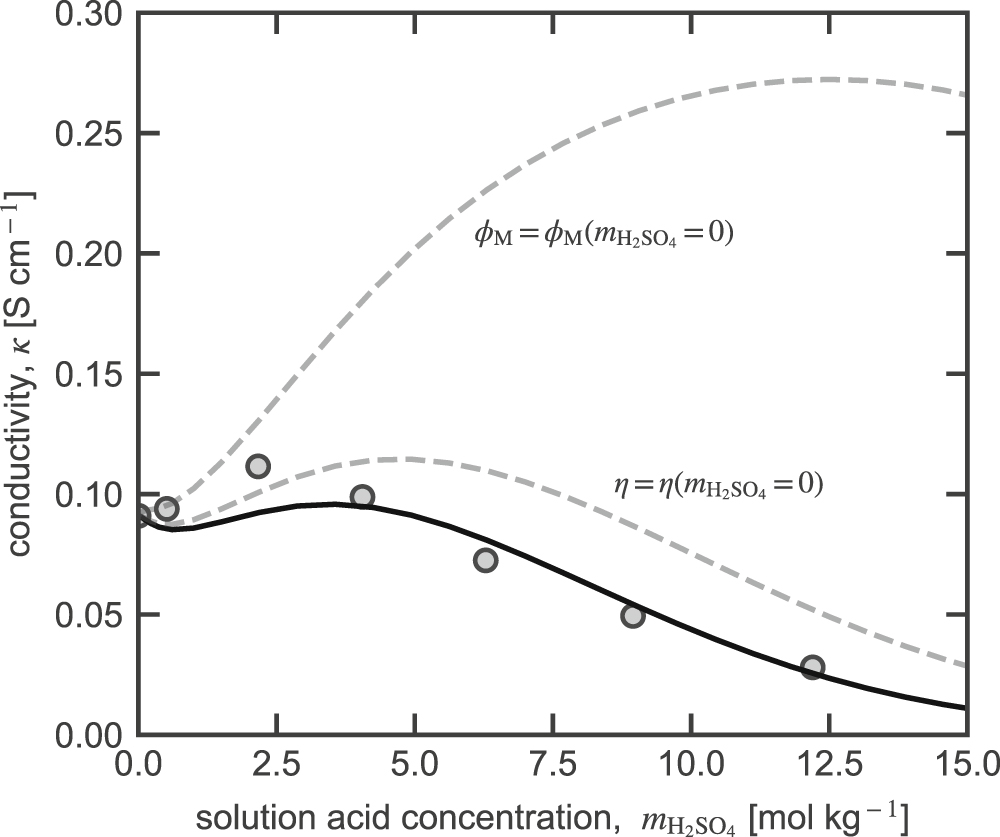
In concentrated electrolyte solutions, membrane water content and ion concentration induce large changes in transport properties. Part I⁴³ shows that membrane water content decreases and acid uptake increases with increasing bulk electrolyte concentration. Figure 4 shows measured^65,66 (circles) and calculated (solid line) N117 membrane conductivity as a function of external sulfuric acid concentration. Conductivity increases slightly up to a bulk electrolyte concentration of 4 mol kg⁻¹. At higher concentrations, conductivity decreases with increasing electrolyte concentration.

Zoom In Zoom Out Reset image size

Dashed lines in Fig. 4 show conductivity (hypothetical) if the viscosity of the electrolyte solution in the membrane $\eta$ or the membrane volume fraction ${\phi }_{{\rm{M}}}$ is equal to that of the membrane in acid-free liquid water (i.e., $\eta =\eta \left({m}_{{{\rm{H}}}_{2}{{\rm{SO}}}_{4}}=0\right)$ or ${\phi }_{{\rm{M}}}={\phi }_{{\rm{M}}}({m}_{{{\rm{H}}}_{2}{{\rm{SO}}}_{4}}=0),$ respectively). When viscosity of the electrolyte solution in the membrane is constant, membrane conductivity does not decrease as significantly at higher acid concentrations because proton mobility would be larger. When ${\phi }_{{\rm{M}}}$ is held constant, the conductivity increases as the acid concentration in the membrane increases. In actuality, as bulk acid concentration increases, membrane water content decreases (see Part I⁴³) causing increased tortuosity and decreased pore size. In agreement with Tang et al.⁶⁵, the delicate balance between decreasing proton mobility and increased number of charge carriers leads to a maximum in membrane conductivity at moderate acid concentrations.

Figure 5 plots calculated (solid line) and measured⁶⁷ (symbols) membrane conductivity as a function of either vanadium III, IV or V concentration with sulfuric acid such that the total sulfate concentrations is 5 mol dm^-3. The conductivity is normalized to the conductivity of the membrane in vanadium-free sulfuric acid to reduce propagation of error (see Fig. 4). Based on the proposed model for intermolecular friction, there is no friction between like-charged ions (see Eq. 12). Consequently, vanadium ions and protons do not directly interact at the microscopic description of the model (i.e. ${{\mathfrak{D}}}_{{{\rm{H}}}^{+}{{\rm{V}}}^{n+}(x)}^{{\rm{mol}}}=\infty$), but the presence of one still influences the other macroscopically (see Eq. 18). Although the current is carried mainly by mainly protons (dotted line shows this by plotting conductivity multiplied by proton transference number, $\kappa {t}_{{{\rm{H}}}^{+}}^{{\rm{M}}}$), as more vanadium is added to the membrane, the number of very mobile protons decreases and conductivity decreases. As Fig. 5 shows, the triply-charged V(III) displaces more protons and predicted conductivity curves are convex, whereas the singularly-charged V(V) curve is concave.

Zoom In Zoom Out Reset image size

In addition to conductivity and proton transference number, an array of other transport properties dictate multi-ion transport in ionomer membranes. Specifically, Figure S2 shows calculated vanadium transference numbers, electroosmotic coefficients, and ${\alpha }_{ij}^{{\rm{M}}}$ transport coefficients of Nafion in the same electrolytes as Fig. 5. Most of the transport properties are highly concentration dependent, and are starkly different between vanadium species. Although conductivity measurements, such as those in Fig. 5, are crucial to understand transport in these membrane, this single transport property provides a limited view of the diverse processes involved in transport.^2,63,67,78 Furthermore, dilute-solution descriptions that consider only one transport parameter for each species provide an incomplete understanding of transport in many instances. As Fig. S2 demonstrates, the proposed concentrated-solution model facilitates complete specification of transport properties of multicomponent systems using only two microscale, adjustable parameters, $\chi$ and $G.$