
Abstract
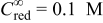
The behavior of semiconductor-based, light-activated microelectrodes in redox electrolytes has been examined theoretically using commercial software to self-consistently solve the transport equations for solid-state and solution-phase species and the electrostatic potential within the semiconductor phase, subject to the appropriate boundary conditions under steady state. The light-limited currents for such spatially localized microelectrodes, observed for a high voltage bias,  , under normal irradiation and a strict axisymmetric geometry, were proportional to the photon flux intensity. The results of these simulations afforded strong evidence that under high
 , holes generated by the light on an n-type semiconductor escape beyond the edge of the illuminated disk, leading to a net increase in the predicted current and thus in the effective area of the light-activated microelectrode.
Miller and Rosamilia1 described the use of a focused laser impinging at normal incidence on the surface of a semiconductor electrode immersed in an electrolyte containing a redox species to generate spatially localized currents with several possible applications.2 The implementation of this novel concept employing n-InP and n-GaAs disks in solutions of ferrocene (Fc) in well-supported acetonitrile electrolytes at high positive potentials,  , yielded a behavior closely resembling that of the conventional metallic microelectrodes.2, 3 This article seeks to theoretically examine certain aspects of such light-activated microelectrodes. A particular concern is to establish, under steady-state conditions and large
 , the influence of hole transport within the semiconductor beyond the illuminated area on the measured current, explicitly accounting for interfacial redox processes and mass transport of redox species in the solution phase.4
Theoretical Aspects
The system to be analyzed in this work involves an n-type InP semiconductor disk immersed in a Fc solution in a well-supported (1 M tetrabutylammonium tetrafluoroborate) acetonitrile electrolyte under conditions similar to those reported by Miller and Rosamilia.1 More specifically, we seek steady-state solutions for the transport equations for electrons (n) and holes (p), including both generation and recombination of n–p pairs,5, 6 self-consistently coupled to Poisson’s equation for the electrostatic potential within the semiconductor, φ, and to the transport equations for the donor [red (reduction)] and the acceptor [ox (oxidation)] species in a quiescent solution phase subject to the appropriate boundary conditions. The latter includes second-order kinetics7, 8 to account for the interfacial reactions between p (in the valence band) and red and between n (in the conduction band) and ox, which, for the parameters selected for this study, may be regarded as the dominant contributions to the measured current. A similar problem involving the partial illumination of a semiconductor without taking into account the mass transport from species in the solution phase was reported earlier by Mannheim and co-workers9 within the context of photocorrosion.
For these preliminary calculations, the Gaussian character of the laser intensity normal to the direction of propagation was ignored. Instead, the beam was regarded as a perfectly homogeneous cylinder of a radius,  , and thus smaller than that of the semiconductor disk of a radius,
 , impinging at normal incidence on the center of the n-InP disk so as to achieve strict axisymmetric conditions. The photon flux intensity of this beam is denoted as Φ. Schematic diagrams of the system in both three-dimensional (3D) (left) and cross-sectional views (right) are given in Fig. 1, where the magnitude of the illuminated area has been greatly enlarged (compared to the size of the semiconductor) for clarity. The overall approach implemented in this study follows rather closely that available in the TOSCA program,10 except that in the present case, the semiconductor was only partially illuminated and mass transport of species within the electrolyte was explicitly accounted for. Not considered in this brief study, however, were processes associated with the possible presence of surface traps, as well as the dependence of carrier mobility on the local electric field within the semiconductor.
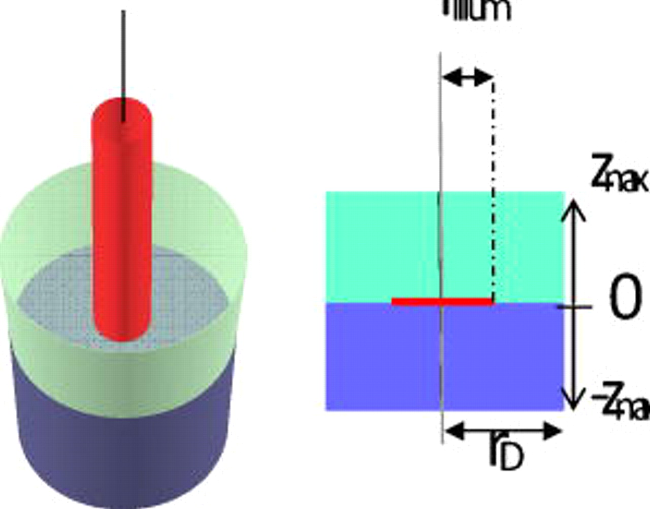
Figure 1. Schematic diagram on a light-activated microelectrode in both 3D (left) and cross-sectional views (right). The thin cylinder represents a homogeneous beam of light traveling through the transparent electrolyte phase (light cylinder above) impinging at normal incidence on the center of the semiconductor (dark cylinder below). The illuminated area has been greatly enlarged (compared to the size of the semiconductor) for clarity.
The governing differential equations within the semiconductor and electrolyte phases, including the boundary conditions, are given in Table I. For these simulations, the values of the relevant physical constants were obtained from either the literature10, 11 or prescribed by the characteristics of the semiconductor. Specifically, for n-InP, the direct recombination coefficient  , the absorption coefficient at
 ,
 , electron and hole mobilities
 and
 , which can be used to determine the corresponding electron and hole diffusivities from the Einstein relation, the bulk electron and hole concentrations
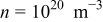 and
 , respectively, an intrinsic concentration of carriers
 , and a value for the donor density,
 . As in Ref. 1, the bulk concentrations of Fc and
 ,
 and
 , were set at 0.1 and 0 M, respectively. The diffusion coefficients of Fc and
 were assumed to be equal, i.e.,
 . Other parameters, such as the magnitudes of the second-order, potential independent rate constants7 for reactions between n and ox
 and between p and red
 , were adjusted to obtain values for the currents in line with those in the literature1, 10 (see the caption of Fig. 3). All calculations were performed within the COMSOL platform by meshing the domains with Lagrange triangular quadratic elements. As a means of validation, the global and local mesh sizes were increased until further refinements yielded no appreciable changes in the results (see the Appendix
Table I. Governing differential equations and boundary conditions associated with the theoretical analysis of light-activated microelectrodes.
| Semiconductor | Electrolyte solution | Equation |
|---|---|---|
| Governing differential equations | ||

| I.1 | |

|

| I.2 |

|

| I.3 |
| Boundary conditions | ||

| I.4 | |

| I.5 | |

|

| I.6 |

|
  
| I.7 |
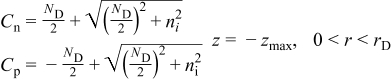
|

| I.8 |
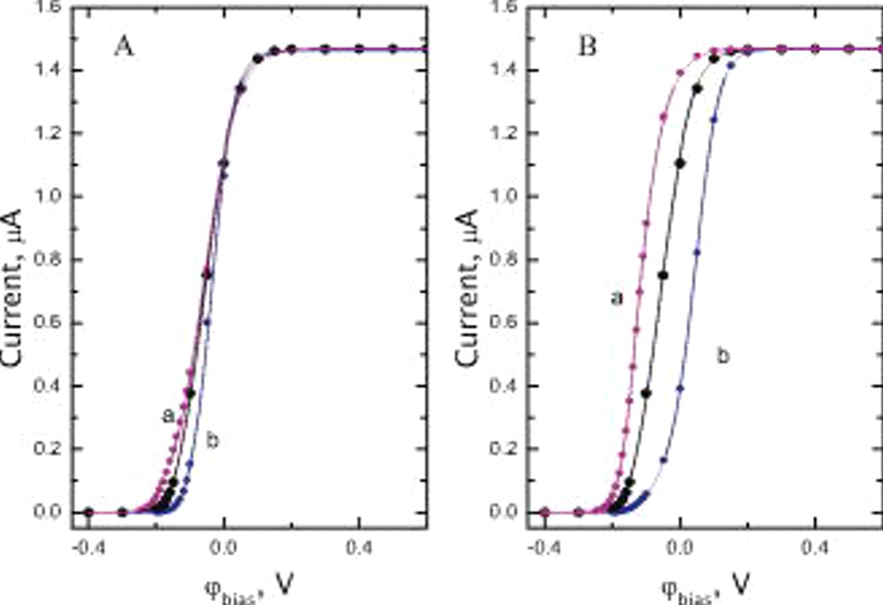
Figure 3. (A) Simulated polarization curve for an n-InP electrode in 0.1 M Fc in acetonitrile as a function of the value of the second-order rate constant for the reduction,  (curve a),
 (large symbols), and
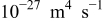 (curve b), assuming a constant second-order rate constant for oxidation,
 , of
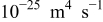 under illumination with a photon flux intensity of
 . The radius of the illuminated disk is
 . (B) Same as (A) as a function of the values of
 (curve a),
 (large symbols), and
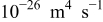 (curve b), assuming
 .
Results and Discussion
Shown in Fig. 2A is a polarization curve, i.e., current vs voltage bias, 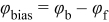 , where
 and
 represent the potential of the surface of the direct bandgap semiconductor (n-InP) in contact with the electrolyte and that of the ohmically contacted back face, respectively, under illumination (
 ,
 , see Fig. 1) by a homogeneous beam of radius
 . As indicated, the current is very small for small
 and becomes larger as
 is increased, reaching a sufficiently high bias, a limiting value independent of
 .
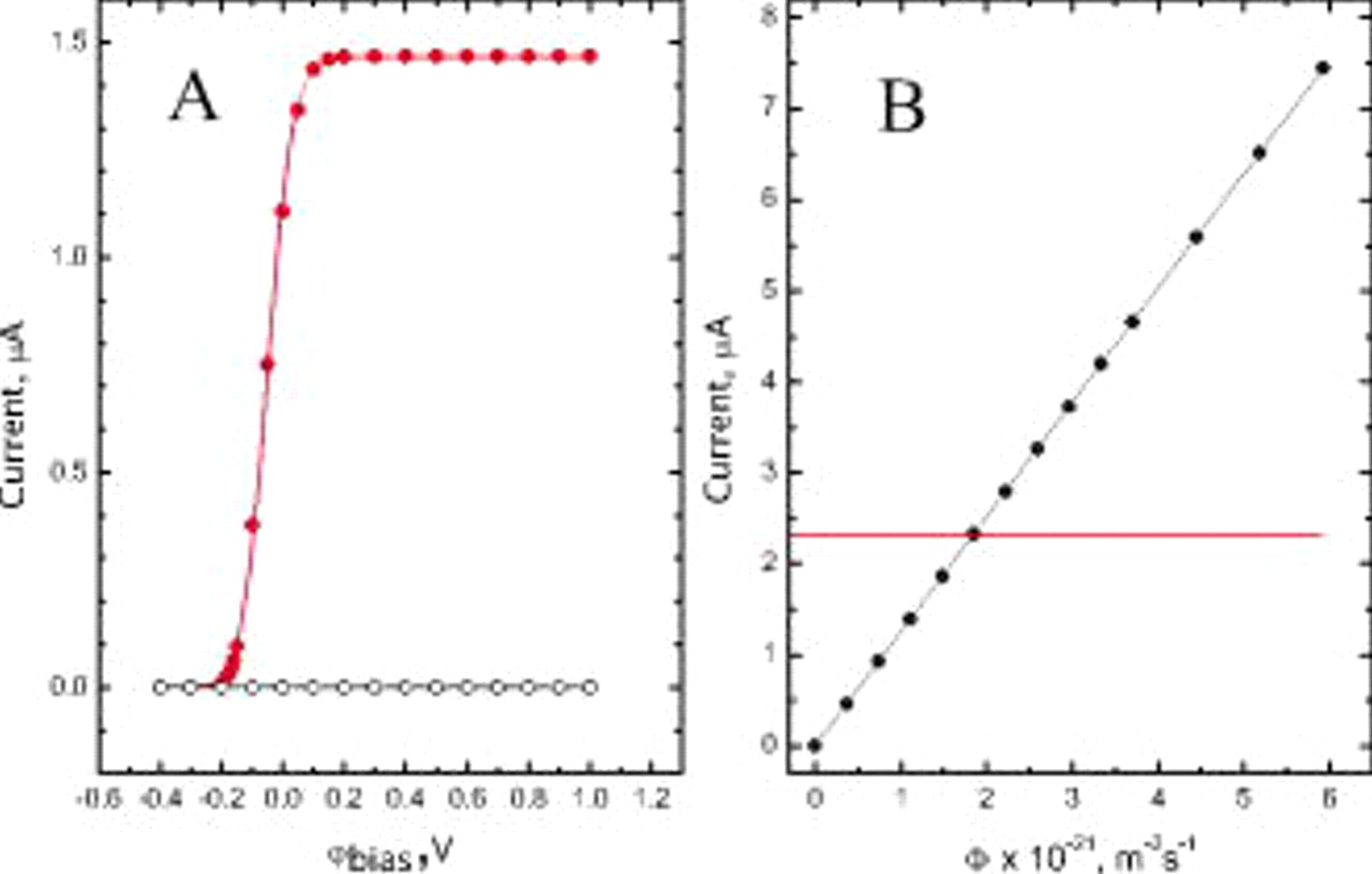
Figure 2. (A) Simulated polarization curve for an n-InP electrode in 0.1 M Fc in acetonitrile in the dark (open circles) and under illumination with a photon flux intensity of  (solid circles). The radius of the illuminated disk is
 (see Fig. 1 and text for details). (B) Plot of the total current as a function of the light intensity for
 . The solid line represents the best linear fit to the data (slope: 1.257, standard error
 , and intercept:
 ,
 ,
 ), whereas the dotted line parallel to the abscissa corresponds to the diffusion-limited current for Fc oxidation on a metallic microelectrode with a radius of
 , i.e.,
 .
In an analogy with the behavior of a uniformly illuminated semiconductor electrode and confirmed in our laboratory for spatially localized, light-activated n-InP microelectrodes for Fc solutions in acetonitrile electrolytes, the predicted current in this limiting region was proportional to Φ, the photon flux intensity (see Fig. 2B, for  ). Also shown in this figure (see dotted line) is the value of the diffusion-limited current,
 , for Fc oxidation on a metallic microelectrode of a radius,
 , for which
 . Thus, it follows from this plot that for
 , the light-activated electrode yields a current in excess of
 for a metallic microelectrode of the same radius. This provides strong evidence that a fraction of the measured current originates from areas of the electrode that are not being illuminated. Even for the highest Φ shown in this figure, i.e.,
 , the calculated surface concentration of red at the center of the disk, although small (3.3 mM), is not zero. This means that the limiting current from the viewpoint of the diffusion of the solution-phase reactant has not yet been achieved. The data shown in Fig. 3 illustrate the effects of the magnitudes of the second-order rate constants for the oxidation
 and reduction
 under otherwise identical conditions as those employed for the results shown in Fig. 2A (which are also given in large symbols in Fig. 3A and 3B). Curves a and b in Fig. 3A were obtained for values of
 (curve a) and
 (curve b) assuming
 , whereas those in Fig. 3B correspond to
 values of
 (curve a) and
 (curve b) for
 . As may have been expected, changes in these parameters elicit variations in the shape of the polarization curves for the small bias without affecting the values of the limiting current.
Color graded [panel (A)] and line contour plots [panel (B)] of the concentration of p and red,  and
 within the semiconductor and solution phases, respectively, determined for
 , well within the light-limited current range, and
 , are given in Fig. 4. Panels
 and
 in this figure are expanded views of panels (A) and (B), which highlight the features of dimensions comparable to the illuminated region, where the vertical line has been drawn at
 . The corresponding plots of
 can be simply obtained by subtracting the bulk concentration of
 and
 from the values of
 shown in the upper subpanels in panels (A) and
 . As evidenced above, as the interface is reached from the bulk of the semiconductor,
 increases, and from the bulk of the solution,
 decreases. The concentration of holes at the interface extends well beyond the edge of the illuminated area, i.e.,
 [see the dotted line in panels
 and
 , Fig. 4].
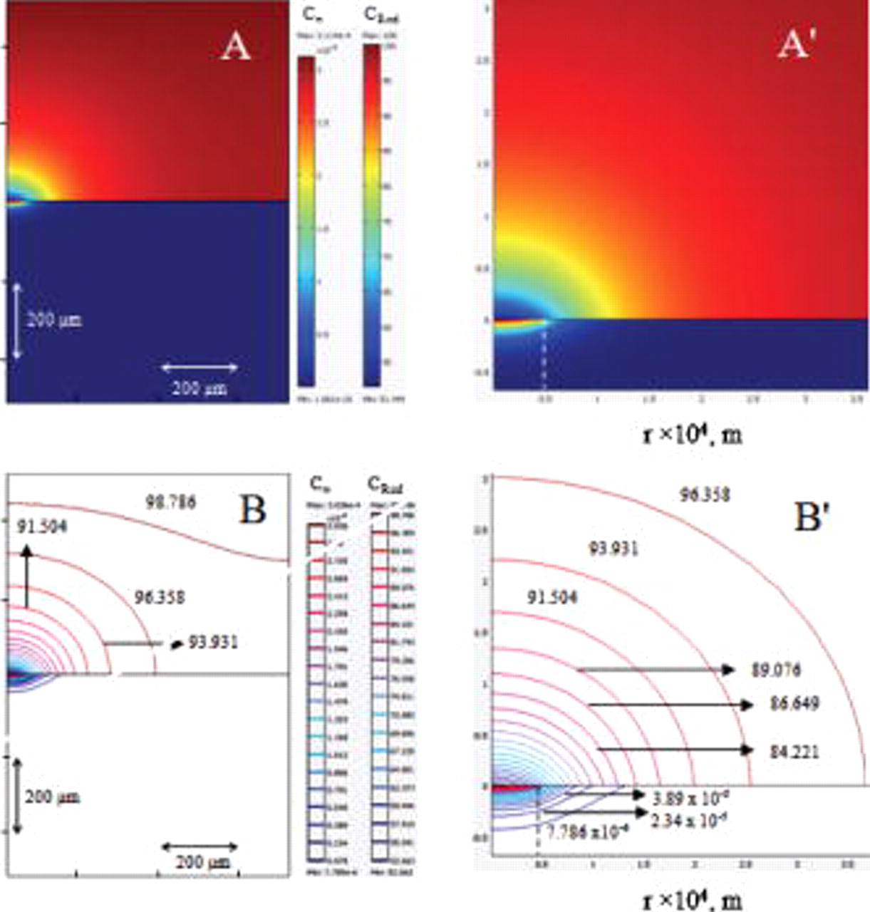
Figure 4. (A) Color graded and (B) line contour plots of  (in
 , upper subpanels) and
 (in
 , lower subpanels) for
 and
 .
 and
 are expanded views of
 and
 based on the lower subpanels in (A) and (B), respectively. The dotted vertical lines represent the edge of the illuminated area.
The local current flowing across the semiconductor/solution interface can be related to the concentrations of n, p,  , and
 at the interface through the quantity
 , where the first and second terms account for the reduction and oxidation currents at the interface or to the flux of either one of the two redox species in the solution. Shown in Fig. 5 in thin lines (lower abscissa) are plots of
 (in
 , black curve, left ordinate) and
 (in nmol
 , gray curve, right ordinate) and of
 (upper curve) and
 (lower curve, panel B) for n-InP. The thick lines in panel (A) represent the same data in an amplified
 axis (upper abscissa) for clarity, where the dotted vertical line at
 represents the edge of the illuminated region. In fact, based on the values of the rate constants selected for this preliminary study, the contribution to the total current due to the reduction reaction is indeed negligible. A calculation of the current based on
 yielded the same values as those evaluated from the flux of red at the interface,
 , along the radial direction, given in thin black lines in Fig. 6A (lower abscissa). Also given in this panel in thick lines are the same data over a smaller range in an expanded scale (see upper abscissa). As clearly evidenced from these results,
 only decays to the negligible values at distances beyond the light illuminated edge, indicating that the contribution to the total current due to the nonilluminated area is indeed significant. This aspect is best illustrated by a plot of the fractional current as a function of
 ,
 , in Fig. 6B, defined as
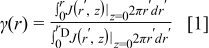
which represents the ratio of the current of a disk with radius  normalized by the current over the entire n-InP disk, i.e.,
 (thin black line, upper abscissa). The same data in an expanded scale (lower abscissa) are given by the thick black line in the same panel in this figure. On this basis and for the parameters selected for this simulation, the fraction of the current flowing through the illuminated area,
 , i.e.,
 , amounts to 42%, i.e., less than half the total current. It may be surmised from these considerations that for a semiconductor displaying a smaller absorption coefficient, the light would penetrate deeper into the material generating n-p pairs farther away from the surface, thus allowing for the holes to reach distances longer than those found for n-InP. This was the case for n-Si (see gray curves in Fig. 6A and 6B), an indirect band semiconductor, for which the absorption coefficient at
 is
 ,
 ,
 ,
 , and
 , and the lifetimes of electrons and holes
 and
 are equal to
 . For n-Si, the recombination rate was assumed to be given by the Shockley–Read–Hall (SRH) equation,12, 13
 by regarding the trap level to be located in the middle of the bandgap, meaning that the concentrations of the electrons and holes in the trap level equal
 . As shown in Fig. 6B,
 for n-Si is only 27%.
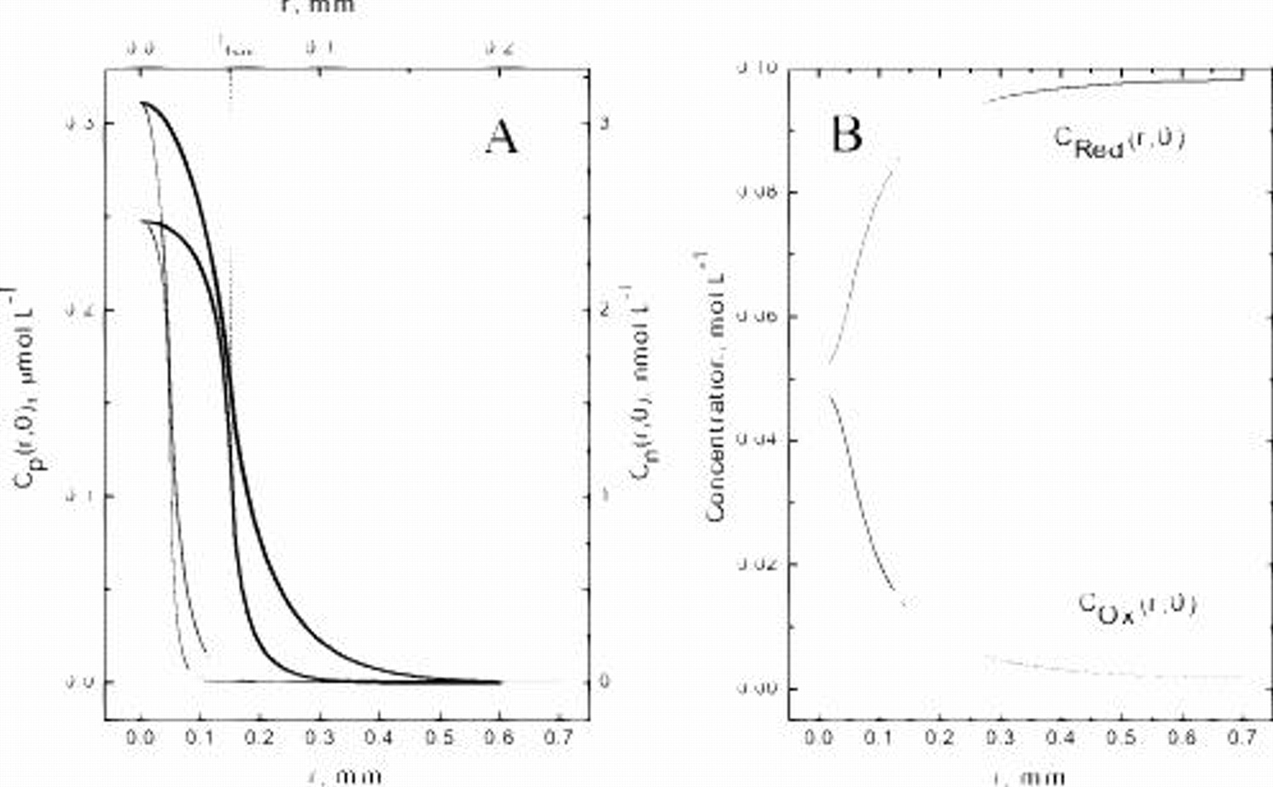
Figure 5. A. Plots of  (left ordinate, thin black curve) and
 (right ordinate, thin gray curve) as a function of
 along the semiconductor–solution interface for otherwise the same system described in Fig. 4. Note the difference between the scales for the two carriers. The thick curves represent the same data in an expanded
 scale (see upper abscissa). (B) Plots of
 (gray, upper trace) and
 (black, lower trace) as a function of
 along the interface. The dotted vertical line at
 (see upper abscissa, left panel) represents the edge of the illuminated region.
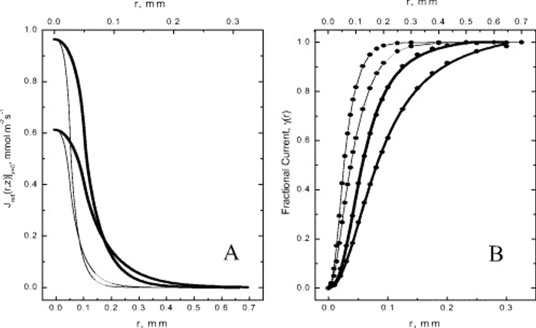
Figure 6. (A) Plot of the normal flux of  across the
 interface,
 , as a function of
 for n-InP (thin black line) and n-Si (thin gray line) for otherwise the same system described in Fig. 4. The same data in an expanded
 -scale (upper abscissa) are shown by the corresponding thick lines. (B) Plots of the radial dependence of the fractional current, γ, for n-InP (thin black line) and n-Si (thin gray lines, see upper abscissa). The same data in an expanded
 -scale are shown by the corresponding thick lines in this figure (lower abscissa).
List of Symbols

| direct recombination coefficient |

| bulk concentration of ox |

| bulk concentration of red |

| electron diffusivity |

| diffusion coefficient of ox |

| hole diffusivity |

| diffusion coefficient of red |

| second-order rate constant for reduction |

| second-order rate constant for oxidation |
| n | bulk electron concentration |

| intrinsic concentration of carriers |

| acceptor dopant density |

| donor dopant density |
| p | bulk hole concentration |
Greek
| α | absorption coefficient |

| electron mobility |

| hole mobility |

| lifetime of electrons |

| lifetime of holes |
| Φ | photon flux intensity |
Acknowledgments
Support for this work was provided by a grant from the NSF. Fruitful discussions with Professor Stanley Bruckenstein are deeply appreciated.
Case Western Reserve University assisted in meeting the publication costs of this article.
:
Appendix
A schematic diagram of the domains defined in the simulations is shown in the left panel, Fig. A-1, where the upper (gray) and lower (white) regions represent, respectively, the solution and semiconductor phases. The global predefined mesh is finer (see right panel). For boundary 4 (the illuminated region at the interface, i.e.,  ), the maximum element size was
 and the element growth rate
 ; for boundary 6 (nonilluminated interfacial region,
 ), the maximum
 and
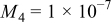
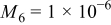
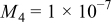
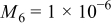
 . There are a total of 70,792 elements in the space. To assess the validity of the results, the mesh size was increased until the differences in the calculated results were very small. An example involving the total current is given in Table II.
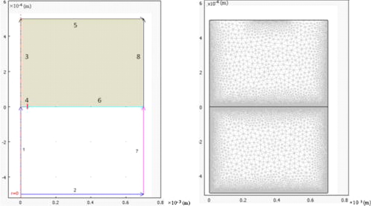
Figure 7. Definition of the boundaries, domains (left), and mesh (right) as implemented in COMSOL.
Table II. Integral of the flux along boundaries 4  and 6
 in
 for two different global mesh values
 for a fixed mesh value for boundary 6
 using finer mesh values for boundary 4
 , total current
 , and difference between the results of the mesh size for
 ,
 ,
 ,
 ,
 , and photon flux intensity
 . The data in the middle row specify the conditions employed in this article.
 
|
 
| Total current  
| Difference (%) | |
|---|---|---|---|---|
| 0.62503 | 0.83826 | 1.46329 | 0.37 |

| ||||
| 0.62638 | 0.84241 | 1.46879 | — |
| ||||
| ||||

| 0.62638 | 0.84222 | 1.4686 | 0.013 |
| ||||
|