
Abstract
The primary and secondary current distributions for the particle incorporation process during electrocodeposition of a metal film were numerically studied. The growth of an electrodeposited film along the electrode is governed by the local current density that is affected by the presence of a nonconducting particle. It was assumed that the effect of lateral displacement of the fluid between a particle and an electrode is negligible. The level set method was used to track the moving interface as it grows around the particle, and the Laplace equation for the electrical potential was solved by a finite-element method. For a primary current distribution, voids beneath the particle are generated due to the characteristics of the potential distribution, so that the metallic film does not grow along the particle surface. The resistance increment due to the presence of the particle was compared for the cases of stationary and growing metallic films. A small void on top of the particle when incorporated by metal is observed with a secondary current distribution.
Metallic matrix composite films are produced by occlusion of particles during electroplating. This process for making composite films has many advantages in industrial applications due to the uniformity of deposition, even for complex shapes, and the avoidance of high-temperature and high-pressure processing.1 Electrocodeposition is a function of many process variables, such as bath composition, hydrodynamics, current density, particle characteristics, and so on. Bath composition encompasses the concentration and type of electrolyte, particle loading in suspension, pH, temperature, and additives. Our experimental research to date has been primarily focused on electrocodeposition under controlled hydrodynamics using a rotating cylinder electrode2 or impinging jet as a function of process variables, such as current density and bath composition, for copper-alumina composites. However, the physical phenomenon of electrocodeposition is not well understood.3
The general mechanism of electrocodeposition is as follows: (i) a particle suspended in bulk solution is transported to the neighborhood of the electrode surface by the forced convection of the electrolyte, (ii) particles come into contact with the electrode surface, (iii) particles either stay adsorbed or detach from the surface, and (iv) particles adsorbed on the surface are captured by the growing metal film. The hydrodynamics in electrocodeposition play a significant role for the transport of ions and particles. Various mechanisms can contribute to the transport of particles to the electrode: Brownian diffusion, hydrodynamic convection, electromigration, and diffusiomigration.
Guglielmi proposed the first model for electrocodeposition which was a two-adsorption step process in 1972.4 The proposed steps were (i) to produce a layer of loosely adsorbed particles and then (ii) a strong adsorption of the particles onto the electrode. Celis et al.5 assumed that a particle will only be incorporated into the metal film when a certain amount of the adsorbed ions on the particle surface is reduced. A statistical approach was taken to give a quantitative description of the incorporation of an inert particle into a growing metallic matrix. Valdes6 developed a model for the deposition of colloidal particles onto a rotating disk electrode (RDE). An equation of continuity was derived for the particle number concentration where the particle flux consists of a diffusion term governed by Brownian motion and a convection term governed by the convective velocity driven by the hydrodynamic convective velocity, electromigration, diffusiomigration, and any specific forces of interaction. The convective diffusion equation was solved with a boundary condition in which an electrochemical reduction of electroactive ions adsorbed on the particle provided the essential surface binding interaction that was responsible for particle deposition. The model predicted that the rate of particle incorporation increased with increasing current density, reached a maximum value, and decreased for larger current densities. Fransaer et al. ,7 using an RDE, explained the electrolytic codeposition of non-Brownian particles based on a trajectory analysis coupled to a surface immobilization reaction. They assumed creeping flow motion for the fluid and decomposed the local flow into an axisymmetrical stagnation flow, two linear shear flows, one parabolic shear flow, and a local rotation. Taking a force balance on the sphere, the trajectory equations were derived for a particle near an RDE in terms of forces acting on a particle. Here the external forces were derived by considering long-range forces, dispersion forces, double-layer forces, and concentration and potential fields. As a boundary condition, the behavior of particles in the vicinity of the disk was formulated by two reaction terms for the particle immobilization and the removal rate, respectively. Using this concept, they avoided the usually applied perfect sink condition. To obtain the flux of particles to the disk, the instantaneous probability was introduced in which a particle remains on the electrode in terms of the forces immobilizing the particle and the removal force. However, the trajectory model did not consider the growth behavior of the metal deposit. Adamczyk and co-workers8, 9 examined the kinetics of localized adsorption of colloidal particles at collectors having a flow stagnation point such as a rotating disk, impinging jet, and a sphere or cylinder in uniform flow. The filtration-type model was developed based on two approaches.10 The first one was the Lagrangian method which considered the trajectories of individual particles in the flowing fluid using Newton’s Second Law. Usually this approach is applied for non-Brownian particles. The second was the Eulerian method, which was a statistical approach for Brownian particles. It described the particles collectively in terms of their distribution function. However, there has not been a study to show the entire entrapment process, even with only a primary current distribution. The objective of this study is to simulate the incorporation of a particle by the growing metal film for primary and secondary current distributions in a stationary fluid.
Newman11 and West and Newman12 gave the fundamental principles for developing the primary and secondary current distributions with the Laplace equation. They presented the various techniques such as coordinate or similarity transformations, potential theory, boundary integral technique, and perturbation theory. Dukovic13 reviewed the computation of current distributions in electrodeposition, particularly focused on the electronics industry, giving many references for numerical methods such as the finite-difference method (FDM), the finite-element method (FEM), and the boundary element method (BEM). The current distribution studies were classified into four size scales: workpiece, pattern, feature, and roughness scales. An integral equation approach was utilized to analyze the current density distribution at a disk-shaped microelectrode at steady state,14 where the result was compared with an asymptotic approximation. An electrochemical system governed by diffusion, convection, and migration was studied by Qiu et al.15 using the boundary element method, where examples were shown for parallel plate electrodes with a laminar flow. However, the studies have concentrated on current density distributions on electrodes and in the electrolyte without a particle. To the authors’ knowledge, there is no study related to the moving electrodeposited film occluding a particle.
With primary and secondary current distributions, the electrical potential is governed by the Laplace equation. To study the primary current distribution around an insulating sphere above a plane, the bispherical coordinate is a good choice. The general solution procedure for the Laplace equation using bispherical coordinates for two spheres was studied in detail by Stoy for parallel16 and perpendicular17 orientations in a uniform external field. The potential field around an insulating sphere normal to a conducting plane was obtained by Morrison and Stukel.18 They also considered the axisymmetric viscous flow with an assumption of Stokes flow and derived the correction of the electrophoretic velocity in the presence of a conducting wall.
The tangent sphere coordinate has been used to obtain a solution for the electrical potential around a particle contacted on a plane. Sides and Tobias19 obtained the analytical solution for the potential field around a bubble on a plane electrode, where a bubble can be regarded as an insulating sphere. The potential was composed of two contributions: one was the linear term which satisfied the field in the absence of the bubble, and the other was the disturbance term which was perturbed by the presence of the bubble. The potential was obtained by matching the insulating boundary condition on the bubble surface and then the primary current distribution on the electrode was given by the normal derivative of the potential on the plane. They reported the resistance increment caused by the bubble, and extended the solution to the resistance increment of surface layers of ordered dielectric spheres and the increment given by spheres dispersed in bulk electrolyte.20 Fransaer et al.21, 22 considered the Laplace equation for a conducting or an insulating sphere on either a conducting or an insulating surface, where the complete solutions were expressed in terms of series expansions instead of integral solutions. They showed the resistance increment of ordered and random arrays of particles from a net effect of a single particle and compared the resistance variation on a conducting plane of a conducting particle with that of a nonconducting particle by Sides and Tobias.19 Finally, they also investigated the Laplace equation around a spherical ridge or trough in a plane in toroidal coordinates.23
For multiphase flow simulation, an interface can be considered as a boundary that divides the phases. The immersed boundary method which uses a finite-difference mesh in which the boundary evolves following the equation of motion, has been used to simulate a moving interface.24 Two numerical approaches to deal with the interface are the front-tracking method and the front-capturing method.
The front-tracking method discretizes the moving front into a set of marker points. The positions of the marker points are updated in time. The advantage is that the interface is explicitly tracked. This method can be accurate in a small deformation motion. However, for large and complex motion, it is not an appropriate approach, because there is an instability of the marker points. Marker particles representing the interface can come together or oscillates in local regions, where regridding and smoothing techniques are needed to avoid this instability. When two interfaces also merge together to form a single one, another technique is needed to eliminate parts of the boundary and to connect two boundaries into a new single one. Consequently, the computational cost is high to resolve these problems. The front tracking method was used to study the effects of surfactants on the deformation of drops and bubbles.25
The second approach is based on the front-capturing method. In a level set formulation defined on the entire domain, the boundary is modeled as the zero set of a smooth function. The boundary is then updated by solving a nonlinear equation of the Hamilton-Jacobi type on the whole domain and tracked implicitly. The advantages are that regridding and smoothing techniques are not needed and highly complicated boundaries can be represented easily. Therefore, the moving interface can develop sharp corners or edges in two- and three-dimensional problems.
If the time-dependent moving boundary by the zero level set  is in general considered,26, 27 the motion of the interface is represented by the chain rule

where  is the interface velocity,
 is the speed in the normal direction on the interface, and
 is a unit normal vector. Here,
 is the Hamiltonian. Since Eq. 1 is a hyperbolic equation, the characteristic direction depending on ψ is considered. Therefore, the main numerical idea of the level set equation is related to the numerical method of the hyperbolic equation and Hamilton-Jacobi equations.
Osher26 and Sethian27 introduced the level set formulation for the moving interface and formulated the evolution equation of an interface as a type of Hamilton-Jacobi equation. The key idea in a level set formulation is to represent the moving boundary as a particular level set implicitly in a way that sharp gradients and corners are easily expressed. The application for fluid interfaces was recently summarized by Sethian and Smereka.28 Adalsteinsson and Sethian29, 30 applied the level set approach to etching, deposition, and lithography processes in two- and three-dimensional simulations, where they used the fast level set method, considering only points close to the interface at every time step.31 Wheeler et al.32 used the level set method to investigate the superconformal electrodeposition for the void-free filling of a high aspect ratio geometry. Their contribution was to set up the surface coverage model for electroplating bath additive accumulation and conservation on a moving metallic interface with the level set method.
In this paper, the particle incorporation process in electrocodeposition is numerically considered with an assumption of no lateral displacement of the fluid between the particle and the electrode. The growth of an electrodeposited film along the electrode is controlled by the local current density affected by the presence of an insulating particle. One of the goals is to investigate the resistance variation in the presence of an inert particle. The electrical potential is obtained by solution of the Laplace equation with boundary conditions for both the primary and secondary current distributions. Then, the current density is computed from the normal potential gradient on the metallic interface. For the secondary current distribution, the surface overpotential is given by the Butler-Volmer equation and is used as a boundary condition on the metallic surface to obtain the potential field.
Formulation of a Particle Incorporation Model
Governing equations and boundary conditions
We consider the particle incorporation process during electrocodeposition for primary and secondary current distributions, where the concentration gradients in the electrolyte are negligible. The conductivity of the electrode is assumed to be infinite compared to that of the solution.33 Then, the metallic interface between an electrode and an electrolyte is an equipotential surface. The metallic interface is initially flat and grows proportional to the normal gradients of electrical potential fields that are affected by the presence of an insulating particle of radius  , as illustrated in Fig. 1, in which the physical configuration is defined on Cartesian coordinates,
 and
 .
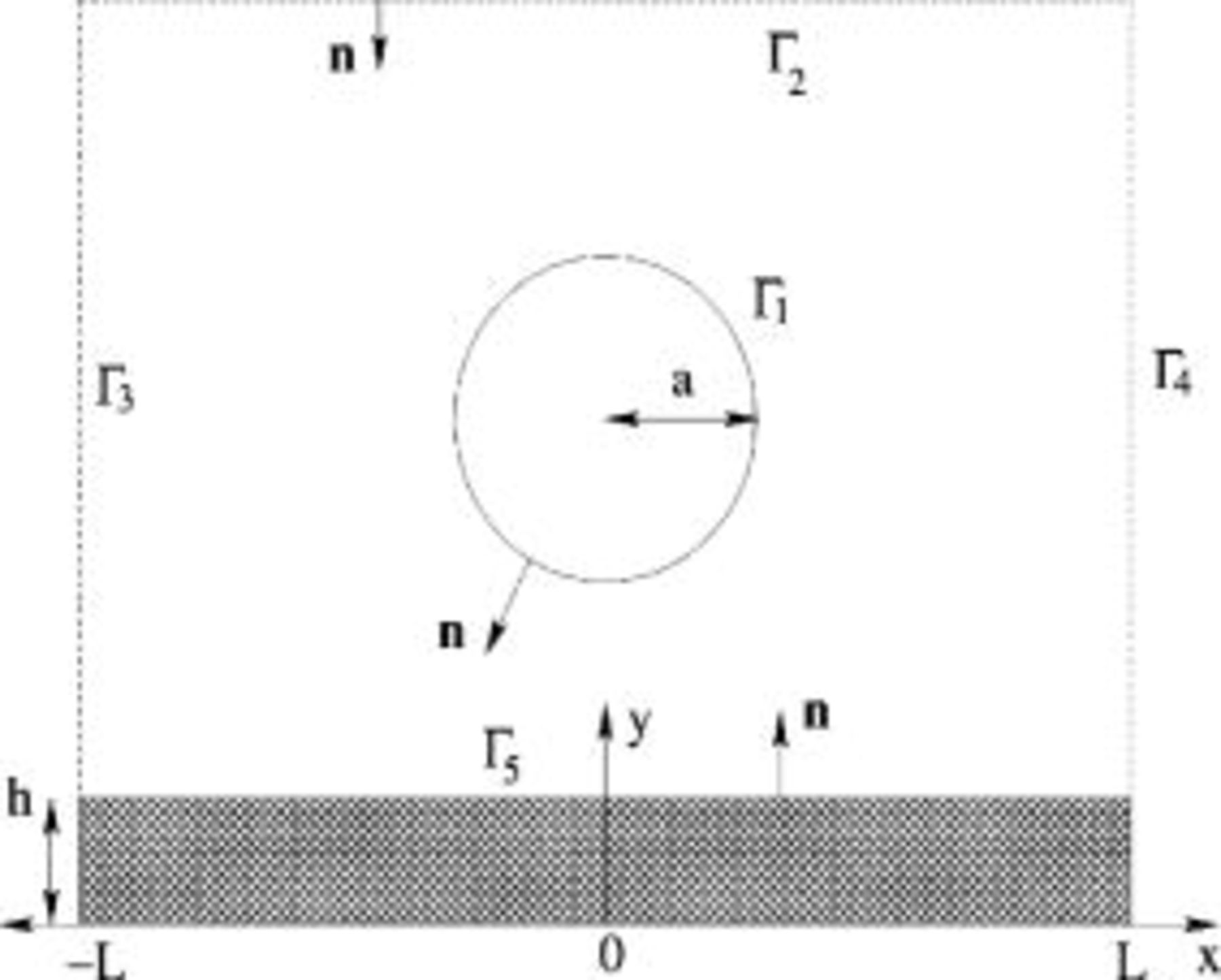
Figure 1. Physical configuration.
The molar flux of the  species in the absence of a concentration gradient is given by

where  is the mobility,
 is the charge number,
 is Faraday’s constant,
 is the gas constant,
 is the absolute temperature, and Φ is the electrical potential.33 We consider only the contribution of the flux due to migration in an electric field. The current density
 due to the movement of charged species is given by

where  is the electrical conductivity of the solution and ∑ denotes the summation over
 . Taking the divergence of Eq. 3 gives the Laplace equation for the electrical potential

Periodic boundary conditions are applied on  and
 , i.e.,
 , as shown in Fig. 1, and on the top boundary


where  is the average current density,
 is the unit normal vector pointing into an electrolyte solution,
 is the current density normal to the electrode surface, while on the surface of an uncharged particle


The evolution of the metal film on  is governed by the growth rate
 that is defined by the local current density normal to the surface

where  is deposited film thickness,
 is the molecular weight of the depositing species, and
 is the density of the cathodic deposit. Since the current at the cathode is negative, the metal film grows toward the electrolyte solution. For a primary current distribution, the electrical potential on the electrode surface
 is assumed to be zero

where  is the potential at the cathode surface. For a secondary current distribution, the total potential
 is given by

where  is the surface overpotential. The current density normal to the electrode is represented by the Butler-Volmer equation

where  is the exchange current density and
 and
 are the anodic and cathodic transfer coefficients, respectively. Since
 is set to zero and
 , the nonlinear boundary condition for the electrical potential Φ is derived as

By nondimensionalization of the variables [all lengths by the particle radius  , time by
 , growth rate by
 , current density by
 , and potential by
 ], two controlling parameters,
 and
 , are obtained, where
 and
 are the nondimensionalized average current density and exchange current density, respectively. Therefore, the nondimensionalized boundary condition on
 is
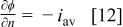
where ϕ is the dimensionless electrical potential, and on the surface of an uncharged particle 

On the electrode surface  , for the primary current distribution

while for the secondary current distribution

where the dimensionless exchange current density  . The evolution of the metal film thickness is obtained from Eq. 7, which in dimensionless form is
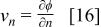
where  is the dimensionless growth speed, and equals the speed function
 in Eq. 1. The time scale τ will be used for the computation of the level set function ψ.
Motion of an insulating particle
The motion of an uncharged particle with a velocity  at steady state is given by

where  is the friction coefficient. The first term on the left-hand side of Eq. 17 is the frictional force, where β is the resistance of a single particle in Stokes flow and decreases to zero in the neighborhood of the wall by Brenner’s correction.34 The
 and
 terms represent the attractive van der Waals force and other external forces such as the gravity, buoyancy, or convectional motions, respectively. In this study, the force field
 is expressed in terms of the attractive van der Waals force between a sphere and a plane solid surface
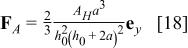
where  is the unit vector in the
 direction,
 is the Hamaker constant, and
 is the minimum distance between the particle and the flat electrode.35
When the particle is far away from the electrode, that is,  , the effect of the van der Waals force is negligible. Then, in a stationary fluid, the particle moves toward the electrode in the direction of negative
 with a terminal velocity
 due to the external forces
 . Even if the particle is accelerated because of the van der Waals force as the particle approaches the wall, it is assumed that the accelerated time is short enough that the particle moves with a constant velocity when it contacts the wall. On contacting the electrode, the rigid particle is strongly attached to the electrode due to the van der Waals force. Here, we neglect the lateral displacement of fluid induced by the particle motion toward the electrode.
Computational method
In electrocodeposition, there exist three phases: the particle, the deposited film, and the electrolyte, and interfaces between these phases. Additionally, the interface between the deposited metallic film and the electrolytic solution is a moving boundary by reduction of metallic ions. An efficient numerical method is then needed to track the growing surface. In this section, the level set method is introduced as a computational method to calculate the evolution of a growing metallic interface using Cartesian coordinates  shown in Fig. 1.
For instance, Fig. 2 shows the level set of  defined by
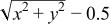 . Each level set indicates an isocontour line. A zero level set represents a circle of radius 0.5. Two regions are separated at a zero isocontour line:
 or
 . When
 in Eq. 1 is constant, each level set of
 propagates toward the outward normal direction with the same speed.
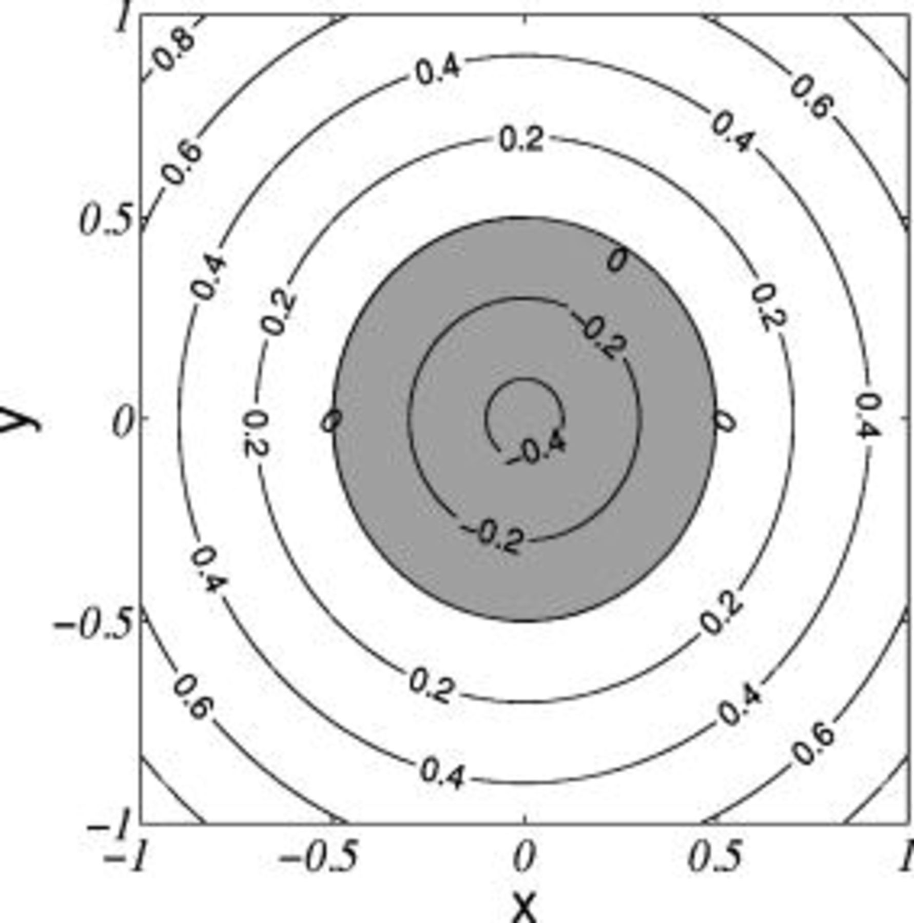
Figure 2. Level set of  .
In this study, three level set functions normalized by the particle radius  are introduced:
 for a particle,
 for the electrode interface, and
 for a combination of
 and




where  is the particle center position,
 is the initial position of the electrode, and
 and
 are components of the position vector
 . The initial metallic interface is represented by a line of
 , and a line of
 represents a moving metallic interface at each time step. As time goes on, the level set function is computed by Eq. 1, and the moving interface is tracked as follows

where  is substituted by
 defined by Eq. 16 and
 is normalized by τ. Because the speed
 is defined only on the interface and the level set function is defined on the finite-difference mesh of the whole domain, the extension of the speed function
 to the entire domain of a finite-difference mesh must be considered. The values of
 enclosed by boundaries Γ are easily computed on the computational domain. The problematic regions are inside the particle and beneath the moving metallic surface, because
 in the regions are not specified. In this study, the technique called impainting, which is used for restoration of degraded images in image processing, was used to extend
 .26 Accordingly, the values of
 inside the particle are found by solving the Laplace equation
 with the fixed values near boundary mesh points. For values of
 at the finite-difference mesh right beneath the metallic interface,
 is assumed; the coefficients
 ,
 , and
 are determined by solving the linear equations based on three known points above the metallic interface. The values right beneath the interface are then interpolated using the coefficients, and the same values are used for the finite-difference nodes to the bottom boundary in a vertical direction.
To improve the computational speed, fast level set techniques were introduced.36 The central idea of a fast level set implementation is to let the level set function ψ consider a signed distance function  26

where  is an interface position vector and a condition of
 is imposed. Note that
 on the boundary and its gradient is unity. The sign is plus and minus in regions where the level set function values are larger and smaller than zero, respectively. The fast sweeping method37, 38 is a nonlinear upwind difference and uses Gauss-Seidel iterations with alternating sweeping ordering in order to extend the signed distance function. The advantage is a simple numerical implementation. The accuracy is the same as other methods which solve the same system of discretized equations.37 The moving metallic interface is then tracked implicitly by the level set approach, which enables the simulation of the entrapment process around the nonconducting particle.
The PLTMG (Piecewise Linear Triangle Multi Grid Package) was used to solve the Laplace equation for the potential fields.39 This package is a finite-element solver for solving elliptic partial differential equations in a two-dimensional space and provided the continuous piecewise linear triangular finite elements and adaptive local mesh refinement. In this study, the coarse grids are first produced in the whole computational domain, and the fine meshes are created by the adaptive refinement algorithm by the error estimate.
The computation procedure is as follows: (a) finite-element grids are generated subject to boundary positions, (b) the potential ϕ at the finite-element nodes was obtained by PLTMG with corresponding boundary conditions, (c) the potential and the gradient of potential at each node in a finite-difference mesh were interpolated in the computational domain enclosed by boundaries Γ, (d) the normal components of the unit vector  at finite-difference nodes were computed by the level set function, (e) the speed function
 encompassed by Γ was obtained by the inner product of the vector and the gradient of potential at each node using previously computed solutions in (c) and (d), (f) the speed function
 inside the particle and beneath the electrode surface was impainted by values of
 close to
 and
 , (g) the moving interface was tracked implicitly by Eq. 22, (h) the level set function was recalculated by the fast sweeping technique, (i) using the basic property of the distance function, the interface position was interpolated and used for the boundary positions for PLTMG, and (j) the simulation was iterated until the process was completed. In this study, the finite-difference mesh size
 and time step
 were used (0.05 and 0.00625, respectively). The maximum number of refined triangles generated by PLTMG used was up to 1500. The maximum computational time using a Dell Precision 620 (1.0G Memory) computer was
 . The computational domain is defined on a grid size of
 by
 , where
 and
 , and the initial height of the metallic surface
 is set to 1.
Primary Current Distribution
The primary current density distribution depends only on the geometry of the system because the influence of overpotential is zero. Due to the infinite conductivity of a metallic electrode, the resistance of the electrolyte (ohmic drop) is comparatively much larger than the kinetic resistance due to the surface overpotential, therefore a primary current distribution is the limiting condition of negligible kinetic resistance. Thus, the potential is constant at the metallic interface. When we consider an insulating particle in contact with a conducting wall, the contact angle between the particle and the electrode causes a change of current density around the contact point; the current density will be infinite when the angle is obtuse and zero when the angle is acute. West and Newman40 investigated the current distribution near an electrode edge using a singular perturbation analysis and showed that the current density at the intersection point approaches extreme values as the primary distribution is approached. A change in current density affects the shape of the evolving surface, which may change the microstructure of the electrodeposited film.
Sides and Tobias19 calculated the resistance increment caused by bubbles attached to an electrode. Fransaer21, 22 investigated the resistance increment of insulating particles on a disk electrode to develop algorithms to determine the position of particles on the electrode. The analytical solution for electrical potential was obtained by a series expansion. In the region without the particle, all current density vectors are parallel to each other. However, the nonconducting particle acts as an obstacle that prevents the current from flowing to the electrode. Additional voltage is needed for the current density around the obstacle and this induces a resistance increment,  , which is the net voltage change divided by the average current density. In the absence of the particle, the potential field with a flat fixed metallic interface is analytically given by
 . The case with a growing metallic film will be discussed later. The potential field depends only on the
 direction normal to the metallic substrate. The voltage difference is obtained by subtracting
 from the computed average potential in the presence of the particle on the top boundary
 . The resistance increment as a function of
 , which is the minimum distance between the electrode and the particle and is normalized by the particle radius
 , is represented in Fig. 3. After one radius distance away from the interface, the voltage increment stays constant. This means that the current flow is not affected by the presence of the electrode. As the particle approaches the electrode, the resistance increment decreases and converges to a nonzero value. When the particle is incorporated completely by the growing metallic film, the resistance increment will be reduced to zero because of no further voltage increment due to the presence of the particle. As
 increases, the effect of the particle becomes less because the area ratio of the particle in the domain is reduced. The resistance increment changes noticeably as the spacing between particles becomes smaller.41 The results by Sides and Tobias19 for a single bubble on an electrode are also shown in Fig. 3.
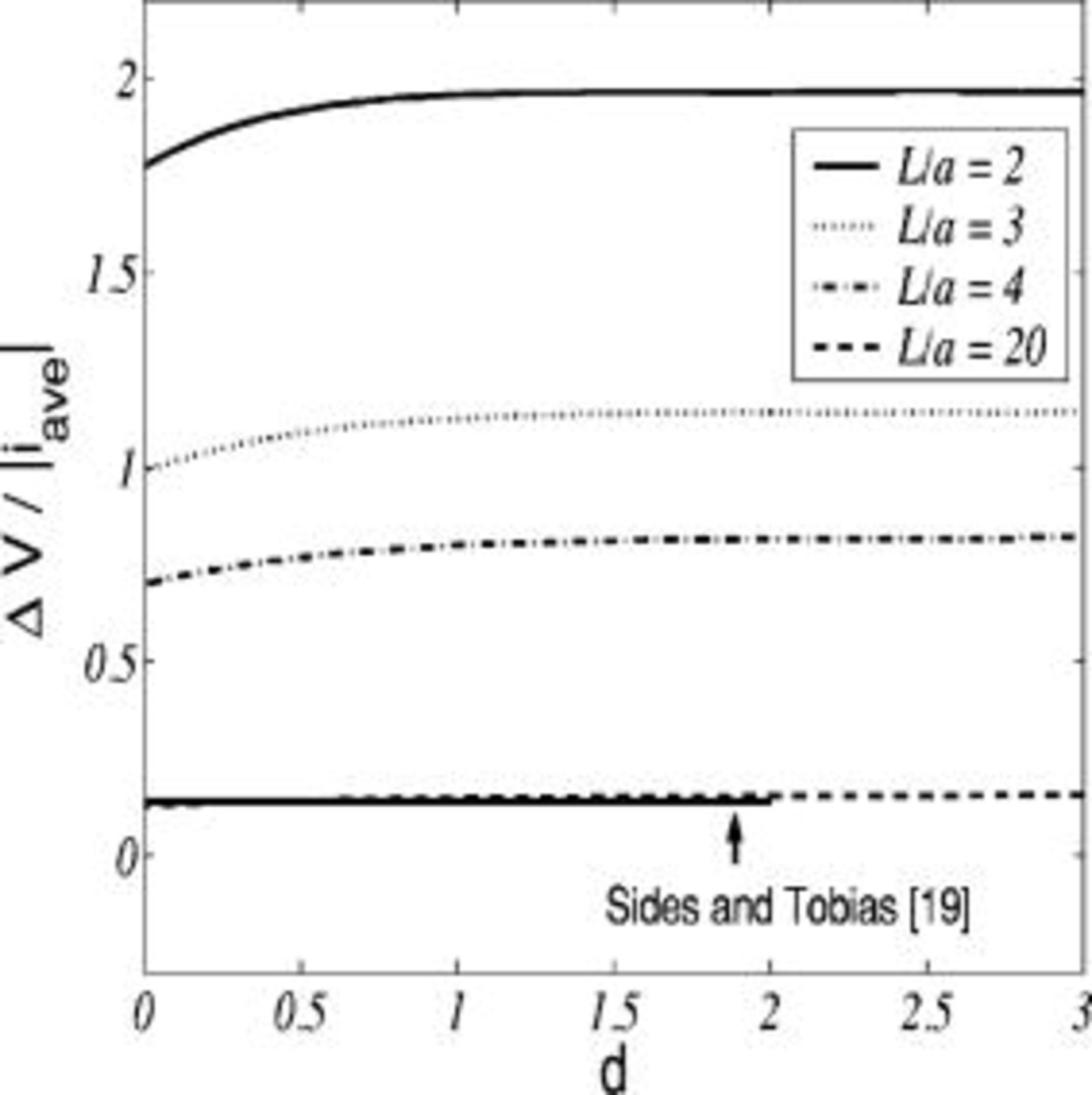
Figure 3. The resistance increment as a function of  , the minimum distance from the electrode to the particle, for various
 values.
The presence of an inert particle significantly affects the current density along a flat electrode as a particle moves in the vicinity of the electrode, which in turn affects the evolution of the growing metallic interface. When a particle is far enough away that there is no variation of potential field in the neighborhood of the electrode, the normalized current densities along the flat interface remain constant. As the distance between the particle and the electrode decreases, the normalized current density at the particle centerline  decreases to zero as the particle contacts the electrode. Obviously, current cannot pass through the nonconducting particle and goes around the particle. Figure 4 shows the variation of current density on the electrode with the particle’s vertical position, where the effect of the interparticle spacing is considered. The maximum value of the current density in the case of an attached particle
 is approximated to be at the two radius distances,19, 41 whereas the maximum value is at the boundary for other cases
 . Hence, we can expect the metallic deposited film away from the particle radius to grow faster than that near the particle.
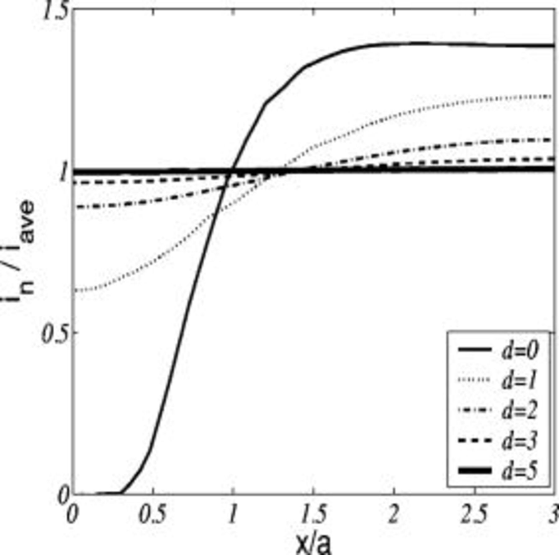
Figure 4. The primary current distribution along the flat electrode as a function of  for
 .
Figure 5a shows the evolution with time of a growing metallic film thickness for the particle entrapment process with a primary current distribution, where a flat interface is assumed as the initial condition. The moving speed of the metallic interface varies with the lateral coordinate, which depends on the normal derivative of potential field at the surface. The normalized current density with particle entrapment process is presented in Fig. 5b. The point of the maximum value of the normalized current density shifts from the edge of the boundary to near the particle radius, while within the distance  , the growing velocity reduces to zero in a way that the interface shape deforms largely around the particle and a void beneath the particle is formed, as illustrated in Fig. 5a.
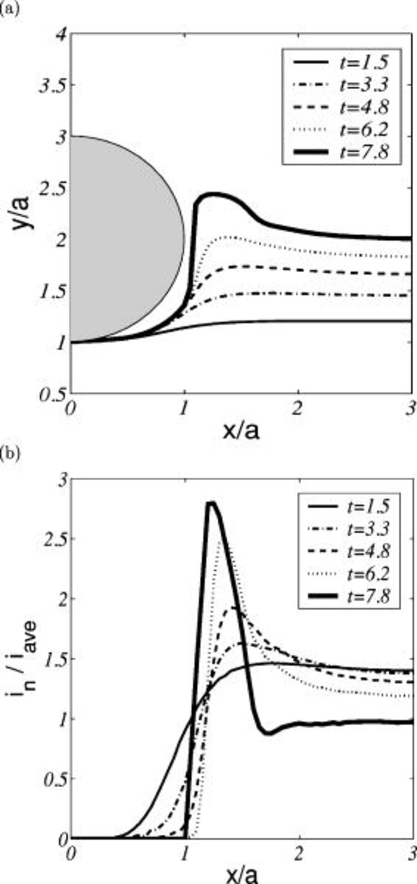
Figure 5. The primary current distribution with a growing metallic film ( and
 ): (a) temporal evolution of the metallic interface and (b) normalized current density.
The isocontour lines for electrical potential in Fig. 6a are parallel to each other in the regions far away from the particle, while the distribution of the potential near the particle is distorted in order to satisfy the insulating condition. The speed of the metallic interface then slows in the neighborhood of the particle compared with that away from the particle. As time goes on, the normal gradient of the electrical potential near the particle is so negligibly small that the surface appears stationary. However, the metallic surface away from the particle radius moves much faster, as shown in Fig. 6b. This is consistent with the analysis in Fig. 5b. As the surface grows at a distance equal to the particle radius in height, the interval of potential lines becomes smaller, so that the speed of the surface becomes larger, while the metallic interface near the particle does not grow. The metallic surface at  then grows faster and finally touches the particle. Figure 6b shows that voids near the particle are generated by the fast-developed moving metallic film that depends on the characteristics of the potential field. For the primary current distribution, the metallic film does not grow along the nonconducting particle surface.
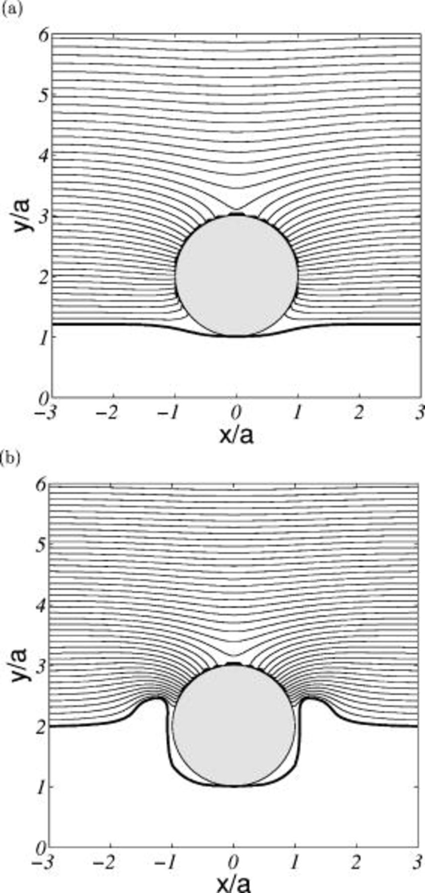
Figure 6. Potential distribution with a primary current distribution ( and
 ): (a)
 and (b)
 .
The level set function  corresponding to Fig. 6a and 6b is shown in Fig. 7a and 7b, where the curved thick line represents the zero level set of the metallic interface and the zero level set for a particle is overlapped as a circle. The zero level set of
 is initially a straight line, however it is deformed by following the speed function
 , the potential gradient in the normal direction defined by Eq. 16. Using the fast level set method, the level set function defined over the entire domain is extended by the values near the zero level set of
 . The incomplete and complete circular shapes inside the circle and the curved lines on top of the particle in Fig. 6a and 6b result from the extension of the curved shape of the zero level set of
 .
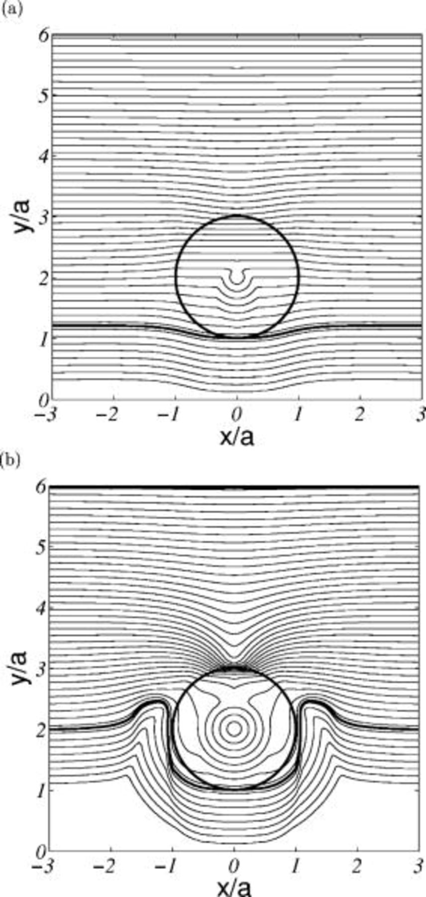
Figure 7. Level set function  at (a)
 and (b)
 , where the zero level set of
 is overlapped.
Secondary Current Distribution
In general, a more uniformly deposited film can be obtained with a secondary current density distribution.33 The difference from a primary current density distribution for the model is a nonlinear boundary condition at the electrode surface given by the Butler-Volmer equation which introduces a surface overpotential. Because the exchange current density  represents the kinetic speed of the reaction on the electrode,
 was used as a parameter in this study to investigate the effect of uniformity and growth of the deposited film.
In 1987, Dukovic and Tobias investigated the voltage increment of bubbles attached to a plane electrode as a function of current density and exchange current density.41 With a flat, fixed electrode, a secondary current density distribution in the presence of a particle was investigated to study the effect of the kinetics of the electrode reaction and to compare to results with a primary current density distribution. Figure 8a shows the normalized current density along the flat electrode for various values of  at small dimensionless exchange current density
 . When a particle comes into contact with an electrode,
 , the current density even at the contact point is a nonzero value. This makes for a more uniformly deposited film compared with that for a primary current density distribution. However, as
 increases to very large values (toward infinity), the pattern is similar to that of the primary current density distribution,41 as illustrated in Fig. 4. The resistance increment as a function of
 for a secondary current density distribution is compared to that for a primary current density distribution at the same condition in Fig. 8b. As
 increases, the resistance increment decreases and converges to a fixed value of that for a primary current density distribution. However, as the value of
 becomes smaller, the kinetic effects of the electrode reaction become important. This is a significant feature as compared with the primary current density distribution. The potential value underneath the particle decreases to compensate for the increased kinetic resistance, which will be discussed further in Fig. 11.
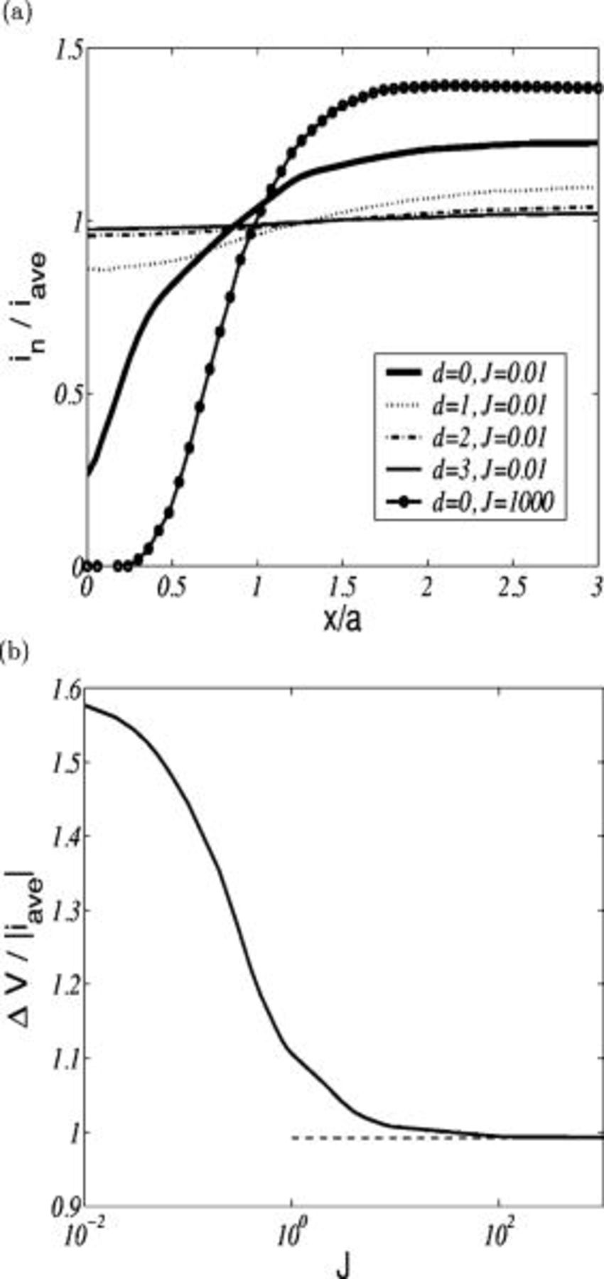
Figure 8. The secondary current distribution along a flat electrode  : (a) normalized current density as a function of normalized distance for various
 and
 values and (b) resistance increment as a function of
 , where a dashed line is for a primary current distribution.
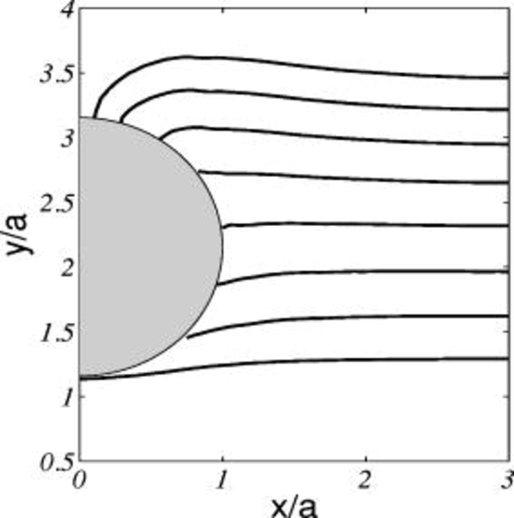
Figure 11. Temporal evolution with a secondary current distribution ( and
 ). The time step for each contour line is 0.5.
The evolution of the metallic interface with different  is illustrated in Fig. 9
 as the metallic interface is allowed to grow in proportion to current density along the interface. With a small exchange current density
 , as shown in Fig. 9a, the height difference along the surface is small as the deposited film grows with time. When a moderate exchange current density
 is considered, the growth of the metallic film below the particle in Fig. 9b is slower than that farther away from the particle. The corresponding current density along the surface is plotted in Fig. 10a. The current density at
 decreases as the film grows, while the current density at
 shows an almost constant value before the growing film touches the particle. This figure shows that the small void between the particle and the deposited film can be explained by both a geometrical effect and the potential characteristics. In the case of a large exchange current density
 , the difference in height with time, as shown in Fig. 9c, increases and a larger void beneath the particle compared to Fig. 9b is generated. The corresponding current density in Fig. 10b is very similar to that plotted in Fig. 5b. In order to show the void, the computation was stopped when the growing metallic film contacts the particle at
 for
 and for
 . The figures for the evolution of the growing deposited film and the current density distribution show that the primary current density distribution is the limiting case for the secondary current density distribution with a large exchange current density, as expected.
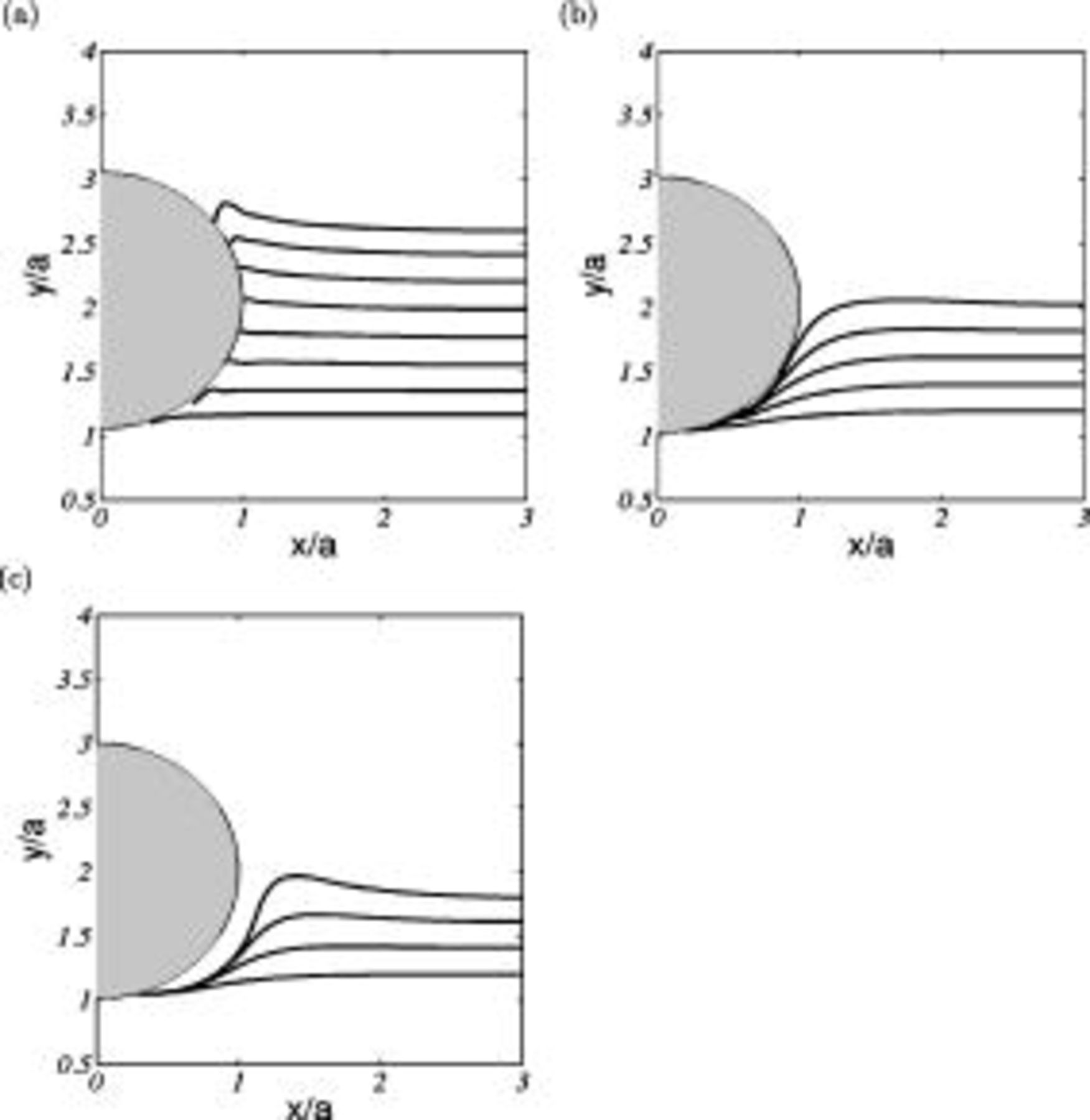
Figure 9. The temporal evolution of the metallic interface with a secondary current distribution  : (a)
 , (b)
 , and (c)
 . The regular time step for each contour line is 1.5.
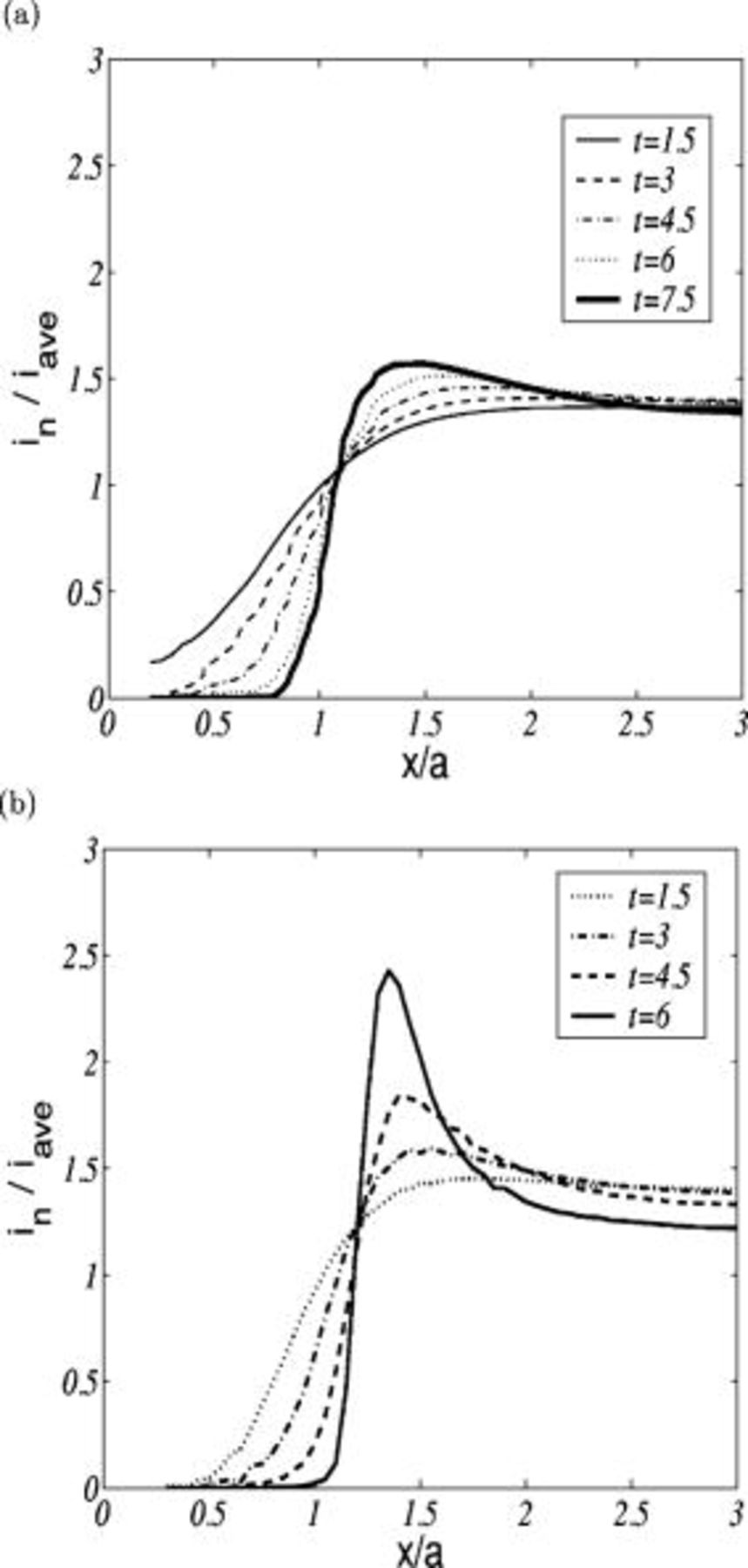
Figure 10. The secondary current distribution with a growing metallic film  : (a)
 and (b)
 .
Figure 11 shows the temporal evolution of a growing metallic film for the particle incorporation process with a large current density and a small exchange current density ( and
 ). As before, a flat interface is also considered initially. Unlike the primary current distribution in Fig. 5a, a good uniformity is shown, except on top of the particle. In order to explain the nonuniformity, the potential distributions were investigated in Fig. 12. When the particle contacts a growing metallic surface as shown in Fig. 12a, an interesting feature is that there exists distinct potential contour lines beneath the particle. These separated lines are induced by the kinetic resistance on the metallic interface and causes the current density near the particle to have a nonzero value. After the particle contacts the electrode surface, the growing film is uniform, as illustrated in Fig. 12c, where the potential lines are well distributed near the contact point between the particle and the metallic film, and the film’s growth, which is dependent upon potential gradient at the interface, is faster close to the particle. In Fig. 12e, the potential field at the gap between the developing film on both sides of the center line does not change much in the lateral direction; the normal gradient of potential on the metallic interface has nearly vanished. Therefore, the film grows vertically and does not extend into the gap such that a small void is generated on top of the particle. This indicates a possible mechanism for creation of a void even at a small exchange current density with a secondary current distribution. The level set functions
 corresponding to Fig. 12a, 12c and 12e are shown in Fig. 12b, 12d and 12f, respectively. The potential fields in Fig. 6a and 12a are different, while the level set function
 in Fig. 12b is similar to Fig. 7a, because the zero level set of
 at a contact time is similar for both cases. Because the metallic interface grows along the particle surface uniformly, the level set functions inside and outside the particle have a circular shape. The narrowly confined contour lines above the particle are induced by the highly curved zero level set in Fig. 12f.
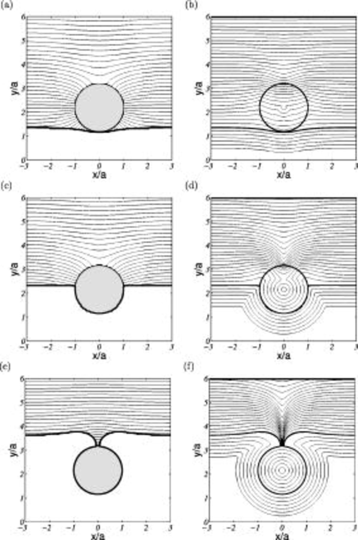
Figure 12. Secondary current distribution ( and
 ): (a), (c), and (e) potential distributions at
 ,
 , and
 and (b), (d), and (f) level set function
 corresponding to (a), (b) and (c), respectively, where the zero level set of
 is overlapped.
Conclusions
The primary and secondary current distributions with a growing metallic interface in the presence of a particle were investigated numerically. The potential field resolved by PLTMG was distorted by the nonconducting particle to satisfy the insulating boundary condition. The particle acted as an obstacle to a growing metallic film. In order to track this developing interface, the level set method was used.
For a primary current distribution, the resistance increment and the local current density distribution along the surface were affected by the presence of an insulating particle, and the influence was maximized when the particle contacted the electrode. The potential characteristics around the particle accelerated the growth speed of a deposited film near the particle radius, caused a large deformation of the metallic interface, and finally, created a void beneath the particle.
The kinetic resistance, which is dependent upon exchange current density, resulted in distinct potential lines underneath the particle with a secondary current distribution. The distinct potential field above the deposited film gave a nonzero current density along the surface and contributed to a more uniformly deposited film. However, a small void on top of the particle was generated even at a small exchange current density. The primary current density distribution was verified as the limiting case for the secondary current density distribution with large exchange current density through the resistance increment, the evolution of the growing metallic film, and the current density distribution along the surface.
This study showed a void generation mechanism with the primary and secondary current distributions induced by the presence of a nonconducting particle. The tertiary current distribution and the effect of a conducting particle in the particle incorporation process will be considered in future work. The lateral migration of the fluid will also be considered which will alter the concentration field, which in turn will cause the current density to change.
List of Symbols

| Hamaker constant, J |

| particle radius, m |

| concentration of ions, 
|

| minimum distance between a particle and an electrode normalized by 
|

| signed distance function, m |

| Faraday’s constant, 
|

| speed function for a level set method, m/s |

| deposited film thickness, m |

| minimum distance between a particle and an electrode, m |

| current density, 
|

| average current density 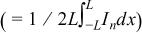 , 
|

| current density normal to the electrode, 
|

| exchange current density, 
|

| dimensionless current density |

| dimensionless average current density |

| dimensionless exchange current density 
|

| molar flux, 
|

| characteristic length scale in the  direction, m |

| molecular weight of the depositing species, kg/mol |

| unit normal vector pointing out an electrolyte solution |

| gas constant, J mol/K |

| absolute temperature, K |

| dimensionless time normalized by τ |

| time, s |

| velocity vector of a particle  , m/s |

| mobility of the particle, 
|

| potential at the cathode surface, V |

| growth rate normal to a deposited film, m/s |

| dimensionless growing speed normal to a deposited film |

| dimensionless potential difference between the top boundary and the metallic interface |

| position vector in Cartesian coordinate |

| interface position vector, m |

|
 component of center position of the particle, m |

|
 component of center position of the particle, m |

| initial position of a metallic interface in the  direction, m |

| charge number |

| charge number of the depositing species |
Greek

| anodic transfer coefficient |

| cathodic transfer coefficient |
| β | friction coefficient  , kg/s |

| surface overpotential, V |

| coefficients of the interpolated function 
|
| μ | viscosity of the electrolyte, Pa s |
| Φ | electrical potential, V |
| ϕ | dimensionless electrical potential |
| ψ | level set function, m |

| level set function for a particle |

| level set function for an initial metallic film |

| level set function for a growing metallic film |

| density of the cathodic deposit, 
|
| σ | electrical conductivity of the solution 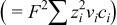 , S/m |
| τ | dimensionless time scale 
|
Acknowledgments
The authors greatly appreciate the discussion with Professor Bank concerning the use of the PLTMG program and Professor Cheng for the level set method in the Department of Mathematics at University of California, San Diego.
The University of California, San Diego assisted in meeting the publication costs of this article.
