


Abstract
The direction and magnitude of tundra vegetation productivity trends inferred from the normalized difference vegetation index (NDVI) have exhibited spatiotemporal heterogeneity over recent decades. This study examined the spatial and temporal drivers of Moderate Resolution Imaging Spectroradiometer Max NDVI (a proxy for peak growing season aboveground biomass) and time-integrated (TI)-NDVI (a proxy for total growing season productivity) on the Yamal Peninsula, Siberia, Russia between 2001 and 2018. A suite of remotely-sensed environmental drivers and machine learning methods were employed to analyze this region with varying climatological conditions, landscapes, and vegetation communities to provide insight into the heterogeneity observed across the Arctic. Summer warmth index, the timing of snowmelt, and physiognomic vegetation unit best explained the spatial distribution of Max and TI-NDVI on the Yamal Peninsula, with the highest mean Max and TI-NDVI occurring where summer temperatures were higher, snowmelt occurred earlier, and erect shrub and wetland vegetation communities were dominant. Max and TI-NDVI temporal trends were positive across the majority of the Peninsula (57.4% [5.0% significant] and 97.6% [13.9% significant], respectively) between 2001 and 2018. Max and TI-NDVI trends had variable relationships with environmental drivers and were primarily influenced by coastal-inland gradients in summer warmth and soil moisture. Both Max and TI-NDVI were negatively impacted by human modification, highlighting how human disturbances are becoming an increasingly important driver of Arctic vegetation dynamics. These findings provide insight into the potential future of Arctic regions experiencing warming, moisture regime shifts, and human modification, and demonstrate the usefulness of considering multiple NDVI metrics to disentangle the effects of individual drivers across heterogeneous landscapes. Further, the spatial heterogeneity in the direction and magnitude of interannual covariation between Max NDVI, TI-NDVI, and climatic drivers highlights the difficulty in generalizing the effects of individual drivers on Arctic vegetation productivity across large regions.
Export citation and abstract BibTeX RIS

Original content from this work may be used under the terms of the Creative Commons Attribution 4.0 license. Any further distribution of this work must maintain attribution to the author(s) and the title of the work, journal citation and DOI.
1. Introduction
Arctic vegetation plays a critical role in global climate feedbacks (Pearson et al 2013), permafrost dynamics (Blok et al 2010), and the distribution of herbivore populations connected to the livelihood of Arctic communities (Forbes and Kumpula 2009). Changes in Arctic vegetation since the 1980s have been monitored using the normalized difference vegetation index (NDVI) (Frost et al 2021), a proxy for primary productivity that remotely quantifies photosynthetically-active green vegetation (Reichle et al 2018). While NDVI and Arctic aboveground biomass have been found to have a weakly positive linear relationship (R2 = 0.23) at finer resolutions (<1 km) (Cunliffe et al 2020), there is evidence of a strong positive non-linear relationship (R2 = 0.94) between Arctic aboveground biomass and NDVI at coarser resolutions (⩾1 km), allowing in situ vegetation changes to be inferred from NDVI metrics at broader scales (Jia et al 2006, Epstein et al 2012, Raynolds et al 2012). Max NDVI (the greatest intra-annual NDVI value) represents peak growing season aboveground biomass, whereas time-integrated (TI)-NDVI (the sum of growing season NDVI values >0.05) represents total growing season productivity (Jia et al 2006, Bhatt et al 2021).
Despite net increases in Max NDVI and TI-NDVI since 1982 (Frost et al 2020), the direction and magnitude of Arctic vegetation productivity trends exhibit substantial spatiotemporal heterogeneity across multiple scales (e.g. local to continental, inter-annual to decadal) (Elmendorf et al 2012, Lara et al 2018, Berner et al 2020, Myers-Smith et al 2020). This spatiotemporal heterogeneity is likely due to complex vegetation interactions with climatic, geomorphic, biologic, and anthropogenic drivers (Walker et al 2009, Yu et al 2017, Frost et al 2021). While some of these relationships are well-studied, there are uncertainties in determining the relative importance of drivers across regions with varying climatological conditions, landscapes, and vegetation communities (Epstein et al 2004, Walker 2006, Dutrieux et al 2012, Bhatt et al 2021).
This study examined the effects of environmental and anthropogenic drivers on the spatial and temporal patterns of vegetation productivity on the Yamal Peninsula, Siberia, Russia (hereafter, the Peninsula) using NDVI metrics derived from Moderate Resolution Imaging Spectroradiometer (MODIS) data. The Peninsula is located in one of the warmer regions of the Arctic (Raynolds et al 2008), has steep climate and geomorphic gradients, ice-rich continuous permafrost, diverse Arctic vegetation, extensive indigenous reindeer herding, and burgeoning natural resource (gas) development (figure 1, Walker et al 2009). These conditions allowed it to serve as a case study for determining the critical drivers of Arctic vegetation productivity (Macias-Fauria et al 2012) under projected warming (IPCC 2021), increasing resource extraction (Walker 2010), and ongoing herbivory. Specifically, this study aimed to determine (1) which drivers exerted the greatest influence on the spatial distribution of Max and TI-NDVI across the Peninsula between 2001 and 2018, (2) the direction and magnitude of the Peninsula's Max and TI-NDVI trends between 2001 and 2018, and (3) which drivers best predicted variations in these trends.
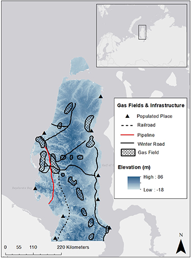
Figure 1. The Yamal Peninsula with elevation (m above sea level) and locations of population centers, infrastructure, and gas fields (Forbes 1999, Gazprom 2021). The inset map shows the location of the Yamal Peninsula.
Download figure:
Standard image High-resolution imageWe hypothesized that climatic drivers and physiognomic vegetation unit would best explain the spatial distribution of Max and TI-NDVI because of the influence of long-term climate patterns and growth form-specific physiological requirements on Arctic vegetation distribution (Walker et al 2002, Raynolds et al 2008). Additionally, we expected that Max and TI-NDVI trends would be positive across a majority of the Peninsula; however, spatial heterogeneity in trend magnitude and direction was expected due to variable climatological and landscape conditions. Lastly, we hypothesized that geomorphic and anthropogenic drivers would best explain variations in Max and TI-NDVI trends due to their ability to mediate the effects of climate on vegetation productivity.
2. Methods
2.1. Study area
The Peninsula is located within the Arctic tundra of northwestern Siberia, Russia and is approximately 600 km long (south–north, including Belyy Island in the north) and up to 250 km wide (Walker et al 2009). Between 2001 and 2018, the mean annual temperature ranged from −13 °C to −8 °C (Wan et al 2015), and mean annual precipitation ranged from 240 to 367 mm (Abatzoglou et al 2018). The Peninsula has predominantly flat topography (figure 1), with a majority of slopes < 7°, and elevations reaching 86 m above sea level (Leibman et al 2014, Rizzoli et al 2017). The landscape is underlain by ice-rich continuous permafrost and dominated by river networks, sandy ridges, and lowland valleys with abundant thermokarst lakes, drained thermokarst lake basins, and polygonal peatlands (Walker et al 2009, Verdonen et al 2020). Cryogenic landslides controlled by active layer depth and soil water content are the primary disturbance process on the Peninsula (Leibman 1995, Macias-Fauria et al 2012, Leibman et al 2014). Vegetation transitions from erect low shrub tundra in the south to sedge, prostrate dwarf-shrub, and moss tundra in the north (supplementary figure 1, Walker et al 2009). Shrubs are present throughout the Peninsula, but increase in abundance from north to south (Epstein et al 2021).
2.2. Data sources and pre-processing
This study employed Max and TI-NDVI derived from the MODIS Vegetation Indices product and a suite of climatic, geomorphic, biologic, and anthropogenic drivers (table 1). A lack of quantitative data and exclusion areas limited the potential for a meaningful assessment of reindeer effects as a biologic driver (Walker et al 2009).
Table 1. Datasets included in the analyses. *Dependent variables.
| Data type | Year(s) included | Dataset(s) | Definition | Native resolution | Source |
|---|---|---|---|---|---|
| Continuous | N/A | Distance from the Coast | Kilometers from the coast; considered a proxy for sea ice influence on temperature and precipitation | 1 km | Circumpolar Arctic Vegetation Map (Walker and Raynolds 2018) |
| N/A | Elevation | N/A | 90 m | TanDEM-X 90 m Digital Elevation Model (Rizzoli et al 2017) | |
| 2001–2018 | Human modification | Cumulative measure of the area impacted by natural resource extraction, infrastructure, and settlements | 1 km | Conservation Science Partners (Kennedy et al 2019) | |
| 2001–2018 | Max NDVI* | Annual peak NDVI value | 250 m | Terra MODIS Vegetation Indices (MOD13Q1.006) (Didan 2015) | |
| 2001–2018 | Precipitation and soil moisture | Mean snow-free season (April–September) precipitation and soil moisture | 2.5 arc minutes | TerraClimate: Monthly Climate and Climatic Water Balance for Global Terrestrial Surfaces, University of Idaho (Abatzoglou et al 2018) | |
| 2001–2018 | Snow-free period onset | First day of the year with 0% snow cover | 500 m | Terra MODIS Snow Cover (MOD10A1.006) (Hall et al 2016, Armstrong et al 2022) | |
| 2001–2018 | Summer warmth index | Sum of April–September monthly mean temperatures >0 °C | 1 km | Terra MODIS Land Surface Temperature and Emissivity (MOD11A1.006) (Wan et al 2015) | |
| 2001–2018 | TI-NDVI* | Annual sum of NDVI values >0.05 | 250 m | Terra MODIS Vegetation Indices (MOD13Q1.006) (Didan 2015) | |
| Categorical | N/A | Landscape age | Time since last glaciation | 1 km | Circumpolar Arctic Vegetation Map (Walker and Raynolds 2018) |
| N/A | Physiognomic vegetation unit | N/A | 1 km | Circumpolar Arctic Vegetation Map (Walker and Raynolds 2018) | |
| N/A | Soil texture | N/A | 1 km | Circumpolar Arctic Vegetation Map (Walker and Raynolds 2018) | |
| N/A | Substrate chemistry | N/A | 1 km | Circumpolar Arctic Vegetation Map (Walker and Raynolds 2018) |
Pre-processing was completed using Google Earth Engine (GEE), ArcGIS (Redlands, CA), and R version 4.0.0 (R Core Team 2020). Pre-processing entailed evaluating pixel quality, masking surface water, deriving the parameter of interest for the 2001–2018 study period, and resampling to a 1 km spatial resolution to ensure that the datasets were comparable. Low-quality pixels affected by cloud cover, aerosols, and viewing angle are removed from the operational data products used in this study (FAO/IIASA/ISRIC/ISS-CAS/JRC 2012, Didan 2015, Wan et al 2015, Hall et al 2016, Rizzoli et al 2017, Abatzoglou et al 2018, Walker and Raynolds 2018, Kennedy et al 2019). Marginal-quality pixels were used to supplement the spatial coverage of snow-free period onset, summer warmth index (SWI), Max NDVI, and TI-NDVI datasets when high-quality data were unavailable. Permanent surface water bodies were masked using the GlobCover Global Land Cover Map (ESA and UC Louvain 2010). A 1 km resolution was used for the analyses because it was the native resolution of the majority of the datasets considered (7 of the 12), which minimized the number of datasets that needed to be resampled (table 1).
2.3. Max and TI-NDVI calculation
The MODIS Vegetation Indices product (MOD13Q1.006) provides NDVI calculated using the equation (NIR − R)/(NIR + R), where NIR equals the reflectance of near-infrared radiation and R equals the reflectance of visible red radiation (Didan 2015). This MODIS product was used because it is comprised of NDVI values derived from 16 day maximum value composite images (hereafter, composites), which allowed for better temporal data quality screening than other available products. The annual Max NDVI for each pixel was determined by selecting the maximum NDVI value from composites covering 26 June–13 September (period of peak vegetation productivity on the Peninsula). Barren, snow-covered, and ephemeral water-covered land surfaces were excluded by masking pixels with Max NDVI values below 0.1 (Raynolds et al 2006). Annual TI-NDVI for each pixel was calculated by summing NDVI values above 0.05 from composites covering the entire snow-free season (April–September) (Bhatt et al 2021). Each time-period composite included in the Max and TI-NDVI calculations had variable spatial coverage due to the exclusion of low-quality pixels affected by water, clouds, heavy aerosols, and cloud shadows (Didan 2015). Therefore, the number of pixels masked varied for each composite but did not exceed 4.5% for Max NDVI or 12.5% for TI-NDVI. At the pixel scale, this resulted in variable intra-annual coverage and a bias toward artificially low Max and TI-NDVI values. This bias was removed by only calculating annual Max and TI-NDVI for a pixel when data from all time-period composites considered were available. Max and TI-NDVI calculations were completed using GEE.
2.4. Spatial correlations among Max NDVI, TI-NDVI, and continuous drivers
Pairwise Spearman's correlation was used to determine the direction and significance of the spatial relationships among Max NDVI, TI-NDVI, and the continuous drivers (table 1). The 2001–2018 means of Max NDVI, TI-NDVI, and climatic drivers were included as inputs, and all other included variables (coast distance, elevation, and human modification) were constant over the 2001–2018 study period. Although human modification is dynamic, the dataset used here provides a cumulative measure of human modification based on the spatial extent of settlements, agriculture, transportation, mining, energy production, and electrical infrastructure in 2016 (Kennedy et al 2019). The Bonferroni correction was applied to account for multiple comparisons. Spearman's correlations were also run on stratified random samples using 2/3 and 1/2 of the input dataset to determine if the results were impacted by spatial autocorrelation. Spearman's correlation was implemented using the psych package in R (R Core Team 2020, Revelle 2020).
2.5. Spatial correlations among Max NDVI, TI-NDVI, and categorical drivers
Chi-square (χ2) tests of independence were employed to determine if there were significant spatial associations among 2001–2018 mean Max-NDVI, TI-NDVI and categorical drivers (table 1). Mean Max and TI-NDVI were divided into high, mid-, and low categories using the Jenk's natural breaks classification method (implemented using the BAMMtools package in R) (Rabosky et al 2014, R Core Team 2020). Chi-square tests of Independence were also run on stratified random samples using 2/3 and 1/2 of the input datasets to determine if the results were impacted by spatial autocorrelation. The χ2 test statistics and residuals were compared to determine the direction and significance of the spatial associations.
2.6. Trend detection
Mann-Kendall trend tests were implemented to detect the presence of pixel-scale monotonic trends in Max NDVI, TI-NDVI, and climatic drivers between 2001 and 2018. Pixels with fewer than 15 years of data due to the masking of low-quality pixels (described further in section 2.3) were excluded from the analyses (3.9% of the Max NDVI dataset and 4.7% of the TI-NDVI dataset). The Durbin–Watson test found that <5% of pixels exhibited significant lag-1 serial autocorrelation (Kulkarni and von Storch 1995). Modified Mann–Kendall trend tests were run to verify that pixels with significant serial autocorrelation did not affect trend significance. Sen's slope estimation was used to determine the direction and magnitude of Max NDVI, TI-NDVI, and climatic driver trends. Trend detection analyses were completed using the car (Fox and Weisberg 2019), Kendall (McLeod 2011), modifiedmk (Patakamuri and O'Brien 2020), and trend packages (Pohlert 2020) in R. GEE was used to calculate 2001–2009 and 2010–2018 mean NDVI values for each time-period composite included in the analysis to illustrate shifts in Max NDVI and TI-NDVI between the first and second halves of the study period.
2.7. Drivers of Max and TI-NDVI trends
Random forest regression (RFR) models were used to determine the best predictors of Max and TI-NDVI trends (Sen's slopes) across the Peninsula. All drivers were included as explanatory variables in the models, and the Sen's slopes of climatic drivers were used (table 1). A pairwise Spearman's correlation was used to confirm that multicollinearity (r > 0.75 or <−0.75) was not present among the continuous input drivers (Berner et al 2020). RFR models were trained using bootstrapped data and tuned to determine the number of randomized drivers considered at each tree node (mtry = 5) that resulted in the lowest mean square error (MSE) (Oliveira et al 2012). The mean decrease in accuracy (% IncMSE) metric was used to determine variable importance (Liaw and Wiener 2002). Additional RFR models were run for areas where significant Max and TI-NDVI trends were observed to determine if the best predictors of trends across the Peninsula were also driving change in these areas. RFR modeling was completed using the caret (Kuhn 2020), randomForest (Liaw and Wiener 2002), and doParallel packages (Microsoft and Weston 2020) in R.
The relationships between Max/TI-NDVI trends and the six most important drivers identified by the RFR models were evaluated using partial dependence plots. Pixel-scale Spearman's correlations were run between linearly-detrended Max/TI-NDVI and the three most important climatic driver time series (precipitation, soil moisture, and SWI) to assess their interannual covariation irrespective of trends, and therefore what drove variability in Max and TI-NDVI year to year. Linear detrending was completed by modeling a linear function and then subtracting the function from the observed data. These analyses were completed using the pdp (Greenwell 2017), pracma (Borchers 2019), and psych packages (Revelle 2020) in R.
3. Results
3.1. Continuous spatial drivers of Max and TI-NDVI
Correlations between time-averaged parameters over the 2001–2018 study period were evaluated to determine the strength of their spatial relationships. There was a significant (p-value < 0.05), strong, and positive spatial correlation between mean Max and TI-NDVI (r = 0.93, figure 2 and supplemental figure 2). Mean Max NDVI exhibited the strongest significant spatial correlations with mean SWI (r = 0.40), mean precipitation (r = 0.39), and mean snow-free period onset date (r = −0.40), as well as weaker but significant correlations with the other continuous drivers (except for elevation). Mean Max NDVI was positively correlated with human modification (r = 0.27) and weakly correlated with mean soil moisture (r = 0.02) and coast distance (r = −0.02). Therefore, areas with higher Max NDVI coincided with higher SWI, higher precipitation, earlier snowmelt, and higher human modification, whereas Max NDVI exhibited little to no spatial relationship with soil moisture, coast distance, or elevation. Mean TI-NDVI exhibited similar spatial relationships with the continuous drivers; however, mean TI-NDVI was not significantly correlated with mean soil moisture, and was better correlated with mean SWI, mean precipitation, mean snow-free period onset date, human modification, coast distance, and elevation than mean Max NDVI (figure 2). Results were similar for analyses run on stratified random samples using 2/3 and 1/2 of the input dataset.

Figure 2. Spearman's correlation coefficients (r) for correlations between Max NDVI, TI-NDVI, and continuous drivers. The 2001–2018 means of Max NDVI, TI-NDVI, precipitation (Precip), snow-free period onset date (SnowFree), soil moisture, and summer warmth index (SWI) were used. Human modification (HumanMod), elevation, and coast distance (CoastDist) values included were constant over the study period. Max and TI-NDVI correlations are highlighted by the thicker black boxes. *Insignificant at the 95% confidence level.
Download figure:
Standard image High-resolution imageNotable spatial correlations among the continuous drivers were present. Mean precipitation was positively correlated with mean SWI (r = 0.89), and both mean precipitation and mean SWI were negatively correlated with mean snow-free period onset date (r = −0.86 and −0.85, respectively; figure 2 and supplemental figure 3). Human modification was positively correlated with mean SWI (r = 0.32) and mean precipitation (r = 0.47), and negatively correlated with mean snow-free period onset date (r = −0.44); therefore, on average, human settlement more frequently coincided with higher SWI, higher precipitation, earlier snowmelt. Additionally, coast distance was positively correlated with elevation (r = 0.63) and mean SWI (r = 0.40), and negatively correlated with mean soil moisture (r = −0.72), indicating that mean elevation and SWI increased with distance from the coast while soil moisture decreased.
3.2. Categorical spatial drivers of Max and TI-NDVI
Vegetation unit had the strongest spatial association with mean Max NDVI categories ( 2 = 10 674), followed by substrate chemistry (
 2 = 5672), soil texture (
 2 = 2337), and landscape age (
 2 = 128). Similarly, vegetation unit had the strongest spatial association with mean TI-NDVI categories (
 2 = 25 903), followed by soil texture (
 2 = 3747), substrate chemistry (
 2 = 2966), and landscape age (
 2 = 1748). High mean Max and TI-NDVI were associated with erect shrub and wetland vegetation (a combination of sedges, mosses, and erect shrubs) (Raynolds et al
2006), whereas low mean Max and TI-NDVI were associated with graminoid and prostrate shrub vegetation. High mean Max and TI-NDVI were associated with circumneutral substrates, whereas low mean Max and TI-NDVI were associated with acidic and saline substrates. Last, high mean Max and TI-NDVI were associated with fine-textured soils, whereas low mean Max and TI-NDVI were associated with coarse-textured soils. Mean Max and TI-NDVI exhibited slightly different relationships with landscape age. High mean Max NDVI was associated with older landscapes (∼70 000 years old), and low mean Max NDVI was associated with younger (∼25 000 years old) and recently disturbed landscapes (∼1000 years old). Mid-mean TI-NDVI was associated with older landscapes (result not shown), whereas high and low mean TI-NDVI were associated with younger landscapes. Low mean TI-NDVI was also associated with recently disturbed landscapes. Results were similar for analyses run on stratified random samples using 2/3 and 1/2 of the input datasets (table 2).
2 = 1748). High mean Max and TI-NDVI were associated with erect shrub and wetland vegetation (a combination of sedges, mosses, and erect shrubs) (Raynolds et al
2006), whereas low mean Max and TI-NDVI were associated with graminoid and prostrate shrub vegetation. High mean Max and TI-NDVI were associated with circumneutral substrates, whereas low mean Max and TI-NDVI were associated with acidic and saline substrates. Last, high mean Max and TI-NDVI were associated with fine-textured soils, whereas low mean Max and TI-NDVI were associated with coarse-textured soils. Mean Max and TI-NDVI exhibited slightly different relationships with landscape age. High mean Max NDVI was associated with older landscapes (∼70 000 years old), and low mean Max NDVI was associated with younger (∼25 000 years old) and recently disturbed landscapes (∼1000 years old). Mid-mean TI-NDVI was associated with older landscapes (result not shown), whereas high and low mean TI-NDVI were associated with younger landscapes. Low mean TI-NDVI was also associated with recently disturbed landscapes. Results were similar for analyses run on stratified random samples using 2/3 and 1/2 of the input datasets (table 2).
Table 2. Chi-square test of independence results. All tests were significant at the 95% confidence level. Bolded residual values with the largest absolute values had the greatest influence on the spatial associations. Positive residuals indicate a positive relationship and negative residuals indicate a negative relationship. The mid-mean Max and TI-NDVI categories are excluded because the most influential relationships were associated with high and low mean Max and TI-NDVI categories.
| Drivers | Chi-square test of independence residuals | ||||
|---|---|---|---|---|---|
| Mean Max NDVI | Mean TI-NDVI | ||||
| High | Low | High | Low | ||
| Vegetation unit | Erect shrub | 41.0 | −43.8 | 72.3 | −66.1 |
| Graminoid | −30.3 | 33.5 | −66.8 | 48.2 | |
| Prostrate shrub | −43.5 | 49.5 | −57.4 | 65.1 | |
| Wetland | 9.5 | −15.9 | 22.5 | −8.6 | |
| Substrate chemistry | Acidic | −22.4 | 15.8 | −2.4 | 17.7 |
| Circumneutral | 50.7 | −36.5 | 6.1 | −41.3 | |
| Saline | −0.9 | 5.3 | −4.7 | 10.9 | |
| Soil texture | Clay loam | 7.2 | −10.1 | 7.7 | −6.3 |
| Loam | −2.3 | 5.1 | −11.2 | 5.2 | |
| Sand | −4.4 | 8.0 | −9.7 | 12.4 | |
| Sandy loam | −28.1 | 16.5 | −30.7 | 20.6 | |
| Silt loam | 18.8 | −14.8 | 32.0 | −18.5 | |
| Landscape age | Older | 3.9 | −5.6 | −2.4 | −28.5 |
| Younger | −1.7 | 2.1 | 1.1 | 12.2 | |
| Recently disturbed | −0.9 | 7.3 | −0.4 | 8.9 | |
Note: Bold indicates the most influence on the spatial associations.
3.3. Max and TI-NDVI trends
Max and TI-NDVI increased across a majority of the Peninsula between 2001 and 2018 (figure 3). Max NDVI trends were positive across 57.4% of the Peninsula (5.0% significant positive trends [p-value < 0.05]) and negative across 17.8% (0.6% significant negative trends). Additionally, 25.4% of the Peninsula exhibited no Max NDVI trend (p-value > 0.05 and Sen's slope = 0.000). Max NDVI Sen's slope ranged from −0.022 to 0.045 yr−1, with the mode between 0.000 and 0.001 yr−1. TI-NDVI trends were positive across 97.6% of the Peninsula (13.9% significant positive trends) and negative across 1.9% (<0.1% significant negative trends). Only 0.4% of the Peninsula exhibited no TI-NDVI trend. TI-NDVI Sen's slope ranged from −0.130 to 0.238 yr−1, with the mode between 0.020 and 0.030 yr−1. Overall, 71.5% of the Peninsula exhibited simultaneous increases in Max and TI-NDVI, 1.4% exhibited simultaneous decreases, and 27.1% exhibited divergent trends (figure 4). The direction and magnitude of climatic driver trends were variable (supplemental figure 4).
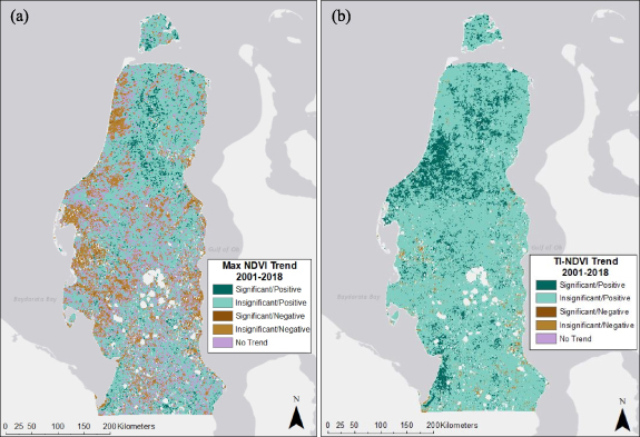
Figure 3. Trends in (a) Max NDVI and (b) TI-NDVI inferred from Mann–Kendall trend tests and Sen's slope estimation. Pixels were classified based on trend significance at the 95% confidence level and Sen's slope direction. Pixels classified as no trend had insignificant trends and Sen's slopes = 0.000. Permanent water bodies and pixels with < 15 years of data (due to low quality data or conditions preventing vegetation growth) were masked.
Download figure:
Standard image High-resolution image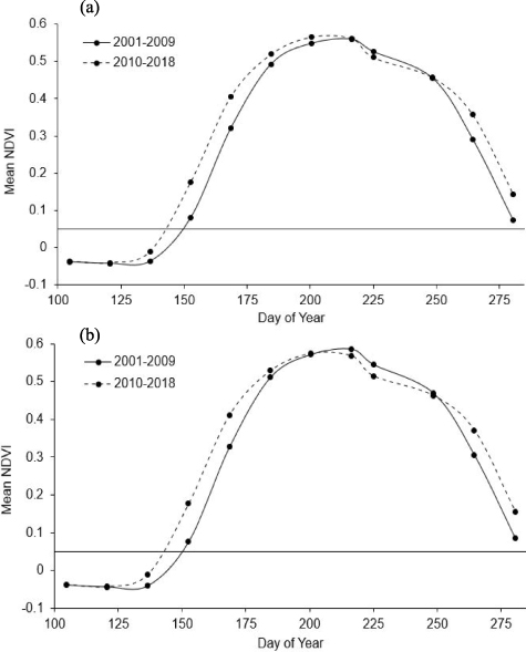
Figure 4. Phenology curves for pixels where (a) Max and TI-NDVI increased and (b) where Max NDVI decreased while TI-NDVI increased. Mean 2001–2009 and 2010–2018 NDVI values were calculated for each 16-day growing season composite image to assess how Max and TI-NDVI shifted between the first and second halves of the study period. Max NDVI is represented by the peak mean NDVI value at the top of each curve, and TI-NDVI is represented by the area under the curve. The line at mean NDVI = 0.05 indicates the minimum threshold for NDVI values included in TI-NDVI calculation.
Download figure:
Standard image High-resolution image3.4. Drivers of Max and TI-NDVI trends
The Max NDVI RFR model for the entire Peninsula explained 65% of Max NDVI Sen's slope variance, and the model for areas with significant Max NDVI trends explained 76%. The most important drivers of Max NDVI trends across the Peninsula were coast distance, human modification, soil moisture Sen's slope, precipitation Sen's slope, elevation, and SWI Sen's slope (supplemental figure 5). These were also the most important drivers of significant Max NDVI trends; however, precipitation and SWI trends were better predictors in these areas (supplemental figure 6). Driver relationships with Max NDVI trends were similar across the entire Peninsula and areas that exhibited significant change (supplemental figure 7). Due to the limited spatial extent of significant trends, the results discussion focuses on findings for the entire Peninsula.
On average, positive Max NDVI trends were strongest further inland, at higher elevations, and where SWI trends exceeded approximately 0.5 °C months yr−1 (figure 5). However, some strong, positive Max NDVI trends occurred along the southeastern coastline at elevations between −15 m and −13 m (below sea level) (<1.0% of pixels). Additionally, only 1.7% of the Peninsula experienced increases in SWI greater than 0.5 °C months yr−1 (equivalent to a cumulative SWI increase of greater than 9 °C months). Prior to reaching this threshold, Max NDVI and SWI trends exhibited a slightly negative relationship. The covariation between detrended Max NDVI and SWI time series was variable, with 53.9% of pixels exhibiting a negative correlation (4.9% significant, p-value < 0.05) and 46.1% exhibiting a positive correlation (3.5% significant) (figure 6).

Figure 5. Partial dependence plots for the six most important drivers of Max NDVI Sen's slope across the Peninsula (significant and insignificant trends): distance from the coast, human modification, mean growing season soil moisture Sen's slope, mean growing season precipitation Sen's slope, elevation, and summer warmth index (SWI) Sen's slope. Partial dependence plots display the average predicted relationships between Max NDVI trends and individual drivers across their range of values while still considering the average effects of the other drivers (Goldstein et al 2015). Dashed lines indicate outlier driver variable values.
Download figure:
Standard image High-resolution image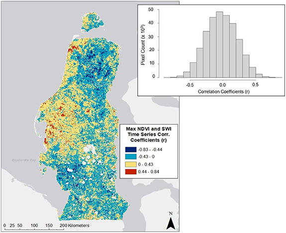
Figure 6. Map of Spearman's correlation coefficients (r) for pixel-wise correlations between linearly detrended Max NDVI and SWI time series (2001–2018). The inset histogram displays the frequency of r values across the Yamal Peninsula.
Download figure:
Standard image High-resolution imagePositive Max NDVI trends were also strongest where human modification was limited and where soil moisture and precipitation trends were negative (figure 5). Most pixels had less than 3% of their area modified by human activities; however, pixels with 30% or more modified area exhibited negative Max NDVI trends. Detrended Max NDVI and soil moisture time series were negatively correlated across 68.5% of the Peninsula (4.5% significant) and positively correlated across 31.5% (1.5% significant) (figure 7). Similarly, detrended Max NDVI and precipitation time series were negatively correlated across 62.8% of the Peninsula (4.3% significant) and positively correlated across 37.2% (1.6% significant) (supplemental figure 8). These correlations, although spatially variable, indicate that above-average Max NDVI co-occurred with below-average soil moisture and precipitation across a majority of the Peninsula.
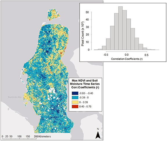
Figure 7. Map of Spearman's correlation coefficients (r) for pixel-wise correlations between linearly detrended Max NDVI and mean growing season soil moisture time series (2001–2018). The inset histogram displays the frequency of r values across the Yamal Peninsula.
Download figure:
Standard image High-resolution imageThe TI-NDVI RFR model for the entire Peninsula explained 70% of TI-NDVI Sen's slope variance, and the model for areas with significant TI-NDVI trends explained 73%. Max and TI-NDVI Sen's slopes (across the Peninsula and where trends were significant) were best predicted by the same six variables; however, the importance of these variables varied (supplemental figures 5 and 6). The most important drivers of TI-NDVI trends across the Peninsula were coast distance, elevation, precipitation Sen's slope, human modification, SWI Sen's slope, and soil moisture Sen's slope. Human modification and SWI Sen's slope were more important where TI-NDVI trends were significant (supplemental figure 6). Driver relationships with TI-NDVI trends were similar across the entire Peninsula and areas that exhibited significant change, with the exception of soil moisture trends and elevation (supplemental figure 9). Similarly to Max NDVI trends, the results discussion focuses on findings for the entire Peninsula.
On average, positive TI-NDVI trends were strongest at higher elevations, where SWI trends exceeded approximately 0.1 °C months yr−1, and where soil moisture trends were slightly positive around 0.5 mm yr−1 (figure 8). The positive relationship between TI-NDVI and SWI trends became stronger after SWI Sen's slopes reached 0.5 °C months yr−1. Detrended TI-NDVI and SWI time series were positively correlated across 99.9% of the Peninsula (78.1% significant), indicating that annual TI-NDVI and SWI positively covaried across nearly the entire Peninsula (figure 9). Positive TI-NDVI trends were consistently stronger where soil moisture Sen's slopes were less negative and approaching 0 mm yr−1. Detrended TI-NDVI and soil moisture time series were negatively correlated across 67.1% of the Peninsula (6.8% significant) and positively correlated across 32.8% (0.7% significant) (figure 10). Therefore, although TI-NDVI and soil moisture trends exhibited a positive relationship, they did not positively covary interannually across a majority of the Peninsula.
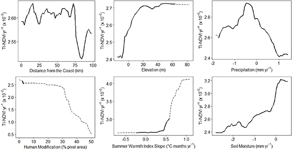
Figure 8. Partial dependence plots for the six most important drivers of TI-NDVI Sen's slope across the Peninsula (significant and insignificant trends): distance from the coast, elevation, mean growing season precipitation Sen's slope, human modification, summer warmth index (SWI) Sen's slope, and mean growing season soil moisture Sen's slope. Partial dependence plots display the average predicted relationships between TI-NDVI trends and individual drivers across their range of values while still considering the average effects of the other drivers (Goldstein et al 2015). Dashed lines indicate outlier driver variable values.
Download figure:
Standard image High-resolution image
Figure 9. Map of Spearman's correlation coefficients (r) for pixel-wise correlations between linearly detrended TI-NDVI and SWI time series (2001–2018). The inset histogram displays the frequency of r values across the Yamal Peninsula.
Download figure:
Standard image High-resolution image
Figure 10. Map of Spearman's correlation coefficients (r) for pixel-wise correlations between linearly detrended TI-NDVI and mean growing season soil moisture time series (2001–2018). The inset histogram displays the frequency of r values across the Yamal Peninsula.
Download figure:
Standard image High-resolution image
Positive TI-NDVI trends were also strongest closer to the coast, where precipitation trends were negative, and where human modification was limited (figure 8). TI-NDVI trends fluctuated with distance from the coast but were strongest between 0 and 75 km inland. The relationship between TI-NDVI and precipitation trends was unimodal, with the strongest TI-NDVI trends occurring where precipitation decreased by approximately 0.5 mm yr−1. Detrended TI-NDVI and precipitation time series were positively correlated across 76.6% of the Peninsula (1.5% significant) and negatively correlated across 26.3% (<0.1% significant); therefore, TI-NDVI and precipitation positively covaried interannually across a majority of the Peninsula, despite the trends exhibiting a negative relationship where precipitation trends were greater than −0.5 mm yr−1 (supplemental figure 10). As with Max NDVI trends, positive TI-NDVI trends were weakest where 30% or more of the area had been modified by humans.
4. Discussion
4.1. Spatial drivers of Max NDVI and TI-NDVI
Climatic drivers and physiognomic vegetation unit best explained the spatial distribution of Max NDVI and TI-NDVI on the Peninsula. On average, areas with higher Max and TI-NDVI coincided with warmer summer temperatures, higher precipitation, earlier snow melt, and vegetation units dominated by erect shrubs and wetland vegetation. Although soil moisture has been found to influence Arctic vegetation distribution (Walker et al 2001, Raynolds et al 2008, van der Kolk et al 2016) and has a more direct effect on water availability than precipitation, it did not exhibit a spatial correlation with Max or TI-NDVI. This implies that the positive spatial correlations among Max/TI-NDVI and precipitation may have been driven by the strong spatial relationships that precipitation has with SWI and snow-free period onset date, rather than spatial patterns of water availability.
In addition to influencing water availability (Gamon et al 2013), the timing of snowmelt determines when the growing season can begin (Bieniek et al 2015). Vegetation distribution may have been more limited by summer warmth and growing season onset than water availability because of the continuous permafrost underlying the Peninsula and the mostly shallow active layer depths (Leibman et al 2015) that restrict drainage and generally facilitate high soil moisture conditions (Bieniek et al 2015). Additionally, our results are consistent with findings that more productive Arctic vegetation with higher aboveground biomass is found where growth is not limited by low temperatures or shorter growing seasons (Jia et al 2006, Raynolds et al 2006, Epstein et al 2021).
The positive spatial correlations between Max/TI-NDVI and human modification were likely the result of warmer, coastal areas with earlier snowmelt also coinciding with more human activity. However, re-vegetated off-road vehicle tracks on the Peninsula near concentrated areas of infrastructure have been found to have higher aboveground biomass than surrounding undisturbed areas approximately 20 years after revegetation (Forbes et al 2009). Ground verification and/or comparison with finer resolution imagery would be needed to confirm if this occurred in other re-vegetated areas that were previously impacted by human activities.
Although less important than vegetation unit, substrate chemistry, soil texture, and landscape age also influenced spatial patterns of Max NDVI and TI-NDVI. Max and TI-NDVI were highest on nutrient-rich circumneutral substrates and fine-textured soils, similar to other studies from the region (Walker et al 2005, Macias-Fauria et al 2012, Epstein et al 2021). The weak positive association between high TI-NDVI and younger landscapes was unexpected because older landscapes can have greater nutrient availability and erect shrub coverage after the development of fine-grained soils and stream networks, vegetation succession, and peat accumulation (Walker et al 1995). However, the negative spatial association between high TI-NDVI and younger landscapes was stronger and drove the significance of the spatial relationship between TI-NDVI and landscape age.
4.2. Max and TI-NDVI trends
Max NDVI and TI-NDVI increased across a majority of the Peninsula between 2001 and 2018. The magnitude and direction of the trends were spatially variable, with most pixels exhibiting insignificant change. Max NDVI has consistently increased across a majority of the Peninsula for the past three decades, while the nearly uniform increase in TI-NDVI indicates a recent shift from negative to positive TI-NDVI trends in some areas (Bhatt et al 2021). The co-occurrence of negative Max NDVI and positive TI-NDVI trends could be explained by the different aspects of productivity and phenology that these variables represent (figures 3 and 4). Max NDVI better identifies the contribution of the growth form with the greatest aboveground biomass at the peak of the snow-free season (erect shrubs across a majority of the Peninsula) compared to TI-NDVI, which better captures the contributions of all growth forms to snow-free season productivity (Jia et al 2006, Bhatt et al 2021). Therefore, areas with negative Max NDVI and positive TI-NDVI trends potentially experienced total productivity increases despite decreases in peak erect shrub biomass due to the expansion of graminoids and/or increased growing season length (van der Kolk et al 2016, Magnússon et al 2021). This shift in community composition has been reported for the central Peninsula following disturbances from off-road vehicle tracks and heavy reindeer grazing (Forbes et al 2009, Kumpula et al 2011), but could not be confirmed for other areas without ground verification.
4.3. Drivers of Max NDVI and TI-NDVI trends
The best predictors of Max NDVI and TI-NDVI trends were a combination of geomorphic (coast distance and elevation), anthropogenic (human modification), and climatic (precipitation trends, soil moisture trends, and SWI trends) drivers. Coast distance was the best predictor of Max and TI-NDVI trends across the entire Peninsula and in areas that exhibited significant trends. Positive Max and TI-NDVI trends across the Peninsula exhibited similar relationships with precipitation trends, elevation, and human modification but had opposing relationships with coast distance, soil moisture trends, and SWI trends less than 0.5 °C months yr−1. These relationships could be due to erect shrubs and other growth forms having differential responses to some drivers and coordinated responses to others. While these findings elucidate the relationships between positive Max/TI-NDVI trends and their drivers, they also provide insight into the potential causes of divergent Max and TI-NDVI trends.
Coast distance captures the effect of coastal-inland gradients in SWI on the Peninsula (figure 2). The consistently cooler coastal temperatures influenced by sea ice (Bhatt et al 2010) and maritime airflow (Bhatt et al 2021) potentially facilitated graminoid, forb, moss, and lichen growth (indicated by stronger positive TI-NDVI trends) and limited shrub growth (indicated by weaker positive Max NDVI trends) (Walker et al 2005). As coastal temperatures increase due to melting sea ice (Bhatt et al 2021), shrub growth may become less limited near the Peninsula's coastline. The negative spatial relationship between coast distance and mean soil moisture may also indicate the influence of nutrient availability on the Peninsula's vegetation productivity trends (figure 2). Graminoids are able to take advantage of low nutrients in high soil moisture conditions that can limit shrub growth (van der Kolk et al 2016), and soil organic nitrogen content may limit increased shrub growth in response to warming on the Peninsula (Yu et al 2011). Additionally, limited shrub growth along the coast would facilitate moss and lichen growth by decreasing light competition and burial under litter (van Wijk et al 2004).
The opposing relationships between Max/TI-NDVI trends, soil moisture trends, and SWI trends indicate that climate-induced permafrost degradation may have driven moisture regime shifts that favored shrub growth and positive Max NDVI trends where drying was more pronounced, but graminoid, forb, and moss growth and positive TI-NDVI trends where drying was less pronounced or wetting occurred (van der Kolk et al 2016, Jorgenson et al 2022). However, significant positive TI-NDVI trends (13.9% of the Peninsula) were found to be stronger where soil moisture had decreased. Warming has been found to increase shrub, graminoid, and forb growth (Walker 2006, Elmendorf et al 2012) and would be expected to have a positive relationship with Max and TI-NDVI trends without the influence of other limiting factors (Berner et al 2020). Prior to reaching the 0.5 °C months yr−1 threshold that resulted in the strongest positive relationships between Max/TI-NDVI trends and SWI trends, the influence of positive SWI trends on permafrost thaw and subsequent soil moisture conditions was likely more important than their direct effects on vegetation growth. Ice wedge degradation and the expansion of thermokarst features (lakes, gullies, and pits) facilitate wetting that can cause shrub death and the succession of graminoids, forbs, and mosses (Magnússon et al 2021, Jorgenson et al 2022). Conversely, thermokarst that causes lake drainage and the drying of areas adjacent to depressions could contribute to strong negative soil moisture trends that favored shrub growth (Loiko et al 2020, Jin et al 2021). Ice wedges, thermokarst features, and drained thermokarst lakes are abundant on the Peninsula (Leibman et al 2014), and these processes have been reported elsewhere in the Eurasian (Frost and Epstein 2014, Loiko et al 2020, Magnússon et al 2021) and North American (Jorgenson et al 2015, Lantz 2017) Arctic. However, further research using in situ or high-resolution remote measurements of these processes is needed to confirm their influence on the Peninsula's Max NDVI and TI-NDVI trends. The negative relationships between positive Max NDVI trends/significantly positive TI-NDVI trends and soil moisture trends could be the result of spectral contamination within pixels with high soil moisture (Myers-Smith et al 2020); however, we would have expected a similar impact on the Peninsula-wide TI-NDVI trend relationship if this were the case.
Increasing precipitation has been found to benefit graminoid growth over shrub growth in mixed vegetation communities (van der Kolk et al 2016); however, positive Max and TI-NDVI trends had a negative relationship with precipitation trends. These similar relationships could have been associated with the effect of precipitation on the frequency of cryogenic landslides (Leibman et al 2014) and/or an increase in early growing season rain-on-snow events (Phoenix and Bjerke 2016). Increased precipitation is the primary cause of cryogenic landslides (Leibman et al 2014) that result in shear surfaces that remain sparsely vegetated for decades before recolonization by shrubs (Walker et al 2009, Verdonen et al 2020). Additionally, April rain-on-snow events followed by below-freezing temperatures have been recorded on the Peninsula during the study period (Bartsch et al 2010) and can result in the death of vegetation due to ice encasement and the formation of ice crusts (Phoenix and Bjerke 2016).
4.4. Interannual covariation between Max NDVI, TI-NDVI, and climatic drivers
The degree of positive or negative interannual covariation between Max/TI-NDVI and climatic drivers provided insight into the more immediate responses of vegetation to fluctuating conditions that may or may not be reflected by the average trend relationships (Myers-Smith et al 2020). The positive correlation between annual TI-NDVI and SWI across 99.9% of the Peninsula indicates that total growing season productivity consistently fluctuated with SWI between 2001 and 2018. However, the SWI trend was not the most important driver of the trend in total growing season productivity across the Peninsula or in areas that exhibited significant change. Additionally, detrended TI-NDVI and precipitation were positively correlated across 74.0% of the Peninsula, but positive TI-NDVI trends had a negative relationship with precipitation trends greater than −0.5 mm yr−1. Higher precipitation during any given year could have immediate beneficial effects on TI-NDVI by limiting water stress (Opala-Owczarek et al 2018), whereas increases in precipitation over time could cause an increase in landslides (Leibman et al 2014) and/or early growing season rain-on-snow events (Phoenix and Bjerke 2016) that would weaken positive TI-NDVI trends. Overall, the correlations among Max/TI-NDVI and SWI, soil moisture, and precipitation detrended time series revealed concentrated areas of strong positive and negative covariation occurring throughout the Peninsula. This heterogeneity is reflective of the spatiotemporal variation in the suite of drivers that influence Arctic vegetation productivity, and highlights the difficulty in generalizing the effects of individual drivers on Arctic vegetation productivity across large regions.
5. Summary and conclusions
These findings indicate that spatial patterns of Max and TI-NDVI were similarly influenced by SWI, growing season onset, and vegetation type whereas Max and TI-NDVI trends had variable relationships with drivers and were primarily influenced by coastal-inland gradients in SWI and soil moisture. Max and TI-NDVI increased across a majority of the Peninsula between 2001 and 2018, and TI-NDVI trends may have recently shifted from negative to positive in some areas (Bhatt et al 2021) despite some concurrent decreases in Max NDVI. The best predictors of change in Max and TI-NDVI trends were the same for the entire Peninsula and areas of significant change, and a majority of the driver-trend relationships were similar. The significant TI-NDVI trend-driver relationships that differed (soil moisture trends and elevation) could be reflective of conditions in the areas where they were concentrated along the northwest and southwest coastlines. Relationships among Max/TI-NDVI trends and climatic driver trends pointed to the potential influence of permafrost degradation on Max and TI-NDVI via changes in hydrological conditions. Further, the negative relationships between Max/TI-NDVI trends and human modification indicate that anthropogenic disturbances are becoming an increasingly important mediator of vegetation responses to changing climate and landscape conditions as development of the Peninsula intensifies (Walker et al 2009, 2022).
The coarse resolution (1 km) imagery used in this study captures the dominant landscape features of an area rather than the sub-pixel heterogeneity that exists on the ground. This aggregation of features can introduce uncertainty in the relationships between NDVI metrics and environmental drivers (Myers-Smith et al 2020), but allows for the assessment of the broader scale controls across expansive Arctic landscapes such as the Peninsula. Remote sensing analyses using coarse resolution imagery can also miss the impact of fine-scale landscape features related to permafrost degradation (Myers-Smith et al 2020); however, the comparison of Max and TI-NDVI trend relationships indicated that permafrost processes may be causing differential vegetation responses and divergent trends. Divergent trends were likely caused by a shift from shrub to graminoid dominance which can occur following permafrost thaw, landslides (Magnússon et al 2021), and heavy reindeer grazing (Forbes et al 2009). While this study focused on the spatial and temporal drivers of Max and TI-NDVI and did not directly assess aboveground biomass, the strong relationship between aboveground biomass and these NDVI metrics at coarse resolutions (Raynolds et al 2012, Jia et al 2006) allowed for inferences into how broad-scale aboveground biomass changes influenced the observed Max and TI-NDVI driver relationships. Additional research detailing the interaction between permafrost degradation and reindeer herbivory is needed to determine their combined effects on the Peninsula's Max NDVI and TI-NDVI.
Arctic Max NDVI and TI-NDVI have continued to increase since 2018; however, so has trend variability as climate and landscape changes result in differential ecosystem impacts (Bhatt et al 2021, Frost et al 2022). This study provides insight into the potential future of Arctic regions undergoing warming, moisture regime shifts, and increasing human modification, and demonstrates the usefulness of considering multiple NDVI metrics to disentangle the effects of individual drivers across heterogeneous landscapes.
Acknowledgments
This work was funded by the NASA Biodiversity and Ecological Forecasting Programs (Grant 80NSSC18K0446) and was affiliated with the NASA Arctic Boreal Vulnerability Experiment (ABoVE). We thank Dr Xi Yang and Dr Lauren Simkins for helpful discussions and early revisions to the manuscript. We thank the University of Virginia's Research Computing team for their programming support.
Data availability statement
All data that support the findings of this study are included within the article (and any supplementary information files).
Supplementary data (2.6 MB DOCX)