Holographic photonic neuron

The HoloPheuron is implemented via a 4f lens setup with a multiplexed matched filter at the Fourier plane (figure 1(a)). The multiplexed matched filter contains information from a training set consisting of an array of visual data. The matched filter of an ith element in an array of N elements is related to the two-dimensional (2D) Fourier transform of an input pattern ${a}_{i}\left(x,y\right)$ given by,

$$\begin{equation}{A}_{i}\left(u,v\right)=\mathcal{F}\left\{{a}_{i}\left(x,y\right)\right\}\end{equation} \tag{ 1 }$$

where $\left(x,y\right)$ are spatial coordinates at the input plane and $\left(u,v\right)$ are spatial frequency coordinates at the Fourier plane. Training the HoloPheuron links spatially distinct, non-overlapping, LG modes to individual elements in the array via a carrier phase function, ${\psi }_{i}\left(u,v\right)$, given by

$$\begin{equation}{\psi }_{i}\left(u,v\right)=2\pi \left(m\cdot u+n\cdot v\right)+l\varphi \end{equation} \tag{ 2 }$$

where $\varphi =\mathrm{arctan}\left\{v/u\right\}$ is the azimuthal angle around the optical axis, l is the topological charge of an LG beam, and $\left(m,n\right)$ are the spatial locations of the correlation peaks at the output. By linear superposition [19, 20], the resultant field of N matched filters, is given by

$$\begin{equation}W\left(u,v\right)=\sum\limits _{i=0}^{N}\mathrm{exp}\left(j\hspace{-2.5pt}\left({\psi }_{i}\left(u,v\right)-\mathrm{arg}\left\{{A}_{i}\hspace{-2.5pt}\left(u,v\right)\right\}\right)\right)\end{equation} \tag{ 3 }$$

whose 2D phase profile $\mathrm{arg}\left\{W\left(u,v\right)\right\}$ is the hologram containing pertinent information of ${a}_{i}\left(x,y\right)$. On read-out, the output field of the HoloPheuron is given by

$$\begin{equation}{o}_{i}\left({x}^{\prime },{y}^{\prime }\right)={\mathcal{F}}^{-1}\hspace{-2.5pt}\left\{\mathrm{exp}\hspace{-2.5pt}\left(\mathrm{arg}\left\{W\left(u,v\right)\right\}\right)\cdot {A}_{i}\left(u,v\right)\right\}\end{equation} \tag{ 4 }$$

Zoom In Zoom Out Reset image size

Figure 1(b), graphically describes the process for a training set of N = 2 patterns ('a' and 'b'). The carrier phase functions, ${\psi }_{i}\left(u,v\right)$, with OAM states l = 0 and l = +1 (with m = n = constant) are linked to patterns 'a' and 'b', respectively. Consequently, $W\left(u,v\right)$ is derived for N = 2 matched filters. The positions (m, n) of the correlation peaks at the output plane can be set arbitrarily, which will depend on the succeeding stage of computing or transmission such as an optical fibre bundle or a multi-channel detector.

The HoloPheuron can be simulated using a program implemented in LabView (National Instruments). I used 36 alphanumeric patterns of different fonts and 36 face photographs from the Bainbridge database [38, 39]. The alphanumeric and face photographs where first converted into grayscale and centered in an M × M pixel array (where M = 1000) prior to using them as input patterns (${a}_{i}\left(x,y\right)$) onto a 2D Fourier transform (see equation (1)). The 2D input patterns are set as amplitude modulated patterns with constant phase, while the phase of the output of the Fourier transform is used as the matched filter. Carrier phase functions were derived using equation (2), where the indices m and n can be set to identify specific locations of the correlation peak at the output plane, while l sets the OAM state. In the program, m and n scales the x- and y-prism functions, respectively, to shift the correlation peaks along transverse direction at the output plane, while l scales a helical phase around the optical axis or along the azimuthal angle φ. To derive the N-multiplexed matched filters, equation (3) is implemented via for-loop to sum the field containing the subtracted phases of the matched filter from the carrier phase function.

To implement the cross-correlation of the input patterns with the N-multiplexed matched filters ($W\left(u,v\right)\left.\right)$, the optical system was simulated to use a finite operating region around the optical axis. Hence, only a portion of the M × M array is used, which is truncated by a circular aperture of radius set to M/4. The relatively small aperture with respect to M results in a 'diffraction-limited' transverse Airy pattern as correlation peaks (when l = 0), which effectively simulates experimental conditions [40, 41]. Moreover, since only the phase of $W\left(u,v\right)$ is required, the amplitude was set to unity and multiplied with the field of the Fourier transform of the input pattern. The output of the HoloPheuron takes the inverse Fourier transform after the multiplication of the fields. The intensity and phase distributions of the output field characterize the output of the HoloPheuron for different input patterns and OAM conditions.

The experimental setup makes use of a phase-only spatial light modulator (SLM) (Hamamatsu LCOS X10468-01 800 × 600) and a green laser (532 nm Finesse, Laser Quantum). Two convex lenses (f = 200 mm) build up a 4f imaging setup where the SLM is placed at the Fourier plane. To ensure proper alignment and scaling of the calculated spectral components with experimental conditions at the Fourier plane, the system was first calibrated using the generalized phase contrast (GPC) method [42].

To align the system using the GPC method, a circular aperture was placed at the input and a circular phase filter was encoded on the SLM to shift the focused zero-order beam by π (supplementary figure 1(a) (https://stacks.iop.org/NCE/1/024009/mmedia)). Since the diameter of the input aperture sets the intensity distribution of the zero-order beam, its interaction with a circular phase filter sets a characteristic intensity distribution at the output of the 4f imaging setup [43, 44]. When aligned properly, the filter changes the intensity distribution at the output of the 4f imaging setup depending on the amount of light shifted by the filter (supplementary figure 1(b) bottom). When the SLM is off, the camera acquires the image of the input, and for this case, it shows an image of the laser-illuminated input aperture (supplementary figure 1(b) top).

I then used the GPC method to calibrate the spectral resolution necessary for accurate encoding of the calculated matched filters $\mathrm{arg}\left\{W\left(u,v\right)\right\}$ onto the SLM. To calibrate, I varied the matrix size M to yield a similar image as the experiment. I used the image of the aperture as input and embedded it at the center of an M × M array (supplementary figure 1(b) top). I then simulated the GPC method via a pair of M × M 2D Fourier transforms with variable M and using the same filter size as encoded onto the SLM for alignment. The image of the aperture was kept constant as M was varied. The intensity distribution at the center of the Fourier plane is influenced by the size of the aperture (image) with respect to the size of the array (supplementary figure 1(c)). Using M = 1500 yields a closest image with the GPC experiment (supplementary figure 1(b) bottom) and was hence used to calculate for $W\left(u,v\right)$ (supplementary figure 1(d)).

To demonstrate the performance of the HoloPheuron, the input patterns where projected by placing a transparency printed with alphanumeric patterns. To calculate the $W\left(u,v\right)$, the input patterns were first imaged using a camera. The face photographs were converted to grayscale and embedded and centered on an M × M array, where M = 1500. During training, certain patterns were selected to be part of the training set $W\left(u,v\right)$ and 2D Fourier transforms of their respective M × M arrays were calculated and combined via linear combination as described in equation (3). The resulting $\mathrm{arg}\left\{W\left(u,v\right)\right\}$ is cropped and encoded onto the SLM with 600 × 600 phase-shifting pixels (supplementary figure 1(a)). When the SLM is turned off, it functions as a mirror and the output registers an image of the input pattern. When the SLM is turned on and encoded with $\mathrm{arg}\left\{W\left(u,v\right)\right\}$, the output registers a correlation peak when the input pattern is part of the training set. Since the calibration procedure was only an approximation, the value of M was later fine-tuned (M = 1480) to obtain optimum correlation peaks.

The performance of the HoloPheuron is verified via numerical simulations and a benchtop experimental setup. Figure 2(a) plots the correlation peak intensity resulting from the autocorrelation of the pattern 'a' with OAM states from l = +1 to l = +6. The autocorrelation of an input pattern is performed when $W\left(u,v\right)$ is derived with the matched filter of the same pattern (N = 1). The correlation peak position is set at the optical axis (m = n = 0) and the intensity is normalized to the maximum intensity when l = 0. The intensity along the vortex is not constant and the three points plotted per OAM state are the maximum, minimum and average intensities. The zoomed-in images of the vortices and their corresponding phase patterns are shown. For reference, the amount of zoom can be compared with the conjugate image of the input pattern 'a' when $W\left(u,v\right)=1$. While the maximum intensity of the correlation peak is drastically reduced to noise level at high l, the phase-singularity at the output can still be detected.

Zoom In Zoom Out Reset image size

Figure 2(b) shows the correlation of letters 'a' to 'e' (Bradley Hand font) using a $W\left(u,v\right)$ derived with N = 5 matched filters (supplementary video 1). The intensity and phase distributions at the output for OAM states from l = −2 to l = +2 are shown. The spatial positions of the correlation peaks (red circles) are arranged symmetrically along the optical axis (m = n = 0) where the correlation peak for pattern 'c' (l = 0) is located. The phase-singularities can be discerned from the phase distributions, which can be detected using spiral imaging [45], quantum-based vortex mapping [30, 46] or via machine learning recognition [47].

The experimental demonstration is performed using a green laser and a phase-only SLM (figure 3(a)). The input patterns are printed on a transparency and imaged through the 4f imaging setup where the SLM is placed at the Fourier plane and a camera at the output. Prior to performing optical correlation, $W\left(u,v\right)$ was derived with no OAM (l = 0) by calculating the inverse Fourier transform of the image of the input pattern 'a' (Arial font). The image of the input pattern is acquired by turning the SLM off, which effectively sets $W\left(u,v\right)=1$ (figure 3(b)). When the SLM is turned on and encoded with $\left\{W\left(u,v\right)\right\}$, the autocorrelation of the input pattern 'a' yields a Gaussian correlation peak (l = 0) (figure 3(d)). Next, I calculated $W\left(u,v\right)$ for N = 1 but with different OAM states from l = −3 to l = +3. Figure 3(e) shows optical vortices corresponding to the OAM states resulting from the autocorrelation of the pattern 'a'. A $W\left(u,v\right)$ with N = 2 matched filters for patterns 'a' and 'b' can also be calculated with different OAM states. Figure 3(f) shows the correlation peaks for l = 0, while figure 3(g) shows the output for two different OAM states of l = −1 and l = +1 linked to letters 'a' and 'b', respectively.

Zoom In Zoom Out Reset image size

The OAM at the output is independent of the performance of the HoloPheuron. Hence, we can assess the correlation efficacy using l = 0, where it represents a Vander Lugt correlator with multiplexed phase-only matched filters. Figure 4(a) is data from the experiment using a training set with N = 2 patterns, 'a' and 'b'. Setting the input pattern to either 'a' or 'b' results in a correlation peak (yellow arrows). Since the input patterns are switched and moved along the x-axis, the correlation peaks are assigned with non-overlapping y-axis positions. On the other hand, input patterns 'c' and 'd', which are not within the training set, did not yield correlation peaks (supplementary video 2).

Zoom In Zoom Out Reset image size

Increasing the number of multiplexed matched filters yields lower correlation peak intensities. Using numerical simulation, complex patterns from 36 face photographs [38] and 36 alphanumeric characters were used to assess the correlation and discrimination efficacy. Color photographs were first converted to grayscale before performing correlation. For easier analysis, the positions of the correlation peaks at the output are arranged in a square array (e.g. N = 4 = 2 × 2, N = 9 = 3 × 3, up to N = 36 = 6 × 6). Figure 4(b) shows correlation results using a $W\left(u,v\right)$ with N = 9 matched filters for a training set containing normal contrast (NC) face photographs (supplementary video 3), while figure 4(c) shows results for N = 16 alphanumeric characters (Bradley Hand font) (supplementary video 4). As with figure 4(a), the top two patterns in figures 4(b) and (c) are patterns within the training set yielding correlation peaks (yellow arrows), while the bottom patterns are not. Note that in figures 4(b) and (c), similarities in the NC face photographs (NC#15 and NC#01) and patterns 'm' and 'w' yield false positives (red circles). I will discuss this issue in the next section.

On average, the correlation peak intensities for face photographs and alphanumeric characters follow a 1/N profile as expected from the conservation of energy (figure 4(d)). The linear combination of N matched filters is equivalent to producing holographically projected multiple foci from a single laser [48]. However, the output of the HoloPheuron produces only a single correlation peak, which projects the rest of the photons as background noise. Hence, it is important to consider the signal-to-noise ratio (SNR) of the correlation peaks when detecting peak intensities for l = 0.

The SNR is determined by the ratio of the correlation peak intensity over the peak-to-peak noise (supplementary figure 2). Figure 4(e) plots the SNR (left axis, marked traces) for alphanumeric patterns (red trace) and face photographs (blue trace) as a function N. There is a stark difference between high contrast (HC) binary patterns such as alphanumeric characters (red dashed trace) over complex multi-level images of faces (blue dashed trace). Compared to face photographs, the SNR for alphanumeric characters is relatively high for N < 9, but drastically degrades at higher N. The blue shaded area indicates when the correlation peak is less than the noise. Figure 4(e) also plots the success rate for identifying correlation peaks (right axis, unmarked traces) for alphanumeric patterns (red trace) and face photographs (blue trace). The success rate is the percentage ratio of the number of correlation peaks with SNR > 1. For N = 9, the success rate for identifying faces is still 100% (blue solid trace), while alphanumeric characters (red solid trace) have large deviations with success rate of 77.8%.

Large deviations in correlation peak intensities yield false negatives, where the peak intensity is below the background noise. Figure 5(a) shows indistinguishable peaks for patterns 'i' and 'l' using a $W\left(u,v\right)$ with N = 16 alphanumeric patterns (Bradley Hand font). High correlation peaks for 'j' and 'k' with intensity profile (gray traces) along the x'-axis are shown for comparison. On the other hand, the intensity profiles show that the correlation peaks for 'i' (blue trace) and 'l' (red trace) are below the background noise. However, when the matched filters are linked with OAM state l = +1, the output yields a helical phase profile at the location of the correlation peak. Hence, the phase singularities where l ≠ 0 can still be detected even when the correlation peak with l = 0 is below the noise level.

Zoom In Zoom Out Reset image size

Similarities in the patterns yield a secondary correlation peak, which can reduce the efficacy of identification. Figure 5(b) shows secondary peaks resulting from the correlation of patterns 'c' and 'e' using $W\left(u,v\right)$ with N = 9 alphanumeric characters (Times New Roman font). Moreover, using a carrier phase function with OAM states l = +1 and l = −1 for patterns 'c' and 'e', respectively, also returns opposing helical phase singularities in both 1st and 2nd correlation peaks, respectively. Hence, detecting phase singularities to differentiate the two characters will not be effective. While the true positive peak is higher than the 2nd peak, these issues are common problems in machine vision [49]. Approaches based on convolutional neural networks (CNNs) to decompose the spatial frequencies of the pattern into sub-groups can be used to optimize discrimination between similar patterns.

The correlation peaks (l = 0) for complex multi-level patterns (face photographs) also yield false positives. Figure 6 shows patterns with similar features resulting in secondary peaks with lower intensities. The training set contains N = 9 matched filters for patterns NC#00 to NC#08(supplementary figure 3(a)). Figure 6(a) shows an example where NC#01 sets a correlation peak (1st peak) at the top row, while NC#08 yields its 1st peak at the bottom right. However, changing the grayscale of the face photographs to HC improves the correlation results (figure 6(b), supplementary figure 3(b)).

Zoom In Zoom Out Reset image size

Improving the contrast can also solve false positives for input patterns outside the training set. Figure 6(c) shows an example where a false positive occurs with an input pattern NC#10, which shows a correlation peak for NC#03. Changing the contrast effectively discriminates and reduces the correlation peak when the HoloPheuron is presented with HC#10 (figure 6(d), supplementary figure 3(b). The summary of changes in correlation peak intensity for true and false positives is shown in figure 6(e), which includes results presented in supplementary figure 3. Figure 6(h) shows the SNR (left y-axis, marked traces) and identification success rate (right y-axis, solid unmarked traces) for NC (blue trace) and HC (red trace) patterns as a function of N matched filters.

Differences in performance between NC and HC patterns are due to the spectral components of the edges in black and white or HC patterns, which produce distinct mid-frequency phase signatures away from the optical axis. On the other hand, multi-level amplitude modulated patterns (e.g. grayscale photographs) produce low-frequency phase signatures close to the optical axis. Since the small area close to the optical axis can only multiplex a finite number of matched filters, there is a high probability for cross talk between signatures from different images resulting in secondary peaks. To investigate this effect, I probed how the spatial frequency representation influences the correlation peak.

Figure 7(a) plots the correlation peak intensity for a training set of N = 2 matched filters as a function of the radius (f_r) of the active area of the hologram. The active area sets the phase hologram equal to $\mathrm{arg}\left\{W\left(u,v\right)\right\}$, when $\sqrt{{u}^{2}+{v}^{2}}< {f}_{\text{r}}$ and zero when $\sqrt{{u}^{2}+{v}^{2}} > {f}_{\text{r}}$ (supplementary figure 4(a)). Moreover, the finite dimensions of a holographic recording device, such as an SLM, sets a limiting amplitude at the Fourier plane where it is fully transmissive within a square aperture of side length L (supplementary figure 4(b)). Each data point in figure 7(a) is an average of the correlation peak intensities of the patterns within the training set. A linear increase in correlation peak intensity occurs when f_r exceeds a critical frequency, f_c. And as expected, when f_r > L/2, the maximum correlation peak intensity is constant since light is only transmitted within the aperture of the SLM.

Zoom In Zoom Out Reset image size

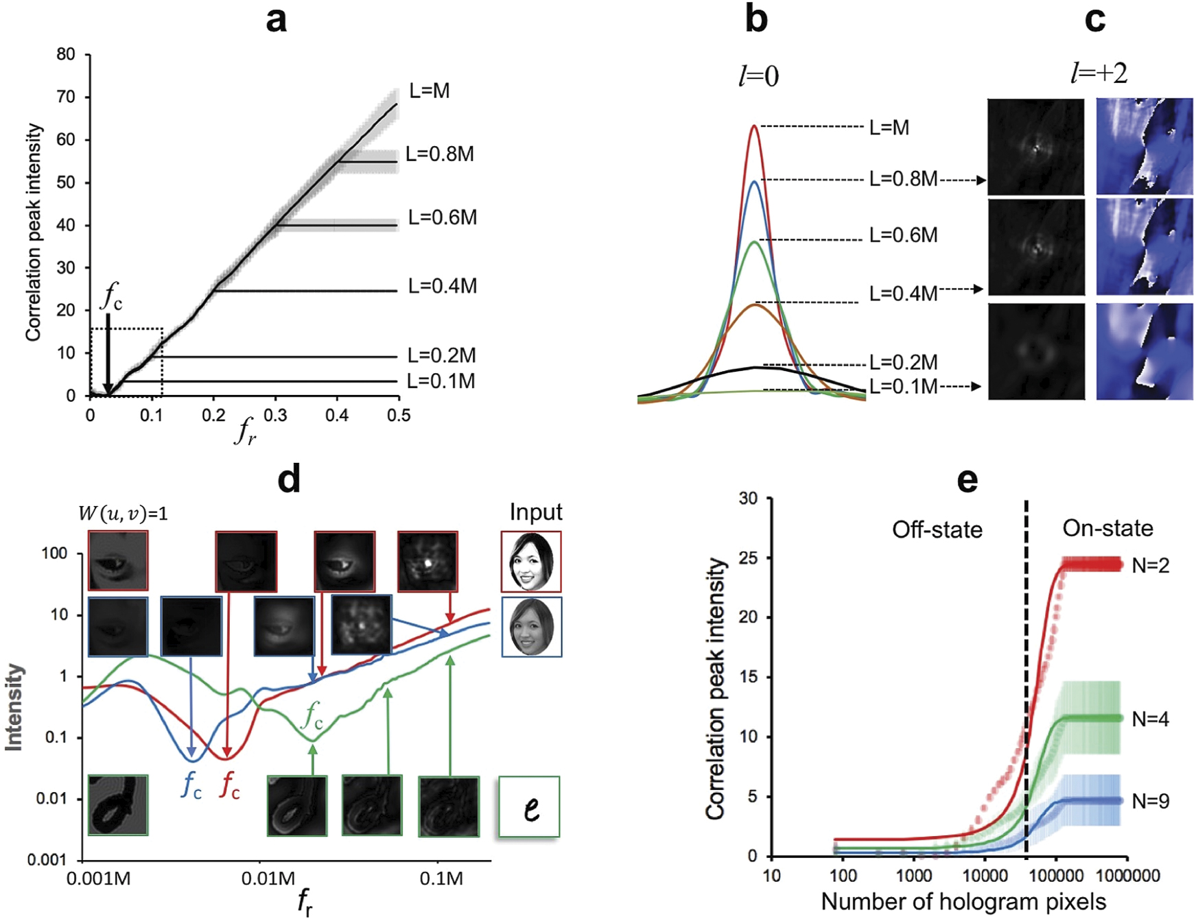
The finite transmission aperture of the SLM at the Fourier plane sets the maximum correlation peak intensity as well as the intensity distribution of the correlation peak at the output. The aperture effectively sets the numerical aperture of the optical system, where a small aperture results in a broader point spread function of the correlation peaks (figure 7(b)). It also affects the phase singularity when l ≠ 0. Figure 7(c) shows the intensity and phase distribution for l = +2 for different aperture diameters. Phase discontinuities for l ≠ 0 remain constant and independent of the system's numerical aperture.

The storage of spatial frequency information differentiates the correlation between NC and HC patterns. Figure 7(d) plots the output peak intensity as a function of f_r for a training set with N = 9 matched filters . Representative output intensity distributions are shown for three types of inputs: HC (red), NC (blue) and alphanumeric (green) patterns. Note that each pattern type has their respective $W\left(u,v\right)$'s calculated. At f_r = 0, the hologram at the Fourier plane is fully transmissive with no spatial phase modulaton and the output yields a conjugate image of the input. When f_r = f_c, the output produces an inverse intensity image, which sets the measured correlation peak intensity at minimum. From the plot, we can deduce that for f_r < f_c, the spatial frequency information stored in $\mathrm{arg}\left\{W\left(u,v\right)\right\}$ has minimal effect to produce an effective correlation peak. However, when f_r > f_c, a linear increase in the peak intensity indicates that pertinent spatial frequency information stored in the hologram results in effective correlation.

Plotting the effect of f_r on the correlation peak determines the pertinent spatial frequency information necessary to be stored in the hologram. Moreover, differences in f_c's indicate that the stored spatial frequency information within $W\left(u,v\right)$ is highly dependent on the pattern type. NC patterns yield an f_c closest to the optical axis , while alphanumeric patterns exhibit the highest f_c among the three image types. HC patterns result in a slightly higher f_c (compared to NC) thereby increasing the active area of stored phase signatures. Hence, increasing the contrast of the visual data allows for an increased storage of relevant phase signatures for effective identification and discrimination.

The activation function of the HoloPheuron can be probed by plotting the correlation peak intensity as a function of the total number of phase-shifting pixels within the active area of the hologram. Figure 7(e) plots the activation function of the HoloPheuron for different N and with fixed SLM size of L = 0.4 M. An OFF-state occurs when the number of active hologram pixels is not enough to provide effective correlation, which occurs when f_r < f_c. As the number of hologram pixels is increased (f_r > f_c), the HoloPheuron turns to ON-state and projects a correlation peak. Since the finite number of pixels in the hologram limits the correlation peak intensity, the peak remains constant when f_r exceeds the total area of the SLM contained within L × L. From the plot of the correlation peak versus the number of pixels, the activation function of the HoloPheuron can be fitted with a sigmoidal function (figure 7(e)).