Data efficiency and extrapolation trends in neural network interatomic potentials

The loss landscape $\ell$ of a NN can be visualized by evaluating the loss function $\mathcal{L}$ along a trajectory between two parameter sets θ and $\boldsymbol{\theta}^{^{\prime}}$. The simplest approach is to linearly interpolate the weights [43], choosing a scalar $t \in [0, 1]$ such that $\boldsymbol{\theta} (t) = (1 - t) \boldsymbol{\theta} + t \boldsymbol{\theta}^{^{\prime}}$. Then, the loss landscape $\ell$ for a model becomes

$$\begin{equation} \ell(t) = \mathcal{L} \left( \boldsymbol{\theta} (t) \right) = \mathcal{L} \left( (1 - t) \boldsymbol{\theta} + t \boldsymbol{\theta}^{^{\prime}} \right). \end{equation} \tag{ 1 }$$

In this work, the loss $\mathcal{L}$ is evaluated on the training set of the model with parameters θ on a given dataset.

In the absence of the reference weights $\boldsymbol{\theta}^{^{\prime}}$, the LL can be constructed by sampling a random vector δ in the parameter space and plotting the LL around θ as

$$\begin{equation} \ell(t; \boldsymbol{\delta}) = \mathcal{L} \left( \boldsymbol{\theta} + t \boldsymbol{\delta} \right), \end{equation} \tag{ 2 }$$

where the domain of t is appropriately chosen to span a neighborhood of θ . This notion can be extended to 2D LLs by taking two orthogonal vectors $\boldsymbol{\delta}_1, \boldsymbol{\delta}_2$ such that

$$\begin{equation} \ell(t_1, t_2; \boldsymbol{\delta}_1, \boldsymbol{\delta}_2) = \mathcal{L} \left( \boldsymbol{\theta} + t_1 \boldsymbol{\delta}_1 + t_2 \boldsymbol{\delta}_2 \right), \end{equation} \tag{ 3 }$$

with scalars $t_1, t_2$ chosen to span a (two-dimensional) neighborhood of θ . These approaches have been used to study the LLs of NN classifiers in image datasets, interpolate between sets of classifiers, and explore the loss function around degenerate minima [47, 49–51].

One challenge when analyzing LLs is comparing different models according to their parameters. Because activation functions such as ReLU allow for scale-invariance of NN weights, especially when coupled with batch normalization techniques, the magnitude of the vector δ is not transferable from model to model. This prevents a fair comparison of LLs, curvatures, and sharpness metrics. To account for this, we use the filter normalization technique proposed by Li et al [44]. Therein, each random vector δ is normalized by the scale of each filter i, in each layer j of the NN, i.e.

$$\begin{equation} \bar{\boldsymbol{\delta}}^{(i,j)} = \frac{\boldsymbol{\delta}^{(i,j)}}{\lVert \boldsymbol{\delta}^{(i,j)} \rVert} \lVert \boldsymbol{\theta}^{(i,j)} \rVert, \end{equation} \tag{ 4 }$$

where $\lVert . \rVert$ is the Frobenius norm. Then, the LL is plotted according to the filter-normalized vector $\bar{\boldsymbol{\delta}}$,

$$\begin{equation} \ell(t; \bar{\boldsymbol{\delta}}) = \mathcal{L} \left( \boldsymbol{\theta} + t \bar{\boldsymbol{\delta}} \right), \end{equation} \tag{ 5 }$$

and analogously for 2D LLs.

Although informative, sampling LLs can have cost comparable to training the NN, since evaluating the loss for each interpolated weight in each direction is similar to one training epoch. Depending on the number of parameters and directions $\boldsymbol{\delta}_n$ under analysis, the loss may be evaluated over the entire training dataset a large number of times.

Despite the usefulness of visualizing loss landscapes, comparing them beyond qualitative insights requires figures of merit to differentiate them. The most commonly used metric in the field is the curvature of the LL [42], which is related to the magnitude of the eigenvalues of the loss Hessian. Although informative, the Hessian is a local property and cannot fully capture 'valley-like' degeneracies in loss landscapes. Furthermore, computing the full Hessian for a system with millions of training parameters would be intractable. Thus, alternative metrics to compare LLs are required.

In the case of NNIPs, which are often trained to both energies and forces, two LLs are obtained per model, one for each target value. Although they cannot be completely disentangled, both LLs should be compared simultaneously to assess model performance. To derive one of such metrics, we propose the use of 'loss entropy' [41, 52] to quantify loss flatness around optimized minima. Although variations of this quantity have been proposed, we use the formula

$$\begin{equation} S(T) = k \log \left[ \sum_{t} \exp \left( \frac{-\bar{\ell} \left( t \right)}{kT} \right) \right], \end{equation} \tag{ 6 }$$

where S is the entropy of the loss landscape $\bar{\ell} (t)$ computed with respect to energy or forces and averaged over N orthogonal, filter-normalized weight displacements,

$$\begin{equation} \bar{\ell} \left( t \right) = \frac{1}{N} \sum_n \ell (t; \bar{\boldsymbol{\delta}}_n) \end{equation} \tag{ 7 }$$

and kT is a weighting parameter that quantifies the 'flatness' of the LL with respect to a certain acceptable threshold of training loss. This is similar to distributions of microstates accessible at a given 'temperature,' and ensures that low-loss states contribute to a much larger entropy than high-loss states.

As the entropy of the LL of a NNIP takes into account both energy and forces losses, we adopt a strategy similar to the one used during training of the NNs by balancing energy and forces losses with a weighted sum,

$$\begin{equation} S = \alpha S_E(T_E) + (1 - \alpha) S_F (T_F), \end{equation} \tag{ 8 }$$

where α is a dimensionless parameter between 0 and 1 that weights the entropy of the energy loss (S_E ) and forces loss (S_F ). As these losses have different units, they have to be computed with different normalization parameters $k_E T_E$ and $k_F T_F$, each of which takes into account 'thermal randomness' of the training loss. For simplicity, in this work, we adopt k = 1 as a dimensionless parameter, and assign the adequate units to the 'thermal error' for better interpretability of the loss entropy.

NequIP [27] is an equivariant NNIP that uses Clebsch–Gordon transformations and spherical harmonics to incorporate equivariance in the model. NequIP demonstrates state-of-the-art accuracy in several datasets, data efficiency, and has been employed to simulate a variety of organic and inorganic systems.

    MACE [29] is an equivariant NNIP that uses higher-order messages to efficiently embed information beyond two-body interactions in traditional MPNNs. The model demonstrates state-of-the-art performance in a variety of benchmarks, faster learning, and competitive computational cost.

    Other NNIPs proposed recently and not benchmarked in this study include Allegro [30], GemNet [53], DimeNet [54], HIP-NN [55], NewtonNet [56], BOTNet [28], SchNet [57], PaiNN [58], and others [18, 20, 26, 59].

    Training details are provided in appendix A in the supporting information.

    The 3BPA dataset [32] under study in this work was chosen due to its previous use in the literature for benchmarking NNIP models in extrapolation behavior [28–30]. The benchmark involves training models on low-temperature samples and evaluating their performance on held-out samples from high-temperature simulations. Distributions of energies and forces of the 3BPA dataset are shown in D.1 in the supporting information, figure S2. Additional results using the ANI-Al dataset [60] be found in appendix D.2 in the supporting information.

Molecular dynamics simulations were performed for the 3BPA molecule using each of the models under study. In total, 30 trajectories were performed per model to obtain better statistics of their production behavior. Simulations were performed in the NVT ensemble using the Berendsen thermostat [61] implemented in ASE [62]. The initial configuration used for the simulation was chosen to be the ground state of the 3BPA molecule. The simulation was performed at 1600 K and a timestep of 1 fs to force the models to evaluate configurations outside of their training set (300 K samples) and beyond those quantified by the test set errors (1200 K samples). The time constant of the Berendsen thermostat was chosen to be 250 fs. The simulation was performed for 6 ps for all models. This time length was sufficient to ensure the temperature was equilibrated and remained at 1600 K for about 4 ps (see figure S8).

MD trajectories were considered unphysical if the distance between bonded atoms increased above 2 Å. This bond rupture was the main source of failure observed in the trajectories, and thus is the only one considered in this work.

When comparing NNIPs, metrics of interest typically include errors in predicting forces and energies of a test dataset, and are appropriately used as baselines for assessing model quality. However, accuracy metrics are not necessarily predictive of extrapolation power [33]. A simple test to consider when analyzing NNIP extrapolation is whether NNIPs can learn a PES despite being trained on noisy data. Although this test does not measure extrapolation to out-of-distribution data, it verifies whether models are expected to overfit to corrupted training data, which would lower their robust generalization power. For example, NN-based classifiers can overfit to random labels in image datasets or to completely random inputs [63], even in architectures with good generalization error that are designed to prevent overfitting. Most NNIPs have enough parameters to memorize the training data, but standard regularization and architectural choices can curb overfitting in NNIPs, leading to lower generalization errors.

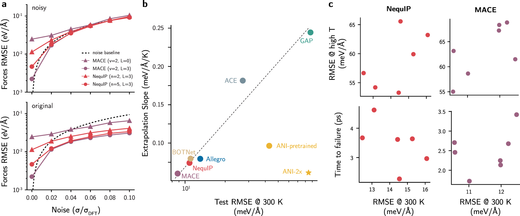
To test this hypothesis, we trained four different NNIPs to the 3BPA dataset and analyzed their training error. Following the lead from the deep learning literature [63], we then gradually corrupted the labels of the training set by adding a random sample from $\mathcal{N}(0, \sigma \cdot \sigma_{\textrm{DFT}})$ to the true forces, where σ_DFT is the standard deviation in the distribution of forces for the dataset obtained with density functional theory (DFT) (see appendix D.1 in the supporting information), and σ is a scalar ranging from 0.0 to 0.1. In principle, NN regressors with arbitrary levels of expressivity (or absent regularization) could achieve low training error even in these noisy PESes. Figure 1(a) shows the error for NNIPs trained to the 3BPA dataset with corrupted forces, and tested on the original, un-corrupted data. When the forces are not corrupted, models exhibit reasonable training errors lower than 40 meV Å⁻¹, as expected by their nominal performances in energy prediction [27, 29]. However, even small amounts of noise in the forces prevent the noisy dataset from being memorized with high accuracy, with the training loss plateauing instead of tending to zero. The ability of the models to predict the noisy forces saturates at the limit of the noise, indicating that these NNIPs do not memorize the high-frequency labels. On the other hand, when the test error of the models trained with corrupted labels is computed with respect to the uncorrupted dataset, the error is substantially smaller than the noise baseline (see the 'original' panel of figure 1(a)). Thus, the NNIPs under analysis are able to learn the underlying PES in the 3BPA dataset despite the added noise.

Zoom In Zoom Out Reset image size

Contrary to the overfitting hypothesis, these results suggest that data regularization in the training set may help NNIPs to 'denoise' the data. To understand this effect, we demonstrate in appendix B how data redundancy can downplay the effect of external noise in a toy system. Figure S1 shows how a large number of training points can counterbalance the effect of external noise when predicting the original, non-noisy data for the case of linear regressor models. In this case, the model averages out the noise and recovers the true function even at high levels of added noise. On the other hand, at the low-data regime, the regression model is unable to recover the true function, and its error quickly grows. Although the results from the linear model may not directly translate to the case of NNs, figure 1(a) shows that, to an extent, NNIPs are able to 'denoise' energies from the dataset due to architectural, training, or implicit data regularization.

To verify if this behavior was specific to the 3BPA dataset or could generalize to other datasets, we corrupted the energies or forces of the ANI-Al dataset and trained different models on the noisy values (see appendix D.2 in the supporting information), obtaining similar results even when only energies were considered. As the ANI-Al example exhibited even better results than the 3BPA, we tested whether a drastic increase in the injected noise could still be denoised by the NNIPs under study. Following the results of figure S1, we trained the two NNIP architectures under study to PESes with energy noises up to twenty times higher than those in figure 1(see figure S12), and up to twice the standard deviation of the original dataset distribution of the ANI-Al dataset. Although the distribution of per-atom energies shows that the noisy PES is completely different than the original one (figures S12(b) and (c)), all models succeeded in modeling the underlying PES below the error baseline (figure S12). As also illustrated by the toy example, the performance of the models degrades as extremely large amounts of noise are added. Nonetheless, errors with respect to the non-noisy dataset are remarkably low considering the corruption baselines.

The toy example from appendix B in the supporting information can be considered an upper bound of the 'dataset denoising' ability, given that a functional form of the inputs is known and the model could, in principle, fit perfectly to the data. As the trends of NNIPs trained on the 3BPA or ANI-Al potential approach this behavior, it can be concluded that the two NNIP architectures are able to 'denoise' the external noise added to the datasets, possibly due to data redundancy. As generalization tests assume the model is being tested on unseen data, it is not clear whether the accuracy reflects the quality of the model predictions or simply their ability to reproduce local environments existing in the training data. This is particularly important in the high-data regime, when the test dataset may be correlated to the train dataset in non-obvious ways.

To bypass the data correlation problem, alternative strategies were proposed to measure generalization power, including separating train-test splits according to sampling temperature, as is the case of the 3BPA dataset [32]. While testing a model on held-out samples from high-temperature simulations is typically considered an independent evaluation of its performance, we have found that extrapolation errors are correlated with low-temperature test errors across various model architectures. This is performed by fitting a linear model to the errors on the 3BPA testing sets at 300, 600, and 1200 K from the literature [28–30] (see figure S3), then using the slope of the fitted line as the associated metric. Figure 1(b) shows that all the models that were trained only to 3BPA frames at 300 K follow an approximate linear scaling relation between the extrapolation slope and the log of the low-temperature errors. This correlation between the low- and high-temperature data does not strictly preclude the use of the 3BPA dataset for assessing a fitted model's extrapolation abilities, as the extrapolation slope represents how much the accuracy of a given model degrades as the sampling temperature increases. Nevertheless, it suggests that data and model regularization effects may be enforcing extrapolation trends in wide error ranges. For example, a model like ACE [22, 28] is known to provide functional forms that aid extrapolation beyond the training data [32]. Despite this, the ACE model for 3BPA follows the same trends of more complex message-passing NNs. In fact, the generalization slopes are correlated to their low-temperature error regardless of significant architectural differences. This indicates that, for this benchmark, the RMSEs at higher temperatures can be estimated from the test error at 300 K even without evaluating the model at the other test sets.

The exceptions to this rule are the two ANI models ('ANI-2x' and 'ANI-pretrained'), which were pre-trained to the 8.9 million configurations from the ANI-2x dataset [64]. As seen in other fields of deep learning [65], the pre-trained models extrapolate better than all other models, though fine-tuning on 3BPA ('ANI-pretrained') leads to slightly worse extrapolation slope. These results suggest that: (1) more diverse datasets may be required for assessing the extrapolation and generalization capacity of a model; and (2) pre-training on large datasets may be required to create universal NNIPs [66], given that pre-trained ANI models were able to escape the scaling relation seen in figure 1(b).

Although the scaling relation can estimate the extrapolation slope within reasonable bounds, it is unable to recover trends within the same architecture in the low-error regime. As best-performing models often have differences of force errors smaller than 5 meV Å⁻¹ in the 300 K test set, their extrapolation behavior may not be accurately recovered from the scaling relation due to the statistical noise in the measurements. Indeed, figure 1(c) shows the correlation between the forces RMSE computed on the 300 K split and all splits (300, 600, and 1200 K, 'high T') for several NequIP and MACE models with different hyperparameters and training methods (see tables S3 and S6), but similar testing error at the 300 K split. Although there is a positive correlation between the two RMSE metrics, the dispersion of points indicates that models with nearly the same RMSE for the 300 K data split show discrepancies in error above 10 meV Å⁻¹ when all splits are taken into account.

This scenario is aggravated when MD simulations are used to test the extrapolation power of the NNIPs, which may exhibit higher diversity of configurations than those used to compute the extrapolation slopes. When measuring the average simulation times for each of the models (see Methods), no clear correlation is obtained between the error on the 300 K split of 3BPA and the average (physically meaningful) simulation length (figure 1(c)). This motivates the creation of a metric that captures robustness trends in NNIPs.

Beyond data regularization, architectural and training choices strongly influence generalization ability of NN models. Relevant aspects include model initialization, hyperparameter optimization, choice of optimizer, batch sizes, and many others. Although the process of training NNs strongly affects their extrapolation behavior, good NN models systematically outperform their counterparts by optimizing to better local minima in the LL [67]. Thus, using these insights, we propose that loss landscapes of NNIP models can predict their generalization ability towards unseen data despite using only the training data. Correlations between robust generalization and loss sharpness have been observed for other NN models in the literature [41, 42], but not yet explored in the context of NNIPs.

To first verify if qualitative insights could be derived from LLs in the context of NNIPs, we investigated the behavior of the loss function around the optimized minima of the NNIP models trained to the non-noisy 3BPA dataset. To ensure the LL visualizations were statistically meaningful, we sampled 20 different orthogonal directions for each set of parameters and models, and interpolated them using the filter-normalized method described in the Methods (see also figure 2(a)). Then, we compared the LLs of the NNIP models using 2D visualizations, as often done for NN classifiers [44]. Qualitative inspection of the 2D LLs in figure 2(b) reveals the presence of weight degeneracies in the prediction of energies in models (see also figure S14 for another example in the ANI-Al dataset). This 'valley-like' landscape represents a subspace of weights leading to similar accuracy in energy [68], and reflects the interplay between energy and forces during training. These results agree with the literature regarding LLs of over-parameterized models [69], as well as the notion that physical systems often result in so-called 'sloppy' models [70, 71], and can improve trainability and interpolation [72].

Zoom In Zoom Out Reset image size

Qualitative analysis of LLs also explain other factors typically found as heuristics of NNIP training. For example, the energy/forces coefficients in the final loss are often defined from hyperparameter optimization [27, 73] and have ratios varying from 1:10 to 1:100 for energy:forces losses, but the success of higher force coefficients can be justified using LLs. In figure 2(b), we show how a higher weight on force losses leads to LLs with less saddle points around the optimized minima, thus favoring training. Although energy and forces are related and completely disentangling their effects is not achievable, the interpolation in figure 2(b) shows how mixing both can lead to better optimization landscapes for NNIPs. Based on these results, an effective training regimen would start with a relatively large weight for forces loss for a fast (and smoother) optimization of forces. Once the force errors are reasonably converged, the weight can be decreased until a desired threshold in energy errors is achieved. Similar strategies with WC and scheduling—e.g. starting with an energy:force loss weighting of 1:10, but then switch to 1000:1 in the later stages of training—can also be effective.

One limitation of visualizations of the high-dimensional LL is that different directions in weight perturbation may lead to similar losses. This results in only slight variations in landscape topography with different random directions, as noted in figure 2. This may be related to the dominance of specific layers of the model in the filter normalization technique. Figure S13 shows how the distribution of weights is non-uniform, suggesting that some layers have higher sensitivity to weight perturbation than others. As the filter normalization displaces the model weights along random directions with magnitude proportional to the norm of each filter and layer, parameters with higher weights may influence certain regions of the loss landscapes. An exception to this point is when the parameters are intertwined with functions embedded in the architecture, such as the trainable Bessel functions in NequIP. As shown in figure S6, freezing certain high-magnitude weights when generating the LLs can help flatten the landscape and remove spurious minima, emphasizing the importance of proper regularization and training regimen taking these effects into account (e.g. separate learning rates for certain layers in the model).

In the context of NNIPs, robust generalization has important ramifications in two distinct areas: the stability of the model in production (e.g. MD simulations), and its data efficiency during training. To probe the first of these features, we trained NequIP models using various choices of model architecture and optimization techniques (see table S1) in the low-temperature split of the 3BPA dataset. Then, we performed MD simulations in the NVT ensemble with a high temperature of 1600 K (see Methods) to ensure all models were extrapolating well beyond their training split. Furthermore, as the 3BPA benchmark already provides geometries sampled from simulations up to 1200 K, the MD trajectories at 1600 K could provide information beyond the 1200 K splits provided by the dataset. For each model in the study, 30 MD trajectories were simulated to obtain reasonable statistics on the model behavior, with simulation timelengths of up to 6 ps and a timestep of 1 fs. In principle, a model's ability to extrapolate beyond the training set can be assessed by the number of trajectories that behave in a physical way [38], as well as the average trajectory length until the model fails to extrapolate (see Methods).

Using the results from MD simulations, we investigate whether LLs can predict the extrapolation behavior and trajectory stability of models. While the test performance at low-temperature samples is unable to perform such predictions, the test error at high-temperature samples is still expected to be a reasonable predictor of such stability. Nevertheless, whereas high-temperature samples are available in the 3BPA dataset, out-of-domain data is often not available for an arbitrary material system. In addition to being expensive to generate using ground-truth methods, sampling new configurations is rarely performed in an exhaustive way. Thus, the major advantage of extrapolation tests based on LLs is their reliance only on the training dataset. To quantify the sharpness of the LLs [42], we compute the loss entropy as described in the Methods, with T_E and T_F taken to be reasonable 'room temperature' values of the energy/force RMSEs, respectively ($T_E = 4$ meV/atom, $T_F = 40$ meV Å⁻¹). The weight α was set to 0.2 to resemble the higher force weighting used during training without ignoring the contributions of energy LLs in model stability. A full sensitivity analysis of S with respect to these parameters showed that results remained consistent around these error ranges, as long as unreasonable temperature values were not used (see figure S4).

The relationship between the model/training parameters, the MD stability, and LLs entropy are shown in figure 3(see also table S2). The analysis is grouped into four experiments (columns in figure 3) to isolate the effects of specific portions of the training procedure and model architecture, thus uncovering useful trends for NNIP practitioners. For example, considering only the distributions of time to failure from MD simulations in figure 3(b), it can be seen that rescaling the energies predicted by the model (models 'no rescaling' vs. 'rescaling') greatly improves the stability of the model, especially when the Bessel weights used by the radial basis are trainable. This behavior is reflected in the energy and forces LLs (figure 3(a)), with the LL of the model without rescaling showing considerable sharpness compared to the models using rescaled energies. Quantitative trends are also obtained when the loss entropy and test RMSE at all splits in the 3BPA dataset are computed (figure 3(c), first column, and table S3). Models with rescaling showed higher average simulation time with physical trajectories, as well as increased entropy and lower forces RMSE.

Zoom In Zoom Out Reset image size

When comparing how the training regime can change the extrapolation behavior of NequIP, the results show that the AMSGrad variant of the Adam optimizer [74] leads to consistent improvements in the model extrapolation both for the two-layer and the five-layer model (figure 3(b), second and third column) compared to the baseline, which does not use AMSGrad. The improvements of simulation quality are particularly pronounced in the five-layer models, where the model trained using AMSGrad shows significant improvements in simulation stability compared to the baseline despite not using trainable Bessel functions (table S1). On the other hand, the exponential moving average (EMA) appears to degrade the extrapolation performance of the NNIPs, often leading to sharper LLs if used in isolation and with constant learning rates. These trends are reflected in the extrapolation metrics (figure 3(c)). Although the loss entropy underperforms compared to the forces RMSE in the case of the two-layer models, the trend is correctly captured for the five-layer model, where the model trained with AMSGrad showed both higher loss entropy and higher MD stability.

Finally, NequIP models can be compared according to the number of message-passing layers. Using a fixed training regime, a higher number of layers showed pronounced improvement both in the stable simulation time (figure 3(b)), as well as in the forces RMSE and loss entropy (figure 3(c)), with the trend remaining consistent across these models. Interestingly, the improvement in loss entropy for the 5-layer model is reflected mostly in the energy LL rather than the force LL (figure 3(a)). Although only forces are required when integrating the equations of motion in the NVT ensemble during an MD simulation, the wider minima in energy LL reflects the model's higher generalization capacity towards forces obtained by differentiating the energy through the NNIP architecture. This phenomenon can be explained by recognizing that the out-of-domain data often results in a horizontally shifted version of the loss landscape [47]. To explain this effect, we computed the LL of NequIP models with respect to the test sets instead of the training set (see figure S5). As expected, the test LLs show higher errors compared to the train LL, as seen in the vertical shift of the curves. However, while the forces LL only undergo a vertical shift, test energy LLs also undergo a horizontal shift, indicating that the optimal model for the training set is not necessarily optimal for predicting energies of the testing sets. Furthermore, as the forces loss is often derived from the energy in NNIPs, the propagation of these mismatches may be responsible for degradation in extrapolation performance. Thus, in general, the results in figure 3 show that architectures and optimization strategies which result in loss landscapes with higher entropy (i.e. flatter landscapes) tend to demonstrate improved stability in MD simulations that sample out-of-domain configurations.

To confirm that the results could be extended beyond NequIP, we performed a similar study using the MACE framework. Given the differences in architecture and available code, MACE has different hyperparameters and optimizer choices than NequIP (see table S4). Nevertheless, a similar study for MACE reproduces the trends seen for NequIP, as shown in figure 4.

Zoom In Zoom Out Reset image size

As seen in the case of NequIP, model stability can be greatly improved by using rescaling and AMSGrad. Also for MACE, EMA appears to lower the time-to-failure if used in isolation, with similar trends in out-of-domain RMSE, loss entropy, and MD stability seen in the NequIP case (figure 4). In addition, we also explored the effects of stochastic weight averaging (SWA) [75] and WC (column 2 of figure 4) implemented in the MACE code. Consistent with results from the use of SWA for image classification tasks [75], SWA + WC is shown to improve model generalizability, leading to higher simulation times and flatter loss landscapes. Interestingly, the model trained with SWA + WC exhibits similar force RMSE in high-temperature samples compared to the baseline, but a higher loss entropy and higher MD stability (figure 4(c)). As SWA flattens the loss landscape by design [75], implementing this strategy in other NNIP models may be a low-cost modification for improving the generalization capacity of different architectures. The use of WC can also help the optimization process (see previous results) and lead to better energy landscapes overall.

For the MACE study, we also analyzed the relationship between the bond order of the model (column 4) and its stability in production MD simulations. In this case, the loss entropy recovers the trend in MD stability better than the forces RMSE (figure 4(c), column 4). Interestingly, despite the higher errors of the $v = 1, L = 3$ model compared to its $v = 2, L = 3$ counterpart, the former still exhibits a higher average time to failure. This observation can be traced back to the flatter energy LL (figure 4(a), column 4), as also seen in the case of NequIP.

Finally, the models were compared according to the symmetry order of the edge features (column 3). In general, increasing the value of L from L = 0 to L = 2 led to more stable simulations, although the model with L = 3 shows a degradation of the production behavior. Nevertheless, the LLs do not follow the expected trends explained so far in this work. We believe the filter normalization technique discussed in the Methods cannot provide comparable LLs upon changes of L in MACE. As this parameter affects the tensor order of some model components [29], the number of parameters in these particular filters grows with $\mathcal{O}(N^L)$, which may be affecting the filter normalization. In contrast, adding message-passing layers with similar numbers of parameters, as in NequIP, allows the filter normalization technique to create comparable loss landscapes. This result shows some limitations of the loss entropy when comparing models with different architectures or hyperparameters, and may require different strategies for computing them in the future.

Since extrapolation power and data efficiency are conceptually related, a natural extension of these results is to verify whether the loss landscape entropy can also be used to predict the data efficiency of a model during training. As with many other applications of deep learning, generating training data is often one of the most costly steps in the development process. Especially considering the 'denoising' effects of NNIPs demonstrated in this work, identifying training techniques and model architectures that lead to more data-efficient training has the potential to greatly reduce the computational cost of building new NNIPs.

To test whether loss entropy can predict the data efficiency of models, we computed the learning curves for NequIP and MACE models with the hyperparameters selected in the previous sections. This is achieved by training models with the specified training parameters and architectures to the same subsets of the 3BPA training set using only 25, 125, 250, or 500 samples from the 300 K split (tables S3 and S6). Following previous work [27], the slopes of the learning curves were then computed by fitting the line $\log{n} = m \log$ ${\varepsilon} + b$ to the number of training samples n and the force RMSEs ε calculated using all test splits (300, 600, and 1200 K), and comparing the slopes m. Consistent with the results from the previous sections (combined in figures 5(a) and (b)), the high-temperature force RMSEs (i.e. the points from the learning curves using n = 500) are good predictors of the learning curve slope. In addition, figures 5(c) and (d) show that the loss entropy also has a high correlation with the slope of the learning curve despite being computed using only the training set. As discussed previously, these correlations are less explicit for the case of MACE models, and thus show that none of the metrics is truly universal for predicting stability in simulations and learning curve slopes. Nevertheless, these results further demonstrate that loss landscapes provide information on the extrapolation behavior of NNIPs despite being derived only from the training set.

Zoom In Zoom Out Reset image size