
Abstract
Graph neural networks (GNNs) have been employed in materials research to predict physical and functional properties, and have achieved superior performance in several application domains over prior machine learning approaches. Recent studies incorporate features of increasing complexity such as Gaussian radial functions, plane wave functions, and angular terms to augment the neural network models, with the expectation that these features are critical for achieving a high performance. Here, we propose a GNN that adopts edge convolution where hidden edge features evolve during training and extensive attention mechanisms, and operates on simple graphs with atoms as nodes and distances between them as edges. As a result, the same model can be used for very different tasks as no other domain-specific features are used. With a model that uses no feature engineering, we achieve performance comparable with state-of-the-art models with elaborate features for formation energy and band gap prediction with standard benchmarks; we achieve even better performance when the dataset size increases. Although some domain-specific datasets still require hand-crafted features to achieve state-of-the-art results, our selected architecture choices greatly reduce the need for elaborate feature engineering and still maintain predictive power in comparison.
Export citation and abstract BibTeX RIS

Original content from this work may be used under the terms of the Creative Commons Attribution 4.0 license. Any further distribution of this work must maintain attribution to the author(s) and the title of the work, journal citation and DOI.
1. Introduction
Designing new materials is a major research challenge given its technical complexity and potential scientific and social impact. Experimental screening is impractical due to its high demand in human time and resources, and computational screening based on physics-based simulations remains challenging due to its computational complexity and cost. An AI-augmented approach where machine learning techniques are leveraged to learn from prior data and propose insights can help accelerate this process.
Materials can be naturally represented as graphs with atoms as nodes and distances/bonds between them as edges, and graph neural networks (GNNs) learn to predict material properties from the atoms and their nearest-neighbor connections through graph convolutions. Many flavors of GNNs share the same basic pattern of graph convolution but differ in additional features and associated operations. Take GNNs for predicting quantum chemical properties of crystalline materials for example. The crystal graph convolutional neural network (CGCNN) [29] uses the distance between atoms in the crystal graph as edges encoded with a Gaussian radial basis. Improved CGCNN (iCGCNN) model [20] incorporates Voronoi connectivity, explicit 3-body correlations, and additional edge features from Voronoi polyhedral information. The Materials Graph Network (MEGNet) [3] introduces the option of incorporating additional temperature, pressure, and entropy as global state inputs. Orbital graph convolutional neural network (OGCNN) adds orbital–orbital interaction features and topological features to the convolution [13]. The directional message passing neural network (DimeNet) [15] incorporates directional information where angles are encoded as spherical Bessel functions and distances as radical basis functions. Cheng et al argue that many GNNs incorporate incomplete spatial geometrical information and propose additional geometric features in GeoCGNN for learning the complete local geometrical relationship between atoms [4]. Choudhary and DeCost propose an Atomistic Line GNN (ALIGNN) that performs message passing on not only interatomic bonds but also on a line graph that corresponds to additional bond angles [5].
The trend in current studies of GNNs for material research appears to incorporate increasingly sophisticated features. While intuitively physics-informed features may be helpful for a model's performance, they present two major practical issues. The first is the lack of canonical forms of GNNs due to the abundance of options with subtle differences, and as a result extensive domain knowledge is needed to justify these choices and a practitioner can easily be overwhelmed; and the second is that they go against the mantra of deep learning where the features are implicitly reconstructed through the sophisticated structures of neural networks, and these GNNs will likely not take full advantage of the datasets that is constantly being extended.
Instead of engineering extra elaborate features, we propose neural network architectures such as extensive attention mechanisms in GNNs for accurately predicting the properties of materials. Analogous to computer vision or machine translation, where feature engineering is rendered unnecessary by deep CNNs, we show it is possible to achieve similar or even better performance through sophisticated networks without feature engineering for property predictions. We evaluate the performance of our model with popular materials benchmarks for predicting quantum chemical properties such as formation energy and band gap. The inputs to our model are plain graphs with atoms as nodes and distances as edges without any other features or transformations, not even the popular Gaussian radial basis transformation used in many GNNs to represent the edge attributes. We show that for the widely benchmarked Material Project (MP) 1 June 2018 version (mp-06-01-2018), our model achieves equivalent or better performance with the state of the art models such as GeoCGNN and ALGNN. For a later and larger MP dataset (mp-05-13-2021), our model achieves even better performance than GeoCGNN and ALIGNN. Moreover, our model is much more robust to the presence and absence of features compared with other GNNs when there are enough training samples. As the importance of AI is universally recognized and more data is being collected, our model is an important step towards a common canonical form of GNN for material research. We also show that before the amount of data becomes abundant, domain insights and feature engineering can be helpful. Some recent studies propose architectures for encoding periodic structures, e.g. Matformer [30], and for achieving equivariance to rotations, translations, and permutations, e.g. TF networks [23] and Equiformer [17]. On one hand they employ modern sophisticated neural network architectures such as transformers in GNNs, and on the other hand, compared to our architectures, they still require special features such as Irreps features (e.g. Equiformer) and spherical harmonics (e.g. TF networks) or customized graph constructions (e.g. Matformer).
To further evaluate the generality of our model, in addition to quantum chemistry properties, we test it on predicting the  adsorption of metal–organic framework (MOF). Since the calculation of
  here does not utilize density function theory (DFT) calculations and in some cases does not depend significantly on the electronic structure of the material, engineered features utilized in prior GNNs for materials such as plane wave features in GeoCGNN should not be helpful. Our experiments reveal interesting findings. Currently, the best results achieved in prediction of
  adsorption are from classical machine learning models such as random forests or decision trees with many (over one hundred in this case) engineered features. To predict adsorption at low pressure, our model achieves better performance than prior approaches. At high pressure, our model achieves better performance for one dataset but not for the other. We investigate the cause of the behavior, and discuss the relationship between features and data size for GNNs. In fact, none of the GNNs (including our own) we study is able to beat the prior best machine learning method using decision trees with extensive features. This points to the limitations of current GNN designs for materials, and we propose future research directions in the architecture of GNNs.
2. Feature engineering in GNNs for materials
GNNs predicting material properties include node features that are usually an encoding of the atom species number (e.g. through one-hot encoding) and edge features representing the relationships among atoms (e.g. distances between them). The convolution computes the feature of a node using the features of its neighbors and the incident edges. The 'aggregation' of neighboring features is termed 'message passing'. Almost all GNNs since the introduction of DTNN [22] have a similar set up, and differ in the inclusion of additional features and transformations on them, and other operations beyond message passing.
We sample some of the popular edge features in literature. The first is the feature derived from Gaussian radial basis function  , and it is extensively used in GNNs for materials [4, 21, 25, 29]

where r is the distance between atoms, φ is a cut off function, βt
and µt
are the constant parameters of the  order. Radial basis functions are often used to approximate other functions, and as a kernel in support vector classification [2].
The Fourier–Bessel basis function is another transformation to encode spatial and chemical information as features. In DimeNet, it is shown that even utilizing the simplest wave function (the solution of Schrödinger equation under infinite sphere potential) can produce features that significantly improve the performance of the GNN model.
The 2D spherical Fourier–Bessel basis is given as

with c as the cutoff, jl and yl as the spherical Bessel functions of the first and second kind, zln the nth root of the l-order Bessel function, Yl the spherical harmonics, and α the angles between message embeddings.
Noting that plane waves are eigenfunctions of the Schrödinger equation with constant potential and form the natural basis in the nearly-free-electron approximation, Cheng et al use the following plane wave basis set of features in GeoCGNN [4] as well as the Gaussian radial basis features

with  ,
,  ,
,  , Ω as the volume of the crystal cell, k are the points in reciprocal space.
As is already apparent with this partial list of engineered edge features, the functions and transformations become increasingly complex and the insights are only possible with deep knowledge of specific domains such as quantum physics. On one hand, it is not surprising that these features are shown to help the model performance. On the other hand, they raise an important question from the modern deep learning perspective. That is, since these transformations all have closed-form mathematical formulas, and deep neural networks are universal function approximators, are there significant barriers for GNNs to implicitly construct these features? The answer to this question has serious implications for practitioners. If the models for material research do require elaborately engineered features for high performance, then for predicting different properties, there will not be a unified, canonical architecture as ResNet [10] for computer vision or Transformers [27] for natural language processing. Practitioners thus will have to invest significant efforts into the feature engineering step.
Our hypothesis is that with a capable enough model and large enough dataset, it is possible to learn material properties with GNNs without elaborate feature engineering.
3. Minimal-feature crystal GNN
To explore learning without elaborate feature engineering, we introduce our minimal-feature crystal GNN (MF-CGNN ). With MF-CGNN, the input graph is represented with atoms as nodes and distances between them as edges. The node feature is a simple one-hot vector encoding of the atom species number, and the edge feature is plain Euclidean distance without any further transformation.
In describing MF-CGNN we use the following notations. Let  denote an undirected graph with vertex (node) set V and edge set E.
  contains all atoms in a material and
  contains all edges representing connections between atoms i and j,
  . A feature vector vi
is associated with each node i and a feature vector
. A feature vector vi
is associated with each node i and a feature vector  is associated with each edge (i, j).
GNNs are characterized by convolutions to node features through message passing. For example, graph convolution network (GCN), one of the first GNNs, conducts convolutions as a localized first-order approximation of spectral graph as follows [14]

In equation (1),  denotes the hidden feature at node i at layer l. The hidden feature at layer l + 1,
  , is computed by aggregating hidden features of node i's neighbors
  ,
,  .
.  is a constant, bl
is the bias vector, and Wl
is the weight matrix; the latter two are parameters to be learned.
is a constant, bl
is the bias vector, and Wl
is the weight matrix; the latter two are parameters to be learned.
In comparison to equation (1), MF-CGNN introduces additional convolutions and mechanisms.
3.1. Convolution with edge features and for edge features
Due to the importance of edge features in material research, when computing hidden features, e.g.  , MF-CGNN convolves not only node features but also edge features. The convolution function
  uses the previous layer's features from node i's neighbors and from all edges incident to i as follows:

Here  is the set of features for all neighboring nodes to i. Similarly,
  is the set of features for edges incident to i. In the message-passing paradigm, node features as well as edge features are 'passed' to the neighbors for their feature computing. Here
  is a linear combination of all features involved with some nonlinear activation function.
MF-CGNN further emphasizes the importance of edge features by introducing a convolution for the edge features:

Similar to  ,
,  is a linear combination of features followed by a nonlinear activation. As now there is a hidden feature for edge e at each layer l, the node convolution in equation (2) becomes

In MF-CGNN a convolution layer produces two kinds of outputs, node features and edge features.
3.2. Attention in convolution
Attention [27] is a powerful mechanism that revolutionizes learning in many research areas. As its name suggests, attention in learning mimics its cognitive counterpart and captures dependence (both spacial and temporal) between parts of the input. Oftentimes multiple attention heads are used, and the attention function are learned simultaneously with the features [28].
Prior GNNs for materials, e.g. CGCNN and GeoCGNN, implement attention with a gated form as shown in equation (5)

here  is element-wise multiplication, σ is the Sigmoid function, g is a nonlinear activation function, and
  is the concatenation of vi
, vj
, and
is the concatenation of vi
, vj
, and  . Wc
and bc
are the convolution weight matrix and bias vector, and Ws
and bs
are the self-weight matrix and self-bias vector, respectively.
. Wc
and bc
are the convolution weight matrix and bias vector, and Ws
and bs
are the self-weight matrix and self-bias vector, respectively.
In MF-CGNN we adopt attention in the general form with Softmax as in GAT [28]. In addition, in computing the hidden feature of a node, MF-CGNN attends to features of the neighboring nodes as well as incident edges as shown in equation (6).

here Γ is the Softmax function. In computing  (and similarly
  ), MF-CGNN attends to the features of vj
and
), MF-CGNN attends to the features of vj
and  . The multi-head attention (with M heads) flavor of MF-CGNN is shown in equation (7).

where 
MF-CGNN also introduces attention to its pooling. Instead of simple averaging of attention outputs in equation (7), MF-CGNN uses attention to combine these outputs as well. The resulting node or edge feature benefits from a weighted contribution from each head. As expected, extensive attention mechanism and edge-oriented convolution can improve the learning performance of GNNs on inputs with engineered features such as Gaussian radial basis and plane wave basis for some tasks [7].
3.3. Attention in pooling
Pooling is necessary to derive a feature for the entire material from the features of individual nodes (and/or edges). MF-CGNN attends to each node (and/or edge) in pooling for the global feature s for the graph. Equation (8) shows the pooling from the node features (similarly, pooling can also be done on the edge features).

Here Γ is the Softmax function, L is the last layer of GNN convolution. As an example of self attention, f computes an input to Γ from  .
.
4. Prediction tasks and characteristics of the datasets and graph patterns
To demonstrate its advantages, we employ MF-CGNN to predict two sets of material properties. The first set is quantum chemical properties such as formation energy and band gap, with the ground truth computed from DFT calculations. DFT is a quantum mechanical method for solving the electronic structure of a material widely used in computational materials chemistry. The formation energy is a measure of the stability of a chemical compound defined as the difference between the total energy of the compound and the sum of the energies of its constituent elements. The band gap of a material is the energy difference between its highest occupied electronic energy level and the lowest unoccupied energy level. The second set is  adsorption, with the ground truth provided by physics-based GCMC simulations. The GCMC simulation consists of a series of steps in which 'Monte Carlo moves' are attempted. Suitable Monte Carlo moves include molecular translations, insertions, deletions, rotations and swaps. Moves that lower the energy are favored and those that increase the energy are accepted with a probability given by the Boltzmann distribution.
The  adsorption for each material was calculated at room temperature for high (16 bar) and low (0.15 bar) pressures, simulating adsorption and desorption conditions, respectively.
For formation energy and band gap prediction, we use the material project dataset (MP ) [12]. Unless noted otherwise, MP refers to the 13 May 2021 version. For  adsorption of MOFs, we use the CoRE-19 dataset (CoRE-19 ) [6] and the Boyd–Woo dataset (BW ) [1]. These datasets have different characteristics from the machine learning perspective. Table 1 summarizes key statistics, and provides some hints as to the performance of GNNs on these datasets.
Table 1. Characteristics of MP, CoRE-19, and BW datasets. Here min, max, and median are for the graph sizes (i.e. the number atoms in the material structures) in the dataset.
| Dataset | min # nodes | max # nodes | median # nodes | # structures | # unique elements |
|---|---|---|---|---|---|
| MP | 1 | 444 | 180 | ≈140 000 | 89 |
| CoRE-19 | 10 | 5750 | 290 | ≈10 000 | 77 |
| BW | 22 | 1244 | 122 | ≈20 000 | 16 |
Of all three, MP is the largest with roughly 140 000 structures, and the structure sizes (number of nodes in the graph) has the smallest range between 1 and 444. CoRE-19 is the smallest, yet it has a large span of structure sizes, between 10 and 5750. BW is in the middle, with structure sizes ranging between 22 and 1244. CoRE-19 and BW are built from existing Crystallographic Information File (CIF) databases [18]. CoRE-19 [6] contains approximately 10 000 MOF materials, while BW is a subset of the original BW-DB database [1] containing only approximately 20 000 MOFs. Modern deep learning tasks typically require big models to have enough expressive power to learn hidden features, and correspondingly need large enough datasets for training. For GNNs the larger the range of individual graph sizes the more challenging the problem can be. The diversity of the datasets, a simple and straightforward measure of which is the amount of unique elements, also plays a role. The more diverse the dataset, the more data is needed for learning. Table 1 suggests MF-CGNN may perform better with MP, and may face the biggest challenge from CoRE-19.
Increasing the predictive capacity of GNNs is primarily accomplished through more convolution layers. However, typical GNNs with very deep layers suffers from over-smoothing. That is, node features become homogeneous and lose their distinguishing power [19]. At the same time, the GNNs need enough layers to be able to capture the impact of a node's remote neighbors. Recall that with GNNs, the feature of a node is influenced by the features of other nodes in its neighborhood. The number of layers determines the size of a neighborhood that contributes to a node's feature. If a node's neighborhood is to cover a significant portion or the entirety of the graph, the number of layers of the GNNs will be directly related to the diameters (or radii) of the graphs.
We compute the diameters of graphs generated for MP, CoRE-19, and BW. We note that for a periodic structure there may not be a well-defined diameter. The diameter we consider here is a concept in classical graph algorithms and for the graphs constructed for the unit cells. The diameter of a graph is the length of the shortest path between the two most distant nodes in the graph, i.e. the longest shortest path between any two vertices. Diameter is important for GNNs as it can determine the number of GNN layers necessary to propagate information in message passing from one node to other nodes. As commonly done in prior studies, the graphs are generated with a maximum of 12 neighbors and cut-off 8 Å.
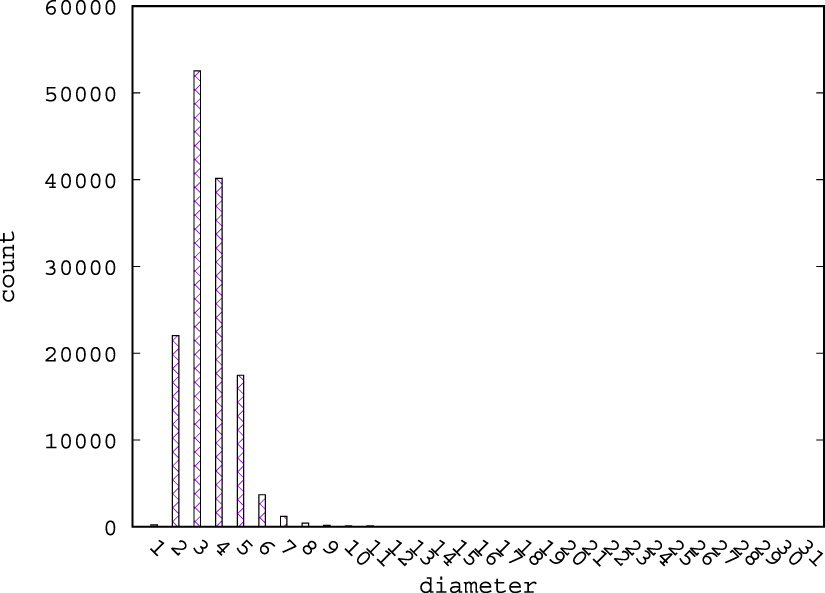
Figures 1–3 show the distribution of diameters for structures in MP, CoRE-19, and BW, respectively. In these figures, we ignore graphs that are not connected. For MP, the maximum diameter is 22, and the minimum diameter is 2. Most of the graphs have a diameter no larger than 6. For CoRE-19 and BW, most structures have diameters smaller than 8. A GNN with 4 layers can capture the contribution to a node's feature by all other nodes for most graphs. The diameter distribution for CoRE-19 has a longer tail than BW and MP, and this suggests that MF-CGNN may perform better for MP than BW and CoRE-19, due to the abundance of data and similarities among graph structures. We expect CoRE-19 to be more challenging, due to its relative small dataset size and large variance in graph structures.

Figure 1. Histogram of diameters for MP.
Download figure:
Standard image High-resolution image
Figure 2. Histogram of diameters for CoRE-19.
Download figure:
Standard image High-resolution image
Figure 3. Histogram of diameters for BW.
Download figure:
Standard image High-resolution image5. Results
We compare MF-CGNN with prior GNNs and other machine learning methods that leverage extensively engineered features motivated by physical insights. For quantum chemical properties prediction, prior GNNs have achieved excellent performance. In addition to showing that MF-CGNN achieves similar or even better performance without the need of feature engineering, we study the impact of dataset characteristics (primarily size) on performance. For  adsorption, the best prior implementation is not a GNN, but a classical machine learning method with over one hundred features. We show the good performance of MF-CGNN and also point out limitations of current GNNs for such tasks.
5.1. Quantum chemical properties prediction
Several studies have developed and evaluated GNNs for predicting quantum chemical properties such as formation energy and band gap. Most recent GNNs for material property prediction incorporate additional features than those present in the original CIF files. Among these, GeoCGNN [4] and ALIGNN [5] are among the latest that achieve state-of-the-art performance, and attribute explicitly the performance gain in comparison with prior ones such as CGCNN, MEGNet [3], iCGCNN [20] and etc to the inclusion of additional geometric features.
For comparison purposes, we use the identical 06-01-2018 version of MP (mp-06-01-2018) as in prior studies which contains about 70 000 samples. We use a train-validation-test split of 60 000–5000–4239 as used by the SchNet, MEGNet and ALIGNN papers. We use a 4-layer MF-CGNN. The original input features are one-hot encoding vectors for the atomic species numbers. These vectors are first embedded into 192 dimensional vectors before graph convolution. All hidden features for the vertices and edges are 128 and 64 dimensional, respectively. We use 3 attention heads and ReLU for activation. A one-layer multilayer perceptron is used to predict the target properties. The fully connected layers are  . The optimizer used is Adam with learning rate 10−3 and weight decay
  . We train for 300 epochs with the training set, and report the test accuracy on the test set with the model that achieved the best validation accuracy on the validation set. We note that the hyper-parameters used in MF-CGNN are almost identical to those of GeoCGNN. The reported results are averaged among three runs and we note there is very minimal variance between runs. The results are shown in table 2.
Table 2. Predicting formation energy and band gap with various GNN implementations using mp-06-01-2018.
| Property | Unit | CGCNN | MEGNet | SchNet | ALIGNN | GeoCGNN | MF-CGNN |
|---|---|---|---|---|---|---|---|
| Ef | eV at.−1 | 0.039 | 0.028 | 0.035 | 0.022 | 0.024 | 0.022 |
| Eg | eV | 0.388 | 0.33 | — | 0.218 | — | 0.215 |
In table 2, two GNNs with additional features, GeoCGNN and ALIGNN, represent prior state-of-the-art implementations. The numbers for GeoCGNN and ALIGNN are taken from the corresponding papers. For formation energy prediction, MF-CGNN, GeoCGNN and ALIGNN achieve roughly the same MAE. MF-CGNN performs slightly better for band gap prediction. MF-CGNN does not use additional edge features or transformations other than the scalar distances. The results show that a sophisticated neural network can obviate the need for exotic feature engineering for GNNs to predict material properties.
As discussed in section 4, the expected performance of an GNN depends on the characteristics of the datasets. MP is a friendly dataset for GNNs such as MF-CGNN without extra features due to the relatively abundant training samples and favorable distribution of graph structures. Later versions of MP than the one use in table 2 contain even more samples. We compare the performance of MF-CGNN, GeoCGNN, and ALIGNN with the mp-05-13-2021 with roughly 140 000 structures. The train-validation-test split is 8:1:1. We use the same hyper-parameters as in the experiments for table 2 for MF-CGNN. For GeoCGNN and ALIGNN we use the default parameters from the open-source implementations. The results are shown in table 3. Since the prediction of band gap performance tracks that of formation energy, from the rest of paper we show only formation energy prediction as a representative of quantum chemical properties.
Table 3. Predicting formation energy with ALIGNN, GeoCGNN, and MF-CGNN using mp-05-13-2021.
| Property | Unit | ALIGNN | GeoCGNN | MF-CGNN |
|---|---|---|---|---|
| Ef | eV at.−1 | 0.025 | 0.028 | 0.023 |
Results in table 3 are achieved by training with twice the amount of samples than in table 2, MF-CGNN is 8% and 18% better than ALIGNN and GeoCGNN, respectively, further demonstrating the effectiveness of MF-CGNN on large datasets. In this experiment, the train-validation-test split is 8:1:1 3 . We note that at a precision of the third decimal point, all three GNNs practically have the same MAE. From tables 2 and 3, it is clear that feature engineering is not necessary when the GNN is powerful enough and there are enough data samples.
While it is expected eventually for most scientific applications there may be abundant data for machine learning purposes, before that, practitioners nonetheless may have only small to medium sized datasets to work with. Our hypothesis is that feature engineering for GNNs should be helpful when training data is limited. To evaluate the impact of features on performance, we augment MF-CGNN with additional features and vary the size the datasets. Recall that GeoCGNN associates with each edge two feature by Gaussian radial basis and plane wave basis. Accordingly, we have two augmented MF-CGNN with additional features: MF-CGNN(G) with Gaussian radial basis, and MF-CGNN(GP) with both Gaussian radial and plane wave bases.
We pick randomly 14 000, 28 000, and 140 000 samples (about 10%, 20%, and 100% of the dataset, respectively) from mp-05-13-2021, and train the three versions of MF-CGNN. We normalize the MAE for the three versions of MF-CGNN against that achieved with GeoCGNN. The train-validation-test split is 8:1:1. The results are shown in figure 4. The lower the relative error the better the performance, and the relative error of GeoCGNN in each group is always at 1 (since it is measured against itself).

Figure 4. Relative error, normalized against GeoCGNN, for MF-CGNN with different amount of feature augmentations. Here MF-CGNN(G) is with Gaussian radial basis, and MF-CGNN(GP) is with both Gaussian radial and plane wave bases.
Download figure:
Standard image High-resolution imageWhen the dataset size is relatively small, for example, at 14 000, all versions of MF-CGNN perform slightly worse than GeoCGNN, and MF-CGNN(GP) and MF-CGNN(G) perform slightly better than MF-CGNN, demonstrated by their smaller relative error. MF-CGNN(GP) with the most elaborate feature engineering is slightly better than MF-CGNN with the least feature engineering. More features yield better performance. When the dataset size increases to 28 000 and beyond, MF-CGNN performs better than MF-CGNN(GP), MF-CGNN(G), and GeoCGNN. At 140 000 samples, MF-CGNN performs significantly better than GeoCGNN.
5.2.
 adsorption

Predicting  adsorption of nano-porous materials requires learning implicit features that are completely different from those in predicting quantum chemical properties as shown in section 5.1. Prior studies have employed a variety of geometric, topological and chemical features to build models for predicting the carbon dioxide adsorption [18]. Several studies emphasize the importance of geometric features such as the accessible pore surface area and volume, pore diameter metrics and crystal density [1, 8, 9, 11, 16]. We test MF-CGNN for its performance of predicting
  adsorption of MOFs without these features.
The set up of MF-CGNN is similar to predicting formation energy or band gap in section 5.1. A four-layer network is used. The hidden features for the nodes and edges are 64 and 42 dimensional, respectively. M = 3 and the none-linear activation is ReLU. The pooled feature for the graph feeds into a two-layer fully-connected network ( , and
, and  ) for final prediction. The optimizer used is Adam with the default setting. We use several train-validation-test splits. We train MF-CGNN for 50 epochs with batch size 64.
The results for four data sets corresponding to BW and CoRE-19 with low (0.15 Bar) and high (16 bar) pressure conditions are shown in table 4. Moosavi (s) denotes the best of several classical machine learning approaches (i.e. random forest, ridge regression, and etc). Moosavi (s) uses approximately 7000 training examples for all datasets. For CoRE-19, 7000 training samples make the train-test split rough 7–3. The Moosavi (s) numbers are reproduced from [18]. MF-CGNN (s) also uses approximately 7000 training examples for the purpose of comparing with Moosavi (s), while all other experiments use the common 8-1-1 train-validation-test split.
Table 4. MAE for predicting  uptake (
 ).
).
| Dataset | Moosavi (s) | MF-CGNN (s) | MF-CGNN | GeoCGNN | ALIGNN |
|---|---|---|---|---|---|
| BW, 0.15 Bar | 0.30 | 0.28 | 0.21 | 0.25 | 0.25 |
| BW, 16 Bar | 0.74 | 0.73 | 0.57 | 0.62 | 0.60 |
| CoRE-19, 0.15 Bar | 0.54 | 0.53 | 0.45 | 0.57 | 0.58 |
| CoRE-19, 16 Bar | 0.58 | 1.0 | 0.93 | 0.87 | 0.86 |
For BW at 0.15 Bar, CoRE-19 at 0.15 bar, and BW at 16 bar, MF-CGNN (s) achieves similar MAE as Moosavi (s). When we increase the number of training samples, MF-CGNN (s) beats Moosavi (s). This clearly demonstrates the advantage of MF-CGNN as it uses much fewer features. For reference we also include GeoCGNN and ALIGNN performance in table 4. All GNNs perform reasonably well for these three datasets.
Notably, per table 4, at 16 Bar none of the GNNs performs as well as Moosavi for predicting adsorption for CoRE-19. Two factors contribute to this behavior. The first is related to the dataset itself, and the second is related to the different behavior of  adsorption in physics at different pressures.
Recall that CoRE-19 is a relatively small dataset at around 10 000 samples. According to table 1, CoRE-19 is about half the size of BW. Table 1 also shows that the range of individual structure sizes measured in the number of atoms in CoRE-19 is much larger than that of BW. In addition, comparing figure 2 to figure 3, it is clear that the distribution of diameters for the structures in CoRE-19 is has a relatively larger spread than BW. These factors of the dataset itself present challenges in learning with CoRE-19. The amount of data may simply not be enough for the model to fit an elaborately constructed family of functions (i.e. implicitly derived features) to distinguish the individual MOF's adsorption properties.
Predicting adsorption at high pressures requires the GNNs to learn about a different mechanism than at low pressures. With random forest, Moosavi et al analyze the importance of features, and show that the chemical properties are more important at low pressures, while pore geometry is more important at high pressures [18]. Since pore size is a dominating feature for prediction at high pressures, methods of pore size calculation provide insights to the difficulty of learning this feature implicitly. As a geometric descriptor, pore size is typically computed by geometry-based analysis with techniques such as Delaunay triangulation and Voronoi network [26]. Such analysis provides information about the size of the largest spherical probe that can travel within the void space. Finding the diameter of such probe requires for example computing the path in the Voronoi network that leads through the nodes and edges with largest distances to atoms, and such an optimal path is often computed with the minimum spanning tree algorithm. Computing the pore sizes accurately is thus quite complicated and does not appear to have a closed-form formula.
We augment MF-CGNN with one additional pore size feature by concatenating the graph feature with the porosity computed with porE [24]. The impact of the augmentation is shown in table 5. In the table, MF-CGNN (OSA) uses a porosity feature calculated by the overlapping sphere approach (OSA). The other two versions, MF-CGNN (GPA-H) and MF-CGNN (GPA-C) use a porosity feature calculated by the grid point approach (GPA), where void and accessible porosity specific to a gas are calculated using a grid in the unit cell. MF-CGNN (GPA-H) uses accessible porosity for hydrogen (as an approximate), and MF-CGNN (GPA-H) uses accessible porosity for  . MF-CGNN (GPA-C) achieves better result than Moosavi. It is also clear that as the porosity feature gets more accurate (from OSA to GPA-H, then to GPA-C), the predictive performance improves.
Table 5.
MF-CGNN augmented with extra porosity feature for CoRE-19 at 16 Bar ( uptake
  ).
).
| MF-CGNN | MF-CGNN (OSA) | MF-CGNN (GPA-H) | MF-CGNN (GPA-C) |
|---|---|---|---|
| 0.93 | 0.81 | 0.62 | 0.58 |
We note that our emphasis here is not so much on a GNN that can beat the random forest implementation. Instead, our study reveals the challenge of predicting geometric properties by current GNNs without using extra features.
6. Ablation studies
Network architecture wise, MF-CGNN can be viewed as a series of incremental augmentations to a vanilla GNN, say, GCN. Intuitively, these augmentations are able to learn (implicitly) increasingly complex features. We conduct ablations studies to demonstrate the impact of the increasingly complex operations in place of feature engineering on performance. The results, using train and test performance of predicting  adsorption with BW at 16 bar as an example, are shown in figures 5(a) and (b), respectively.

Figure 5. Evolution of train and test (MSE) loss [mol/kg] for BW with the addition of each enhancement encoded in MF-CGNN.
Download figure:
Standard image High-resolution imageIn figures 5(a) and (b), GCN represents a vanilla implementation where message passing is used to compute the feature of a node from those of its neighbors. Edge, Attention, MultiHead, and AttentionPool incrementally augment the GCN with edge convolution, graph attention, multi-head attention, and attention-based combination and pooling. AttentionPool is the final MF-CGNN. We train the models with the Adam optimizer for 50 epochs with an initial learning rate  . At epoch 30, the learning rate decreases to
  . It is clear from the figures that as augmentations become more complex, smaller losses are achieved and performance gets better. We can infer that these augmentations implicitly learn increasingly complex features from the dataset.
We evaluate the sensitivity of GNNs that rely on explicit feature engineering to the presence or absence of certain features. We test with GeoCGNN by removing the plane wave feature for the task of predicting formation energy with mp-05-13-2021. For comparison, we include two MF-CGNN augmentations. The first is MF-CGNN with Gaussian radial Basis as edge feature, MF-CGNN (G), and MF-CGNN with both Gaussian radial basis and plane wave basis, MF-CGNN (GP). The results are shown in figure 6.

Figure 6. MAE achieved with GeoCGNN and MF-CGNN with various features added or removed.
Download figure:
Standard image High-resolution image
In the figure, test MAE is shown for experiments with two different data sizes, 28 000 and 140 000. With GeoCGNN, MAE drastically increases when we remove the plane wave feature from the model. This both confirms the claim in [4] that feature engineering with physics insights improves performance and demonstrates the sensitivity of such models to feature engineering. In contrast, the three MF-CGNN implementations show minimal performance variations, with or without certain features. All MF-CGNN variants perform better than GeoCGNN even though they use fewer features and transformations. Strikingly, MF-CGNN with only plain distances as edge features perform the best, about 4% better than MF-CGNN with only Gaussian radial features, and 16% better than GeoCGNN with the full feature set, for the full dataset (at 140 000 samples). At 28 000 samples, it is about 14% better than GeoCGNN with the full feature sets.
7. Discussion and conclusion
We present MF-CGNN with a sophisticated network architecture for accurately predicting material properties. For commonly used materials datasets such as mp-06-01-2018, MF-CGNN renders feature engineering unnecessary as experiments demonstrate that it is capable to implicitly capture many of the previously proposed close-form feature functions, and achieve equal or slightly better performance than the prior state-of-the-art GNNs for quantum chemical property predictions. For larger datasets such as MP version, MF-CGNN achieves slightly better test MAE than ALIGNN and GeoCGNN, respectively. MF-CGNN also performs well for  adsorption prediction of MOFs. It outperforms prior machine learning approaches with extensive feature engineering (with greater than 100 features) for all datasets except CoRE-19 at 16 Bar. We analyze the challenge of CoRE-19 at 16 Bar for GNNs. Augmentation with one added porosity feature closes the gap between MF-CGNN and Moosavi at 16 Bar.
Our results show that many of the previously proposed feature transformations can be effectively learned by a capable GNN. We also show that feature engineering may still be effective when the training dataset is not large. Our ablation study reveals that MF-CGNN is not sensitive to the presence or absence of sophisticated features, which other GNNs, for example, GeoCGNN, may suffer significant degradation in performance, when certain engineered features are absent. Analogous to computer vision or machine translation, where feature engineering is rendered unnecessary by deep CNNs, for materials research, our study of MF-CGNN contributes to the endeavor for a canonical form of GNN. We believe this is important for accelerating next generation materials research and development.
We also note that although MF-CGNN achieves good performance for all tasks and datasets in our study, in light of extra porosity feature needed for  adsorption prediction for CoRE-19 at 16 Bar, it is possible that the current architectures may still require new design patterns and fine-tuning for prediction tasks for which sophisticated geometric feature engineering is necessary. Recent studies argue that a graph with atoms as nodes and distances as edges cannot fully distinguish different materials (i.e. two different materials may have the same graph), and for that purpose angle information is needed. ALIGNN is a design motivated by a similar reasoning. Although our results with graph representations that do not contain angle information show that such information may not be necessary for common benchmarks such as quantum chemical property prediction, we believe that future research is needed for the design of a GNN that is both sufficient and necessary for the target tasks.
Although our study has shown that most of the derived features in the literature may be learned when the GNN is powerful enough (and there is enough data for learning), we point out that our conclusion is not necessarily that no extra feature than edge/bond should ever be included in GNNs for materials. Angle information, for example, is different from these derived features, and may prove useful for predicting certain material properties. However, it is entirely unclear at this moment what properties require such feature information. Our study has revealed that there are material properties, e.g.  at high pressure, for which without incorporating extra feature such as porosity none of the state-of-the-art GNNs we evaluate including our own MF-CGNN beats prior machine learning methods with hundreds of precomputed features, it is obvious that future research in the fundamental representation power of GNNs for materials is needed.
Acknowledgments
This material is based upon work supported in part by the U.S. Department of Energy, Office of Science, Office of Advanced Scientific Computing Research, under Contract Number DE-AC05-00OR22725, and in part by the Laboratory Directed Research and Development Program of Oak Ridge National Laboratory, managed by UT-Battelle, LLC.
This research used resources of the Compute and Data Environment for Science (CADES) at the Oak Ridge National Laboratory, which is supported by the Office of Science of the U.S. Department of Energy under Contract No. DE-AC05-00OR22725.
Data availability statement
No new data were created or analysed in this study.
Footnotes
- *
Notice: This manuscript has been authored in part by UT-Battelle, LLC under Contract No. DE-AC05-00OR22725 with the U.S. Department of Energy. The United States Government retains and the publisher, by accepting the article for publication, acknowledges that the United States Government retains a non-exclusive, paid-up, irrevocable, world-wide license to publish or reproduce the published form of this manuscript, or allow others to do so, for United States Government purposes. The Department of Energy will provide public access to these results of federally sponsored research in accordance with the DOE Public Access Plan (http://energy.gov/downloads/doe-public-access-plan).
- 3
The split used in the experiment with mp-06-01-2018 in table 2 is roughly 9:5:5 (as used in prior studies). This is why a slightly larger MAE is observed in this experiment.