
Abstract
The sinoatrial node (SAN) is the pacemaker of the heart. Recently calcium signals, believed to be crucially important in rhythm generation, have been imaged in intact SAN and shown to be heterogeneous in various regions of the SAN with a lot of analysis relying on visual inspection rather than mathematical tools. Here we apply methods of random matrix theory (RMT) developed for financial data and various biological data sets including β-cell collectives and electroencephalograms (EEG) to analyse correlations in SAN calcium signals using eigenvalues and eigenvectors of the correlation matrix. We use principal component analysis to locate signalling modules corresponding to localization properties the eigenvectors corresponding to high eigenvalues. We find that the top eigenvector captures the global behaviour of the SAN i.e. action potential (AP) induced calcium transient. In some cases, the eigenvector corresponding to the second highest eigenvalue yields a pacemaker region whose calcium signals predict the AP. Furthermore, using new analytic methods, we study the relationship between covariance coefficients and distance, and find that even inside the central zone, there are non-trivial long range correlations, indicating intercellular interactions in most cases. Lastly, we perform an analysis of nearest-neighbour eigenvalue distances and find that it coincides with universal Wigner surmise under all available experimental conditions, while the number variance, which captures eigenvalue correlations, is sensitive to experimental conditions. Thus RMT application to SAN allows to remove noise and the global effects of the AP-induced calcium transient and thereby isolate the local and meaningful correlations in calcium signalling.
Export citation and abstract BibTeX RIS

Original content from this work may be used under the terms of the Creative Commons Attribution 4.0 license. Any further distribution of this work must maintain attribution to the author(s) and the title of the work, journal citation and DOI.
1. Introduction
Calcium signalling is a universal property of excitable tissue, found, for example, in neurons in the brain, β-cell collectives in the pancreas, and in cardiac tissue, the subject of this study. The fundamental question regarding such tissue is how does the tissue ensure that action potentials (APs) are rhythmic, meaning close to periodic? The classical paradigm was that one cell or a small group of cells are the 'pacemaker', but with recent works this paradigm is starting to shift, in particular for neuronal [7], β-collective pancreatic [8], and cardiac tissue [4, 6, 21]. The new conception is that pacemaking is instead an emerging property of an interacting network of cells. In this paper we carry out a first mathematical analysis of intercellular calcium signalling in the sinoatrial node (SAN), based on recently obtained and published data of calcium imaging from the entire intact SAN [4] and on mathematical methods developed for β-cell collectives and financial assets [15, 22].
In the aforementioned recent experimental study [4], the authors introduced a novel imaging system to record intracellular calcium dynamics within an entire intact SAN. They then established that AP induced calcium transients closely follow corresponding AP onset, which means that a study of whole SAN intracellular calcium signals is sufficient to make conclusions about cardiac pacemaking. They immunolabelled HCN4 and highly conductive intercellular channels CX43, and established the existence of the central zone where cells express only HCN4 and the 'railroad tracks' zone where cells express only CX43. Furthermore, using case studies of regions in the central zone identified by visual inspection, the authors found that the central zone features local calcium signals which are heterogeneous, and deduced that this heterogeneity is important for pacemaking. However, calcium signalling in the SAN central zone is very noisy and objective algorithmic identification of meaningful signalling domains and their further properties has not been developed.
The mathematical analysis of intercellular signalling is reasonably well-developed in β-collectives and their methodology could pave the way for an integrated mechanistic understanding of how the interacting SAN cells produce the working SAN. Calcium imaging video data from in situ pancreatic β-cells was first obtained almost 20 years ago in [17] using a tissue-slice technique that is classic in neuronal tissue. Since then in a series of papers, various network and statistical properties of β-cell collectives have been established [9, 19, 22]. In particular, using an analysis of calcium signal correlations, it has been shown that their network topology is small-world, which naturally arises in a multitude of settings ranging from social networks to the nervous system, demonstrated for example on Caenorhabditis elegans [20]. A key feature of small-world networks are highly connected 'hubs,' which in β-collectives turn out to be crucial for pancreatic responses to glucose [9].
Another approach taken in analysing calcium imaging data in β-collectives comes from random matrix theory (RMT) [22] and its applications to finance [15]. This is the approach we take here. In this paper, RMT tools to investigate the correlation structure of the calcium signals in SAN. By studying the eigenvalues and eigenvectors of the covariance matrix, we are able to separate the eigenvalues arising from noise (those that follow RMT predictions), those that reflect long range correlations caused by propagating AP-induced calcium transients (top eigenvalue), and those reflecting local calcium signalling. While most eigenvalues follow RMT predictions, it is the few that deviate that carry meaningful information about local calcium signals. By analysing the eigenvalues and eigenvectors that do not follow the RMT predictions, we establish non-trivial properties of correlations of calcium signals. Using the localized eigenvectors associated to the high but not the maximum eigenvalues, we can isolate correlated modules of points corresponding to signalling cellular modules. In one of the analysed videos, we find that the calcium signal from the module that corresponds to the second-largest eigenvector just precedes the global AP-induced calcium transient, thus suggesting that this may be either the pacemaker or the signal integrator module of the SAN.
The eigenvectors corresponding to a few largest eigenvalues also form the basis of dimensionality reduction in principal component analysis (PCA), where they are known as principal components. The aim of PCA is to create new uncorrelated variables that successively maximize variance. The interpretation of the principal components in this work, as well as any interpretation of PCA, is grounded in RMT. The null model that we are relying on from RMT is the celebrated finite rank spiked covariance ensemble [2]. This consists of noise whose eigenvalues conform to RMT predictions, plus several deterministic 'spikes', which are vectors that are designed to model a signal. Our results are in line with this model, as we demonstrate that most eigenvalues conform to RMT predictions while the higher eigenvalues indicate the spikes, for which principal components of the data are estimators (known as the 'principal component estimators' [18]). As the first principal component is delocalized, carries a huge proportion of the data's variability (i.e. its associated eigenvalue is extremely big), and strongly correlates with the total signal mass, we can deduce that it corresponds to global system behaviour, associated with the AP-induced calcium transient. Using linear regression, we are able to remove it in further analysis to study calcium signals which are spatially localized. These signals may still be related to the AP-induced calcium transient, but they are none the less local as we check via a study of inverse participation ratios (IPRs).
We furthermore investigate the spatiotemporal length of correlations in calcium time series, obtaining, of course, that they are strongest at intra-cellular distances. However, we demonstrate the presence of weak correlations at distances that exceed cell width, suggesting intercellular signalling despite the absence of CX43. While the precise chemical or biophysical means of SAN cell coupling remains a crucial open problem in SAN physiology (see e.g. Future Directions in [4] for a discussion), the fact that the SAN cells are coupled is widely known and accepted, mostly from visual inspection and from systemic arguments (if they were not coupled, then the system would not function). In this paper, on the other hand, we establish directly from the calcium imaging data of an intact SAN in a mathematical and objective way that the Ca correlations are larger than cell size, but not by much. Thus we demonstrate that SAN cells are functionally coupled. This methodology of studying distance-dependent correlations is new to this paper and can be useful for other settings, such as, in particular, β-collectives.
This paper offers a first mathematical approach to analysing SAN calcium imaging data. This is important because these data analysis methods are reproducible and more objective than the case studies used to study calcium signals in SAN previously.
2. Methods
2.1. RMT
The behaviour of covariance matrices of purely random data is well-understood. The distribution of eigenvalues and various properties of eigenvectors are well-known from RMT when the matrix has independent identically distributed entries. Let X be a T × S matrix with independent real entries xij
with mean 0 and variance 1 (here mnemonically T stands for time and S stands for space). The sample covariance matrix is defined as  . Looking at the individual entries of the covariance matrix we see that
  , which tends to the normal distribution with mean 0 and variance
  by the central limit theorem.
Let  and
and

Then in the limit where q is constant and  , the density of eigenvalues
  tends to the Marchenko–Pastur distribution supported on
  , namely for

and  for x outside
  [13]. The eigenvectors of M are delocalized, meaning that none of their components are too big, and their components are normally distributed. To study delocalization quantitatively, one introduces the IPR of a vector v of length S and norm 1, i.e.
  , as
, as
We notice here that the IPR can range between  for vectors which are completely delocalized with each component equalling
  and 1 for vectors which are completely localized with one component equal to 1 and the rest equal to 0.
We construct a matrix of covariances at various points from the calcium imaging data eigenvalues. Then we compare the properties of this matrix to the RMT predictions. The features that fall within the RMT predictions can thus assumed to be due to noise, while those that deviate can be interpreted as carrying meaningful information about spatial correlations of calcium signals, yielding insights into features of signal propagation.
2.2. Data sets and sampling
In this paper, we rely on calcium imaging data published in [4]. The intact SAN was flattened and a novel imaging system was used to assess calcium signalling. A membrane-permeable calcium indicator Fluo-4 was used in all videos, except video 4 (also corresponds to video 4 in this paper) where calcium signals specific to HCN4+ cells were recorded using SAN from mice (pCAGGS-GCaMP8) with HCN4-targeted expression of a calcium probe. Video 3 in this paper contains data about human SAN and corresponds to video 5 in [4], while all others are from mouse. For details of SAN preparation and microscopy, please see Methods in [4].
The cells in the SAN divide into two disjoint types. One type of cell has the gap junction with CX43 and no HCN4 gene, while the other cell type has the HCN4 gene and no gap junction with CX43 [4]. We identify the central SAN that has no CX43 by inspection, and take a convenient subset of it as our region of interest (ROI). Figure 1(A) shows the ROI that we work with for video 1 (same as video 1 in [4]) and video 2 which is taken from the pptx supplemental material in [4].
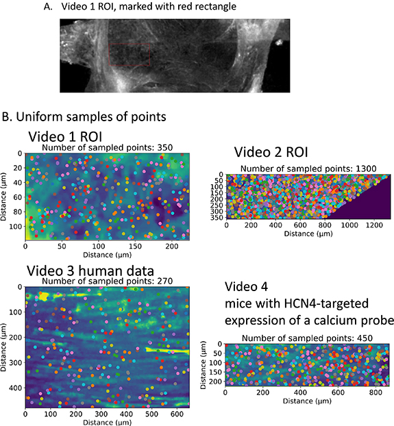
Figure 1. (A) Choice of ROI from calcium imaging data of the SAN; (B) choice of a uniform random sample from videos 1–4.
Download figure:
Standard image High-resolution imageIn this paper, we study several data sets. As the videos are quite short, i.e. the number of time frames is much smaller than the number of pixels, and for computational efficiency, we must choose only a subset of the pixels, with each pixel corresponding to a time series. To avoid subjectivity, we do not identify cells in the SAN. To extract a maximal amount of information, we number of time series we choose is approximately equal and a little smaller than the number of frames. To understand spatial properties of the calcium signals, we need to access the relationship between distance between pixels and covariance of the corresponding time series. Thus, we follow [22] in sampling the pixels uniformly at random so as to have a range of various distances available (picture of sampled points for each video can be found in figure 1(B)). A grid sampling in this case would not be appropriate as pixels in a grid have a minimum distance. We let S be the sample size. For our analysis of signalling cell modules, we also compare our findings from the uniformly random sample with a grid sample.
We notice that a key assumption in the RMT predictions is that the random variables have mean 0 and variance 1. Thus, upon obtaining our sample of time series, we normalize and demean it as is standard in financial literature, see e.g. equation (2) in [15]. Let time series Vi
be a time series in our sample with the index i running from 1 to the sample size, where Vi
is a function of t with  the magnitude of the ith signal at time t. Then we define and work with vi
as follows
the magnitude of the ith signal at time t. Then we define and work with vi
as follows

This procedure yields time series vi with mean 0 and variance 1, and thus the features of covariances of these time series can be meaningfully compared to the RMT predictions. The covariances of normalized and demeaned time series are the same as the correlations of the original time series.
Arranging the column vectors vi in some arbitrary order to form the T × S matrix V we study the matrix

Upon examining the eigenvalues and eigenvectors of C we find that the largest eigenvalue deviates from the RMT predictions by a vast amount and the corresponding eigenvector is delocalized. We demonstrate that this corresponds to system response to a common stimulus, in this case the AP-induced calcium transient propagating almost instantly via CX43. As we are interested in local rather than global signals we want remove the system response. We thus define another matrix of study in the following way, similar to [22]. Letting  be the eigenvector corresponding to the largest eigenvalue
  with
with  referring to the components, we define
the projection of all the time signals in a particular pixels onto the top eigenvector. Then using linear regression on each time series vi we obtain

where ai
and bi
are coefficients of linear regression and  is the residual. The T × S residual matrix R given by
  forms the new matrix for analysis, where all the original information remains intact except the influence of the top eigenvector is removed. Thus let

Lastly, in all our results we compare the properties of the data set with a control. As control we take the same matrix V and take a random permutation of the entries. We call this control matrix  , and define

This procedure destroys all correlations within the data, while keeping the properties of the individual random variables intact. Comparing spectral properties of C to ones obtained from  allows us to rule out the possibility that any anomalies are due to properties of the distribution of individual entries, such as heavy tails.
3. Results
3.1. Eigenvalues and eigenvectors
3.1.1. Eigenvalue distributions
Looking at the histograms of eigenvalues (figure 2), we see perfect agreement of our control with the RMT predictions with eigenvalues located in the predicted interval ![$[\lambda_-, \lambda_+]$](https://content.cld.iop.org/journals/2632-072X/4/1/015003/revision3/jpcomplexacadc8ieqn24.gif) . The histogram of the eigenvalues of C is also in agreement, but with a significant number of eigenvalues (
. The histogram of the eigenvalues of C is also in agreement, but with a significant number of eigenvalues ( 3%–6%) above
 ![$[\lambda_-, \lambda_+]$](https://content.cld.iop.org/journals/2632-072X/4/1/015003/revision3/jpcomplexacadc8ieqn26.gif) . We run basic checks to ensure that these properties do not depend overly much on the random sample of pixels that we have chosen. Basic properties of the eigenvalues and eigenvectors in 500 randomly chosen samples for videos 1 and 4 are shown in see figure 2(B). The box-and-whisker plot in figure 2(B) shows the distribution of the top eigenvalue which is proportionately close to the mean. The histogram in figure 2(B) shows that the number of eigenvalues outside the random matrix prediction range
. We run basic checks to ensure that these properties do not depend overly much on the random sample of pixels that we have chosen. Basic properties of the eigenvalues and eigenvectors in 500 randomly chosen samples for videos 1 and 4 are shown in see figure 2(B). The box-and-whisker plot in figure 2(B) shows the distribution of the top eigenvalue which is proportionately close to the mean. The histogram in figure 2(B) shows that the number of eigenvalues outside the random matrix prediction range ![$[\lambda_-, \lambda_+]$](https://content.cld.iop.org/journals/2632-072X/4/1/015003/revision3/jpcomplexacadc8ieqn27.gif) is also reasonably stable.
is also reasonably stable.
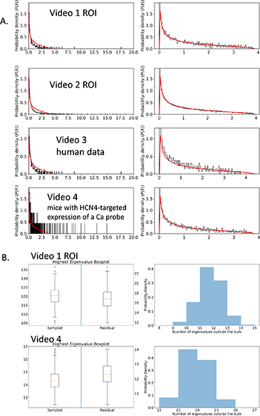
Figure 2. (A) Eigenvalues distributions of the correlation matrix for videos 1–4. Left column are eigenvalues of C, right is of  ; (B) stability analysis for various eigenvalue properties with 500 different random samples chosen for videos 1 and 4. On the left is a box plot for the top eigenvalue and on the right is for the number of eigenvalues outside of
 ![$[\lambda_-, \lambda_+]$](https://content.cld.iop.org/journals/2632-072X/4/1/015003/revision3/jpcomplexacadc8ieqn23.gif) for C.
for C.
Download figure:
Standard image High-resolution image3.1.2. IPR and eigenvector localization
Next we examine the IPRs (figure 3). In all the diagrams we see that the control IPRs (in orange) are low, and thus the eigenvectors are delocalized and follow the RMT predictions. The IPRs for the data are higher than those of control for eigenvalues larger than  except at
  . The higher localization at high eigenvalues indicates high correlations of particular pixels. Lastly, we see that the eigenvector associated to the highest eigenvalue is fully delocalized. This indicates a common response of the cell system to a common stimulus, in this case the AP-induced calcium transient.
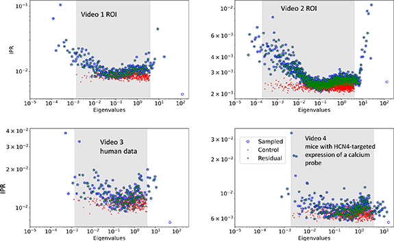
Figure 3. The IPR for videos 1–4, calculated separately for the control, sampled, and residual data. The x axis and y axis are log scaled. IPR values are on the y axis, and eigenvalues are on the x axis. The areas of the graph that are shaded in grey is interval predicted by RMT.
Download figure:
Standard image High-resolution imageAnalogously to [15], we identify the locations where the 2nd, 3rd, and 4th principal components are localized. In the study of cross correlations for financial returns, the places of principal component localization corresponded to various industries: such as companies with high market capitalization, semiconductors-computers, gold, Latin-American firms, etc. In our case, these will correspond to cell signalling modules. Since the eigenvectors are orthogonal and localized, these modules will be non-intersecting. In figure 4, we see the eigenvector components plotted in an arbitrary order, with a 2 standard deviation threshold. The components which exceed the threshold are places of eigenvector localization and when mapped back to the videos will signify signalling modules. We identify them with different colours in video 1, video 2, video 3, and video 4. Since we have taken a random sample of pixels, we map back five different samples to make sure that these identified signalling modules are not an artefact of a particular random sample. We see that the resulting modules are quite close (video 5); they are also quite close to those identified by a grid sample, see video 6. As the 2 standard deviation threshold is chosen arbitrarily, we verify that varying the threshold does not impact the identification of the signalling modules (see supplemental figure).

Figure 4. (A) Identification of signalling modules in video 1 i.e. places of localization of the eigenvectors corresponding to 2nd, 3rd and 4th highest eigenvalues; (B) average time series from the signalling modules for videos 1–4.
Download figure:
Standard image High-resolution imageWe then proceed to investigate the time series associated to the signalling modules. We average over the number of points, to obtain commensurate time series. The time series for video 1 turns out most remarkable of all. The localization of the top eigenvector identifies a signalling module that predicts the AP-induced calcium transient in every beat (in blue). Aside from this remarkable result, the average time series corresponding to other high eigenvalue eigenvectors as well as time series in the other videos demonstrate signals which are heterogeneous in amplitude and frequency, as established in [4], i.e. can vary from beat to beat or not be synchronized with the heartbeats at all.
3.2. Common response
The IPRs corresponding to the top eigenvector are low, indicating that the signal occurs in all the spatial pixels and corresponding to a common response. This is a global signal. For further analysis, in order to study local calcium signals, we remove the part corresponding to the common response. To do this we use the matrix  defined in equation (8). To verify that the top eigenvector indeed corresponds to common response, we study the correlation coefficient of a least squares regression between
  as defined in equation (6) and the time series representing the total signal mass at each time point
  . We obtain very high correlation coefficients for video 1 ROI (0.9975), video 2 ROI (0.9896), and video 3 (0.9686), and somewhat lower for video 4 (0.7147). On the other hand, taking the correlation coefficients between
  and similar projections onto the eigenvectors corresponding to the eigenvalues in the bulk we obtain a distribution with mean 0 and very low standard deviation for all videos: video 1 ROI (standard deviation 0.0019), video 2 ROI (standard deviation 0.0016), video 3 (standard deviation 0.0044), and video 4 ROI (standard deviation 0.0072). Thus the top eigenvector indeed correlates very strongly with the total signal mass and indicates common response, while the eigenvectors that are in line with RMT predictions do not correlate with total signal mass at all and indicate noise. The correlation for the similar projections onto the eigenvectors corresponding to the 2nd eigenvalues are small but much bigger than those for the bulk: for example for video 1 ROI, the correlation with the 2nd component is 0.034. For video 4, on the other hand, it is much higher than for video 1 ROI but still lower than with the principal component at 0.36.
As a control, we study the IPRs in figure 8. The blue circle and the red circle indicate the original signal and the time incremented signal while the blue dot and the red dot indicate the IPRs from the residual matrices. We notice that all the dots are exactly in the middle of their respective circles, except for the eigenvector that was removed, namely eigenvector corresponding to an eigenvalue above  with a low IPR. Thus this procedure of removing the common response is effective, and does not introduce any other effects.
3.3. Correlation coefficient structure and spatial correlations
We study the distribution of non-diagonal covariance coefficients. In figure 5, we plot in orange the control covariance coefficients, and observe that they are close to the theoretically predicted Gaussian. Compared to the orange control, the blue plot with the original data is heavily skewed to the right, indicating the presence of correlations. The residual correlation coefficients in green are far closer to the control, reflecting the removed global correlations in videos 1–3. Yet, they are still far from the Gaussian control, and skewed to the right, showing local correlations. To check that this is not a particular coincidence of our random sample we study 500 different samples from video 1 ROI and video 4 and construct histograms of the square error deviation (SED) from the control (figure 5(B)). In video 1, the SED is large for C and much smaller (an order of magnitude) for  . This demonstrates that the removed top eigenvector indeed corresponds to global response. In video 4, however, this effect is less pronounced and the SED from control is commensurate for C and
  . We speculate in discussion that this is due to a slower signal propagation, yielding stronger time correlations and weaker space correlations.
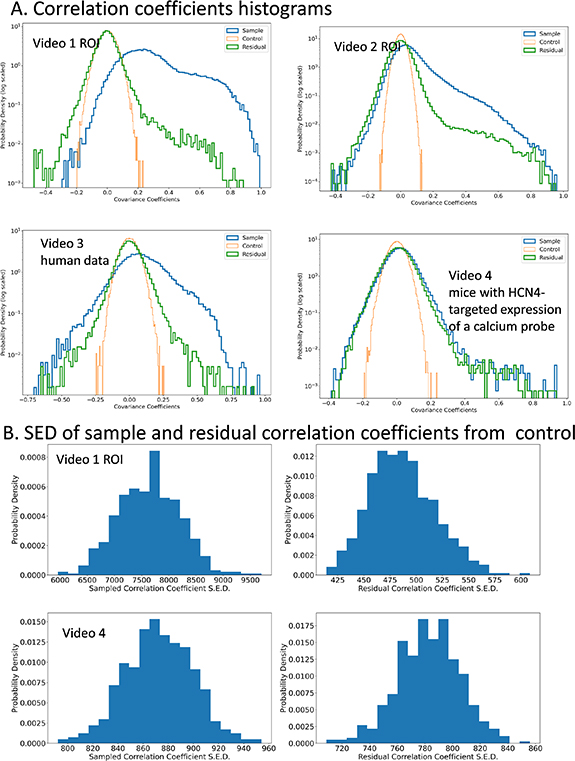
Figure 5. (A) Histograms of various covariance coefficients for videos 1–4. Blue is from the original normalized data sample. Green is from residuals, representing common response to stimulus removed. Orange is control from all entries of the original data randomized; (B) total square error of deviation from control (obtained from  ) of all the histograms from (A) in videos 1 and 4.
Download figure:
Standard image High-resolution imageLastly, another important result we can obtain using information on correlation coefficients is the presence of correlations at distances which are higher than cell size. The SAN node cell is known to be roughly spindle shaped at 5–10 µm in diameter and 20–30 µm in length [3]. We sort the correlation coefficients in the upper triangle of  according to distance between the pixels and make a separate normalized histogram for pixels with distances 0–20 µm (blue), 20–40 µm (orange), 40–60 µm (green), 60–80 µm (red), etc and we can use far-apart points as control. We see strong deviations from the control in all the distance histograms for video 1, 2, and 3 (figures 6(A)–(C)), particularly in the right tails of the distribution. In figure 6(D), we plot the integral of the tail, equivalent to the proportion of correlation coefficients larger than 0.3 for videos 1, 3, and 4. In videos 1 and 3, this proportion can be seen to be very high at distances 0–20 µm and 20–40 µm. However, the proportions of higher correlations present at distances higher than 40–60 µm and 60–80 µm, visible particularly in the tails plot, indicate intercellular correlations. This proportion is nearly 0 at distances over 80 µm, which can be used as a control. In video 4, however, the correlations at intercellular distances appear weaker, see section 4.

Figure 6. Histograms of covariance coefficients sorted by distance for videos 1, 2, and 4, blue for 0 to 20 µm, orange for 20–40 µm, green for 40–60 µm, red for 60–80 µm, grey for control. Also the integrals of the histogram tails for videos 1, 3, and 4.
Download figure:
Standard image High-resolution imageOne more check on spatial vs time correlations reveals that space correlations are much more significant than time correlations (figure 7). The histogram of space correlations is as before constructed from the upper triangle of C. To access the time correlations we demean and renormalize the rows instead of the columns, and then construct a T × T matrix by multiplying the other way. We see that the pink histogram for time correlations is closer to a Gaussian. This means that the time correlations are not too high and our RMT approach is valid. However, as noted before in video 4 there is a stronger presence of time correlations.

Figure 7. PDF histograms of space correlations (blue) and time correlations (pink) for videos 1–4.
Download figure:
Standard image High-resolution image
Figure 8. (A) Distribution of distances between nearest unfolded eigenvalues from videos 1–4, blue for unfolded data, pink for shuffled control, red for RMT prediction; (B) the number variance for videos 1–4, with red line for Poisson process, blue line for RMT predictions, and circles for shuffled control.
Download figure:
Standard image High-resolution image
4. Discussion
In this paper, we have investigated the structure of correlation coefficients between calcium time series at different locations within the SAN using experimental data imaged from intact tissue. The aim is to use RMT to understand properties of calcium signals in SAN and to glean fundamental insights into the workings of SAN. The fundamental question with regard to the SAN is how each AP-induced calcium transient, which corresponds to a single heartbeat, is initiated. It has been shown in [4] that signals at various locations of the SAN are remarkably heterogeneous. Here we take a step toward a mechanistic understanding of the system by demonstrating that the signalling cells interact, thus forming a complex system with heart rate as an emergent phenomenon. How exactly the heart rate emerges from the heterogenous signalling units remains unclear, with both the exact biophysical means of cell interaction and the mathematical mechanism of heart rate emergence requiring further research.
Our analysis is based on RMT. We separated the eigenvalues of the signal correlation matrix, and into the parts that are due entirely to noise (those consistent with RMT predictions), those which are due to common response to AP-induced calcium transient (which we can remove for further analysis, e.g. so as to understand the distance-dependence of correlations), and those due to local spatial correlations. We then checked where the eigenvectors are localized indicating points in space where the calcium signal changes jointly, thus identifying signalling cell modules. In one of our cases, the eigenvector localization corresponding to second highest eigenvalue (recall that the highest corresponds to global response and is not relevant for local calcium signalling analysis) identified a signalling module that initiated the AP-induced calcium transient. This 'precursor' module could be a pacemaker module or a signal processing module. It is possible that although we tried to avoid CX43 cells in the ROI, this module is an extension of the 'railroad track' CX43 network that carries the excitation. In this case, it is where the central zone first passes the signal to the 'railroad track' zone. Further studies could be performed to ascertain how frequently such a 'precursor' module is so clearly identified, how it works, and how it is best interpreted.
In our analysis of correlation, we see that video 4, namely the calcium imaging video from the central area of SAN recorded in preparation from a genetically modified mouse pCAGGS-GCaMP8 with HCN4-targeted expression of Ca2+ probe, has different properties from the other videos. This demonstrates the value of our approach, as these subtle differences in the calcium signals could not be picked up by inspection. We see that the spatial correlations at intercellular distances are smaller than in other videos. We also see that the global response is much less pronounced, as the top eigenvalue is commensurate with the second largest eigenvalue, the top eigenvector is less delocalized, and the correlation coefficient between the signal average and the projection of signals onto the top eigenvector is smaller. These effects could be stemming from differences in the part of the central zone chosen for analysis or from the experimental conditions. We also see that the time correlations in video 4 are not small compared to the space correlations (figure 8), which can impact the assumptions of our analysis and could indicate slower signal propagation.
As shown on other systems [16, 22], number variance is a very sensitive parameter. Further studies of the number variance could reveal systematic changes based on various experimental conditions. The number variance could be a characterizing feature of the system and therefore could in the future be useful for diagnostics. However, in using the number variance, we must be cautious of finite size effects, as the number variance for the longest video (video 2) is the closest to the RMT prediction.
Some of the study limitations are as follows. The analysis was done on only four videos. A future study might conduct this analysis on a large number of videos, and compare the results. It would be interesting to determine how the identified signalling modules of cells interact and create the AP transient. Another limitation is the presence of time correlations which we neglect. We have demonstrated qualitatively that they are small, however, a means of quantitatively establishing how small and how such correlations impact the RMT predictions could be developed in the future. RMT for matrices with dependence in the columns is currently available, cf e.g. [1], and predicts a different distribution of eigenvalues if the dependence is strong enough. This theory can be further developed should there be important statistical applications. Our aim of objective mathematical analysis is only partially achieved, as the identification of ROI was still done by visual inspection. This could be improved, perhaps with machine learning or direct thresholding to identify the central SAN in immunolabelled images. At this point, for example, it is not clear that the module seen to initiate the signal in video 1 carries no CX43. Lastly, the histograms for correlation coefficients sorted by distance in figure 6 have a dependence on the video length, which is why we give the analysis for the three videos whose lengths are commensurate. If there were no time dependence, it is clear that by the central limit theorem the correlation coefficients would scale by  . However, since there is time dependence, more sophisticated models of time series must be found or developed to understand the correct scaling. In particular, the coefficients for the longest video (video 2) exhibit the same pattern as a function of distance, but are smaller by about a factor of 50 in absolute magnitude. Another limitation to note is that our methods do not offer causal relationship to our results. We do not analyse what causes the pixels of the identified signalling modules to be working as a unit: it may be ryanodine receptor clusterization, some peculiarity of the subcellular matrix that allows for easy calcium diffusion, or even they might be operating as unit by chance. Additionally, while we can identify signals which are local and those which are global via a study of IPRs we cannot infer that the local signals are not caused by the AP.
Our methodology is very robust, and can be applied to further data sets to identify signalling modules. Some possibilities for future studies include further studies of the SAN under various experimental conditions. Further methodological development and direction of future research could be to understand the speed of calcium propagation by studying the delay that maximises correlation of a pairs of time series.
While SAN numerical modelling is a long-standing area of research, the classic models of SAN such as [23] are not agent-based and thus cannot assess local activity. Agent-based models of the SAN have only recently been developed with the aim of understanding how local cell heterogeneity impacts pacemaking [5, 11]. However, the two recent models do not include local calcium signalling, instead relying on electrophysiological mechanisms and common-pool calcium for cellular pacemaking. A natural and crucial next step in a mechanistic understanding of the SAN would be to develop an agent-based model using in-silico cells that feature local calcium releases such as in [12]. This approach could explain the nature of the signalling modules we identify here, which would yield key insight into what factors crucially contribute to heartbeat initiation. In particular, we expect the signalling modules we find are due to some heterogeneity in the cellular or subcellular structures. This could be modelled with random parameters in a mechanistic model. Potential parameters that can be randomised include locations or sizes of RyR clusters inside the cells, speed of sarco/endoplasmic reticulumCa2+-ATPase pumping, cell size and geometry, L-type calcium channel isoforms, RyR phosphorylation levels, and many other possibilities. The RMT-based methods of the present paper could be used to understand the generated model data, offering a fair comparison with experiment.
5. Conclusions
This paper is a first application of RMT based methods to calcium imaging in the SAN. We borrow and adapt powerful methods that have been used to study correlations various data sets such as finance, EEGs, and calcium imaging in β-collective cells. We are able to separate out eigenvalues of the correlation matrix arising from noise, those arising from local correlations, and those indicating a global response. We can furthermore identify signalling modules based on localization properties of eigenvectors and study distance dependence of correlations. This work opens great possibilities for future studies, such as analysis of further data from experiment or mechanistic numerical models to understand how various interventions might impact the correlation structures of calcium signals. For example, an intervention might change the signalling landscape and the signalling modules might shift. Furthermore, the number variance might be developed into a diagnostic tool, as it is known to change under various experimental conditions.
Acknowledgment
The authors gratefully acknowledge the support of the Royal Society University Research Fellowship UF160569. We are also grateful to Prof. Dean Korošak for useful discussions and for sharing the Python code from [22].
Data availability statement
No new data were created or analysed in this study.
Conflict of interest
The authors declare that the research was conducted in the absence of any commercial or financial relationships that could be construed as a potential conflict of interest.
Appendix.: Wigner surmise
Here we demonstrate that the eigenvalue spacing for the eigenvalues predicted by RMT follows the Wigner surmise, which is a universal distribution for eigenvalue spacing that arises in theoretical mathematics, as well as in numerous real-world examples including spacings of energy levels in heavy atoms, bus timings in Cuernavaca, Mexico [10], correlations in EEG data [16] as well as the two systems that inspired this work: financial markets and β-collectives. The fact that the eigenvalue distances follow the Wigner surmise confirms that the RMT-predicted eigenvalues correspond to system noise, and this noise has universal properties i.e. it is not special or unusual. We also examine the number variance and find that it is far more sensitive to experimental conditions, in line with prior work on human EEGs [16] and pancreatic β-cells [22].
The distances between nearest eigenvalues are also well-understood. They were studied by Wigner in a random matrix model where eigenvalues corresponded to energy levels in a heavy nucleus and the RMT prediction described the repulsion between them (i.e. two quantized energy levels cannot be too close to each other). The probability density P for the distances between nearest eigenvalues is universal for many ensembles, once the eigenvalue density is accounted for. This normalization for the eigenvalue density is called spectral unfolding. The density P is then given by the 'Wigner surmise' equation see e.g. section 1.5 of [14]

To probe the finer structure of eigenvalue correlations, one introduces the number variance  . Letting ξ be an unfolded eigenvalue and
 ![$\mathcal{N}([a, b])$](https://content.cld.iop.org/journals/2632-072X/4/1/015003/revision3/jpcomplexacadc8ieqn41.gif) be the number of eigenvalues in the interval
be the number of eigenvalues in the interval ![$[a,b]$](https://content.cld.iop.org/journals/2632-072X/4/1/015003/revision3/jpcomplexacadc8ieqn42.gif) , the number variance is given by
, the number variance is given by

where  denotes the ensemble average. Here the average is taken over unfolded eigenvalues ξi
in the middle of the eigenvalue distribution. The RMT prediction for the number variance is
denotes the ensemble average. Here the average is taken over unfolded eigenvalues ξi
in the middle of the eigenvalue distribution. The RMT prediction for the number variance is

see e.g. section 16.1 of [14].
Here we work with a time-incremented time series. This is analogous to working with returns rather than prices in financial mathematics, which decreases the impact of correlations within a time series on the analysis. The time incremented eigenvalues closely follow the Marchenko–Pastur law and thus are easier to unfold. We define the series  by
by  . Then we work with
  , where
  is
is  demeaned and normalized using equation (4). It is important that the time incrementing happens first, and the demeaning and normalization second, so that the resulting variables are of mean 0 and variance 1.
We unfold the spectrum by using the Marchenko–Pastur law (2) as our limiting density, and we implement a classic procedure whereby we map each eigenvalue Ej
to a new variable  . In this analysis, we neglect the eigenvalues
  and
and  . The resulting histogram of distances between nearest eigenvalues, avoiding largest 20% and smallest 20% of eigenvalues, is shown in figure 8 in blue. We perform the same procedure for the eigenvalues of the control matrix
  , and it is plotted in figure 3(A) in pink. We observe a close match to the Wigner surmise distribution in all analysed videos, with a somewhat better match for the control case.
We then proceed to compute the number variance  , which captures higher order correlations between the eigenvalues (figure 8(B)). We use the same unfolding procedure, and only average over the middle 60% of eigenvalues to avoid edge effects. We see significant deviations from both the RMT prediction as well as from the Poisson process, thus the eigenvalues are correlated but not as much as eigenvalues of random matrices. This is in line with prior research on EEGs and β-cell collectives [16, 22].
Supplementary data (19. MB PPTX) Identification of signalling modules using different thresholds. The threshold value does not significantly impact the results.
Supplementary data (4.4 MB PPTX) Analysis for a smaller sample of time series for Video 1
Supplementary data (37. MB PPTX) Videos 1 - 4 with identified signalling modules