
Abstract
In this work we analyze structural and spectral properties of a model of directed random geometric graphs: given n vertices uniformly and independently distributed on the unit square, a directed edge is set between two vertices if their distance is smaller than the connection radius  , which is randomly drawn from a Pareto distribution. This Pareto distribution is characterized by the power-law decay α and the lower bound of its support
  ; thus the graphs depend on three parameters
  . By increasing
  , for fixed
  , the model transits from isolated vertices (
 ) to complete graphs (
 ). We first propose a phenomenological expression for the average degree
  which works well for α > 3, when k is a self-averaging quantity. Then we numerically demonstrate that
 ![$\langle V_x(G) \rangle \approx n[1-\exp(-\langle k\rangle]$](https://content.cld.iop.org/journals/2632-072X/4/1/015002/revision2/jpcomplexacace1ieqn9.gif) , for all α, where
, for all α, where  is the number of nonisolated vertices of G. Finally, we explore the spectral properties of
  by the use of adjacency matrices represented by diluted random matrix ensembles; a non-Hermitian and a Hermitian one. We find that
  is a good scaling parameter of spectral and eigenvector properties of G mainly for large α.
Export citation and abstract BibTeX RIS

Original content from this work may be used under the terms of the Creative Commons Attribution 4.0 license. Any further distribution of this work must maintain attribution to the author(s) and the title of the work, journal citation and DOI.
1. Introduction
Graphs and networks are nowadays well accepted tools to model complex systems. Moreover, if the system under study is embedded in a geometric space (like road networks, power networks or networks of wireless communication devices) the best suited representation belongs to the so-called spatial networks [1]. In this respect, probably the most studied model of spatial networks is the random geometric graph (RGG) model [2, 3] introduced by Gilbert in 1959 [4].
In Gilbert's original version a RGG consists of n vertices uniformly and independently distributed on the infinite plane, where two vertices u and v are connected by an edge if their Euclidean distance is less or equal than the connection radius  [4, 5]. Moreover, since Gilbert's pioneering work, several variants of RGGs have been proposed to account for the properties of realistic complex systems: Commonly, RGGs are considered inside bounded domains such as the unit square [2, 6], the unit circle, see e.g. [7], or d-dimensional cubes and spheres [8]. Also, recently, RGGs over more intricate bounding domains (i.e. elongated rectangles [9–11] or annuli [12, 13]) have been studied. RGGs with non-uniform vertex distributions have been explored too [14–16]; while quasirandom vertex distributions have also been considered in [17]. Additionally, motivated by wireless ad hoc networks, there is a generalization of RGGs, known as soft RGGs [18], where the connection between vertices obeys a probabilistic function; see also [12, 19].
It is interesting though that even when most of the real-world spatial networks that could be modeled by RGGs (i.e. transportation networks like cargo ship networks, infrastructure networks like power networks or road networks, communication networks, etc) and the processes associated to them (i.e. disease spreading, urban sprawl, commuter behavior, etc) are intrinsically directed, models of directed RGGs have been scarcely studied. For exceptions see [20, 21] where models of directed RGGs have been used to study wireless networks and word association networks, respectively. Therefore, to contribute to fill this gap, in this work we numerically explore structural and spectral properties of a model of directed RGGs.
2. Random graph model
In this work, we consider the following model of directed RGGs (dRGGs): given n vertices uniformly and independently distributed on the unit square we randomly assign the connection radius  to the vertex u, where
  is taken from a Pareto distribution,

Here, α > 0 is the power-law decay of the Pareto distribution, ![$\ell_0\in(0,\sqrt{2}]$](https://content.cld.iop.org/journals/2632-072X/4/1/015002/revision2/jpcomplexacace1ieqn16.gif) is the lower bound of the support of the distribution, and
is the lower bound of the support of the distribution, and

is a normalization factor such that  . In figure 1 we show some examples of probability distribution functions
  for different combinations of α and
  . Then, if the vertex v lies within the disc of radius
  , centered at u, there is a directed edge from u to v,
  . Note that since
  , the existence of
  does not imply
  , so the graph is directed. Therefore, this model of dRGGs depends on three parameters:
  .
.

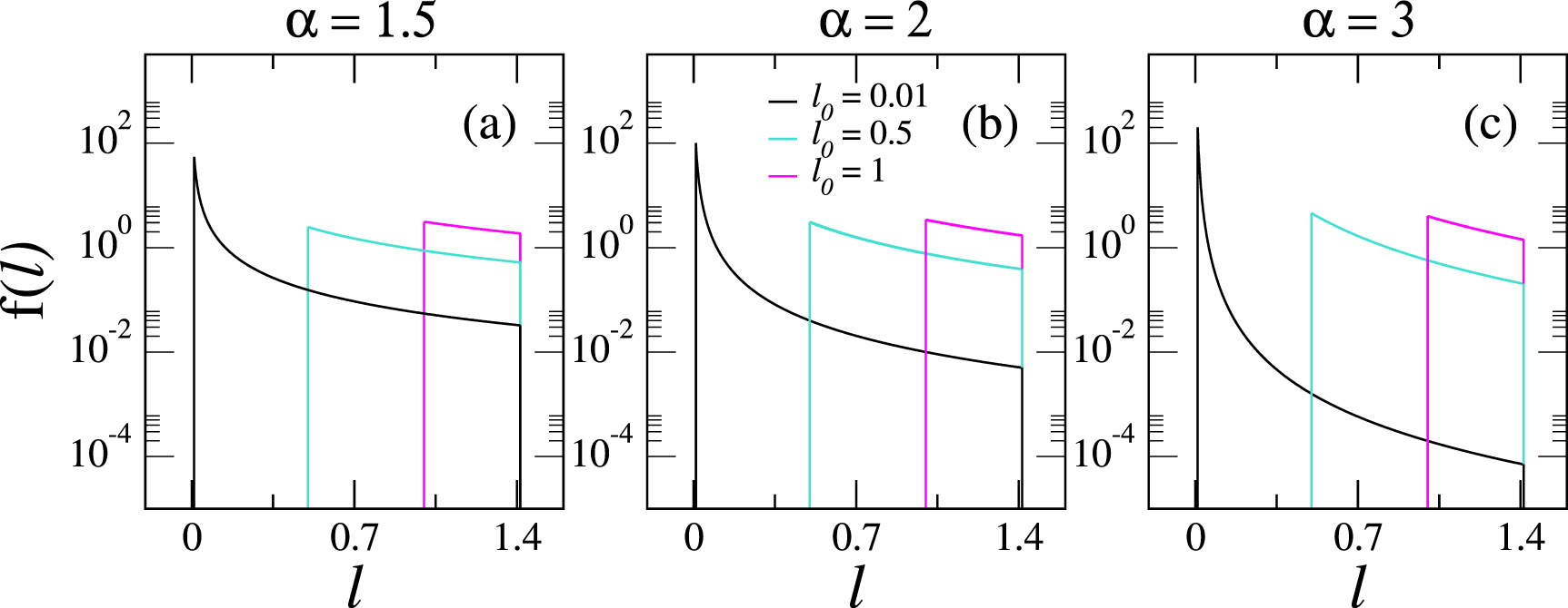
Figure 1. Probability distribution functions  , see equation (1), for (a) α = 1.5, (b) α = 2, and (c) α = 3. Each panel displays
  with
with  , 0.5, and 1.
Download figure:
Standard image High-resolution imageIt is fair to mention that the random graph model  we study here is inspired by that introduced in [21], with three important differences: (a) we consider vertices distributed on the unit square instead of on a two dimensional torus. Indeed, in [21] the graph model is more general since vertices are considered on a d-dimensional torus. (b) We consider α > 0 instead of
  , so here we can approach the case of a flat
  when α → 0. (c) We consider
  as a free parameter in the range
 ![$(0,\sqrt{2}]$](https://content.cld.iop.org/journals/2632-072X/4/1/015002/revision2/jpcomplexacace1ieqn33.gif) , while in [21] it is set to
, while in [21] it is set to  (for the two dimensional torus), such that the resulting graph is almost surely connected. So here we can explore the limit
  producing graphs with mostly isolated vertices.
Thus, the model of dRGGs defined above shows a transition by increasing  , for fixed
  , from isolated vertices when
  to complete graphs for
  . However, large values of α also enhance the existence of isolated vertices; see for example the black distribution in figure 1(c) which is strongly peaked at
  .
.
In section 4 we explore structural and spectral properties of dRGGs. In particular, we analyze the spectral properties of the model by the use of a recently introduced approach under which the adjacency matrices of random graphs are represented by diluted random matrix theory (RMT) ensembles 1 . In this respect, Erdös-Rényi graphs and RGGs have been represented by diluted versions of the Gaussian orthogonal ensemble (GOE) [11, 24], multilayer and multiplex networks have been studied through diluted-banded random matrix ensembles [25], while bipartite and mutualistic networks were analyzed by the use of block-diluted random matrix ensembles [26]. Here, within the same approach, we use two adjacency matrix representations that we define as follows.
2.1. Randomly weighted non-Hermitian adjacency matrix
We define the elements of the non-Hermitian adjacency matrix  of the dRGGs as

where εuv
are independent random variables drawn from a normal distribution with zero mean and unit variance;  since
since  is directed. According to this definition, diagonal random matrices (known in RMT as the Poisson ensemble (PE) [27]) are obtained for
  , when the graphs consist mostly of disconnected vertices; whereas the real Ginibre ensemble (RGE) (i.e. full real and non-symmetric random matrices [28]) is recovered for
  , when the graphs are complete. Therefore, we expect to observe a transition from the PE to the RGE for increasing
  . Thus, the ensemble defined by
  corresponds to a diluted RGE.
2.2. Randomly weighted Hermitian adjacency matrix
Additionally, given the standard binary adjacency matrix B extracted from the directed graph  , we consider the following Hermitian adjacency matrix
  :
:

Again, εuv
are independent random variables taken from a normal distribution with zero mean and variance one. It is clear that ![$[A_H]_{vu} = [A_H]_{uv}^*$](https://content.cld.iop.org/journals/2632-072X/4/1/015002/revision2/jpcomplexacace1ieqn50.gif) by construction. In fact,
by construction. In fact,  , with the name of magnetic adjacency matrix, was already used in [29] to represent randomly-weighted Erdös-Rényi directed graphs; while the unweighted version of
  was introduced in [30]. The main advantage of
  over
over  is that the former has a real spectrum, thus some spectral measures from RMT can be computed easier.
Therefore, the magnetic random matrix ensemble (MRME) defined by  transits for increasing
  from the PE, when
  , to the GOE (i.e. full real and symmetric random matrices [27]), when
  . However, note that the MRME can not be considered as a diluted GOE since for any
  ,
,  is a complex Hermitian matrix.
3. Characterization measures
3.1. Structural measures
In addition to the standard quantities used to characterize the structure of random graphs and networks, such as the statistical properties of the vertex degree k and the average number of nonisolated vertices Vx , here we also use topological indices.
Given a simple graph  with V(G) and E(G) the vertex set and edge set, respectively, the Randić connectivity index is defined as [31]

while the Harmonic index is given by [32]

Here uv denotes the edge connecting vertices u and v and ku the degree of vertex u:

where  and
and  are the in-degree and out-degree of vertex u.
From definitions (5) and (6), when  (i.e. when the model of dRGGs produces mostly isolated vertices),
  and
and  ; while for
  (i.e. when the graph model produces complete graphs),
  and
and  . That is, when applying R(G) and H(G) to ensembles of random graphs characterized by the parameter set
  , we expect to observe a transition from
  and
and  to
to  and
and  when increasing
  from
from  to
to  .
.
We stress that the random weights we impose to the adjacency matrices  and
and  , as defined respectively in equations (3) and (4), do not play any role in the computation of the degree-based topological indices.
In fact, within a statistical approach to random graphs, it has been recently shown that the average values of R(G) and H(G), normalized to the order of the graph n, scale with the average degree  ; see e.g. [33–35]. That is,
  and
and  are functions of
  only. Moreover, it was also found that
  and
and  are highly correlated with the Shannon entropy of the eigenvectors of the adjacency matrix of RGGs [36]. This is a notable result because it puts forward the application of degree-based topological indices beyond mathematical chemistry (it is relevant to add that random graphs have also been studied by means of eigenvalue-based topological indices such as the Estrada index, the Laplacian Estrada index, and Rodriguez-Velazquez indices, see e.g. [37, 38]). Therefore, the study of R(G) and H(G) on dRGGs seems to be pertinent.
3.2. Spectral measures
We use standard RMT measures to characterize spectral and eigenvector properties of the non-Hermitian  and Hermitian
  adjacency matrices defined, respectively, in equations (3) and (4).
Regarding spectral properties, for  which has complex spectra, we use the ratio between nearest- and next-to-nearest-neighbor spacings
  , with the ith ratio defined as [39]

where  and
and  are, respectively, the nearest and the next-to-nearest neighbors of λi
in
are, respectively, the nearest and the next-to-nearest neighbors of λi
in  . While, given the real and ordered spectrum of
  ,
,  , we compute the ratio between consecutive level spacings
  , where the ith ratio is given by [40]

Note that  can also be computed for real spectra, so it works for both
  and
and  .
.
Regarding eigenvector properties, given the normalized eigenvectors  (i.e.
(i.e.  ) of
) of  or
or  , we compute the inverse participation ratios [41]

and the Shannon entropies [42]

Both  and S measure the extension of eigenvectors on a given basis, so in the case of random graphs they can be used to prove percolation transitions; see e.g. [24, 36].
From definitions (8)–(11), when  (i.e. when
  and
and  are mostly diagonal),
  ,
,  ,
,  , and
, and  ; while for
  (i.e. when
  and
and  are full random matrices), all spectral and eigenvector measures are expected to acquire their corresponding full random matrix values.
4. Analysis of structural and spectral properties
4.1. Structural properties
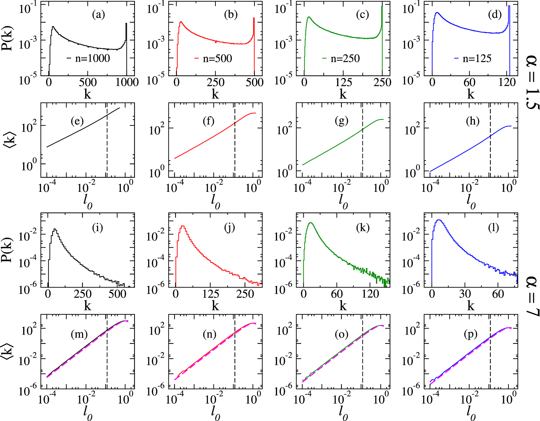
We start by exploring some statistical properties of the vertex degree k of the model of dRGGs. In figure 2 we present examples of degree distributions P(k) for different graph sizes n (different columns correspond to different values of n) and two values of α: α = 1.5, panels (a–d), and α = 7, panels (i–l). We note that, for fixed α, the support of P(k) grows with n while keeping the shape; indeed the shape of P(k) evolves with α. Specifically, while for small α, P(k) develops a two-peak structure (one broad peak for k → 1 and one sharp peak at  , see e.g. panels (a–d) for α = 1.5), P(k) is unimodal for large α (see e.g. panels (i–l) for α = 7). Moreover, we observe a smooth transition in the shape of P(k) from the two-peak structure to the unimodal form for increasing α; see for example figures 3(a)–(e), where we show P(k) for several values of α. Notice, though, that in figures 3(a)–(e) we are plotting distributions of the normalized degree
 , where
  is the variance of k, to show that the shape of
  depends on α only.

Figure 2. (a)–(d), (i)–(l) Degree distributions P(k), at  , and (e)–(h), (m)–(p) average degree
  as a function of
  for dRGGs. Each column corresponds to random graphs of different size n. Panels (a)–(h) and (i)–(p) correspond to α = 1.5 and α = 7, respectively. Vertical black-dashed lines in (e)–(h), (m)–(p) mark
  , the value of
  used to compute P(k) in (a)–(d), (i)–(l). Magenta dashed lines in (m)–(p) are equation (12). Both P(k) and
  were computed from
  random graphs.
Download figure:
Standard image High-resolution image
Figure 3. (a)–(e) Probability distribution function of the normalized degree  for dRGGs with
  . (f)–(j) Average degree
  (normalized to n − 1) as a function of
  . Magenta dashed lines in (f)–(j) are the best fittings of equation (13) to the data; the fitting constants are reported in table 1. (k)–(o) The variance of the degree
  (normalized to n2) and (p)–(t) the ratio
  as a function of
  . In all panels we report results for four different graph sizes n. Each column corresponds to a different value of the power-law decay α.
Download figure:
Standard image High-resolution imageAlso, in figure 2 we plot the average degree  as a function of
  for dRGGs characterized by α = 1.5, panels (e)–(h), and α = 7, panels (m)–(p). In particular, we noticed that the curves
  vs.
vs.  for α = 7 can be well described by the expression for
  , derived in [9], for standard RGGs when replacing
  by
by  :
:

see the magenta dashed lines in figures 2(m)–(p). This fact makes sense to us because, for large α,  is strongly peaked at
  so most radii get the value of
  . Moreover, taking into account that we are dealing with a distribution of radii
  , we found that

describes the average degree of dRGGs with α > 3 even better than equation (12). In equation (13), Ci
are fitting constants and  is the average connection radius that we computed directly from equation (1) as

where η is given in equation (2). An important consequence of equation (13) is that the ratio  does not depend on n, as it is verified in figures 3(f)–(j) for all values of α (not only for α > 3): there, in each panel, we present four curves for different graph sizes n that fall one on top of the other, as anticipated. Thus, in figures 3(f)–(j) we plot equation (13) (as magenta dashed lines) and see a very good correspondence with the numerical data for α > 3, while for smaller α we see good correspondence for large
  only. Notice form table 1 that the value of the fitting constant C1 is approximately equal to π for all α; therefore, the prediction for
  for standard RGGs from [9] with
  approximately coincides with equation (13) to the leading order.
Table 1. Values of the fitting constants Ci of equation (13) for different values of α. The fittings were performed on the data of figures 3(f)–(j).
| α = 1.5 | α = 2 | α = 3 | α = 4.5 | α = 7 | |
|---|---|---|---|---|---|
| C1 | 3.203 | 3.147 | 3.192 | 3.274 | 3.340 |
| C2 | 3.220 | 3.081 | 3.113 | 3.216 | 3.292 |
| C3 | 0.929 | 0.857 | 0.856 | 0.887 | 0.907 |
To complete the statistical inspection of k, in figures 3(k)–(o), we show that the variance of k grows with  , approaches a maximum, and then decreases to zero for
  ; where the maximum is higher the larger the value of α is. Also, in figures 3(p)–(t), we plot the ratio
  as a function of
  . It is interesting to note that for small α,
  remains constant for increasing graph size (that is, the curves in panels (p, q) fall one on top of the other for different n), meaning that k is not a self-averaging quantity. On the contrary, for large α and small
  , the ratio
  decreases with n (see the left part of the curves in panels (s, t)); so, under these conditions, k is a self-averaging quantity.
Now, we recall that increasing  from
from  to
to  drives the model of dRGGs from mostly isolated vertices to complete graphs. This transition, as a function of
  , could be well characterized by computing the average number of nonisolated vertices
  as well as the average values of the Randić and the Harmonic indices, see e.g. [36]. Certainly, we expect
  when
when  and
and  for
for  .
.
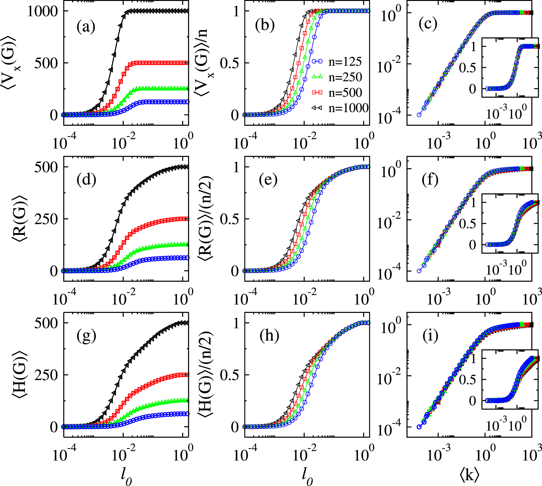
Then, in figures 4(a), (d) and (g) we present, respectively, the average number of nonisolated vertices  , the average Randić index
  , and the average Harmonic index
  as a function of
  of dRGGs characterized by α = 3. We show curves for four different graph sizes n in each panel. As can be clearly seen, the three quantities
  (where X represents Vx
, R or H) undergo a smooth transition (in log scale) from
(where X represents Vx
, R or H) undergo a smooth transition (in log scale) from  for small
  to the corresponding maxima
 ![$\mbox{max}[X(G)]$](https://content.cld.iop.org/journals/2632-072X/4/1/015002/revision2/jpcomplexacace1ieqn187.gif) at
at  . Moreover, the normalized curves
 ![$\langle X(G)\rangle/\mbox{max}[X(G)]$](https://content.cld.iop.org/journals/2632-072X/4/1/015002/revision2/jpcomplexacace1ieqn189.gif) vs.
vs.  have a very similar functional form but they are displaced to the left on the
  –axis for increasing n; see figures 4(b), (e) and (h). In fact it was shown, for standard RGGs [36] and also for non-uniform RGGs [14], that these three normalized quantities scale with
  ; that is, the curves
 ![$\langle X(G)\rangle/\mbox{max}[X(G)]$](https://content.cld.iop.org/journals/2632-072X/4/1/015002/revision2/jpcomplexacace1ieqn193.gif) vs.
vs.  fall one on top of the other for different graph sizes. Therefore, we validate this scaling for dRGGs in figures 4(c), (f) and (i) where we plot
  ,
,  and
and  vs.
vs.  in log–log scale (main panels) as well as in semilog scale (insets). While we observe a very good scaling for the average number of nonisolated vertices, the scaling of both the Randić and the Harmonic indices is good for
  only.
only.

Figure 4. (a) Average number of nonisolated vertices  , (d) average Randić index
  , and (g) average Harmonic index
  as a function of
  of dRGGs characterized by α = 3. In each panel we report results for graphs of four different sizes n. Normalized average indices
  ,
,  , and
, and  as a function of (b), (e), (h)
  and (c), (f), (i)
  . The insets in (c), (f), (i) show the same curves of the main panels but in semilog scale. All averages were computed from
  random graphs.
Download figure:
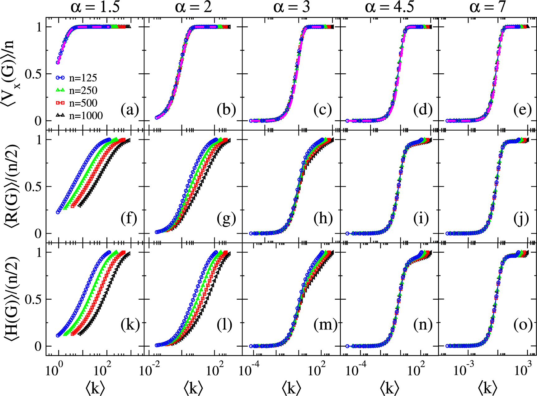
Standard image High-resolution imageFurthermore, in figure 5 we explore the scaling of ![$\langle X(G)\rangle/\mbox{max}[X(G)]$](https://content.cld.iop.org/journals/2632-072X/4/1/015002/revision2/jpcomplexacace1ieqn200.gif) with
with  for dRGGs characterized by values of α ranging from 1.5 to 7. We do confirm that
  shows a perfect scaling with
  for all the values of α examined in this work; see figures 5(a)–(e). In contrast, the scaling of
  and
and  with
with  is reasonably good for α > 3 only; indeed for α < 3 these two indices do not scale in any range of
  , see figures 5(f), (g), (k) and (l). We surmise that the lack of scaling of
  and
and  with
with  , for small α, may be related to the non self-averaging property of k for those values of α.

Figure 5. (a)–(e) Normalized average number of nonisolated vertices  , (f)–(j) normalized average Randić index
  , and (k)–(o) normalized average Harmonic index
  as a function of the average degree
  for dRGGs of four different sizes n. Magenta dashed lines in (a)–(e) are equation (16). Each column corresponds to a different value of the power-law decay α. All averages were computed from
  random graphs.
Download figure:
Standard image High-resolution imageWe also recall that an expression for  is known for standard RGGs [43]:

which was recently generalized for both RGGs and non-uniform RGGs as [14]

Then, given the perfect scaling of  with
with  (meaning that
  is a function of
  only), we test equation (16) on dRGGs by plotting it in figures 5(a)–(e); see the magenta dahsed lines. Indeed, we do confirm that equation (16) describes perfectly well our numerical data for all α. This is a remarkable result because it stresses the universality of equation (16) on RGGs models.
4.2. Spectral properties
We now explore some spectral properties of dRGGs. We perform exact numerical diagonalization to obtain the eigenvalues λi
and eigenvectors 
 of large ensembles of randomly-weighted adjacency matrices
  and
and  characterized by the parameter set
  .
.
In figures 6(a), (d) and (g) we present, respectively, the average ratio between consecutive eigenvalue spacings  , the average inverse participation ratio
  , and the average Shannon entropy
  as a function of
  for dRGGs characterized by α = 3. Note that here the dRGGs are represented by the diluted RGE; i.e. by the non-Hermitian adjacency matrices
  of equation (3). In each panel we report results for graphs of four different sizes n. As for the structural measures (see figures 4(a), (d) and (g) as a reference), the three spectral measures
  (where X represents
  ,
,  or S) undergo a smooth transition (in log scale) from
  for
for  to the corresponding maxima
 ![$\mbox{max}[X(G)] = X_{\textrm{RGE}}$](https://content.cld.iop.org/journals/2632-072X/4/1/015002/revision2/jpcomplexacace1ieqn240.gif) at
at  . Here,
  [29],
[29],  [29],
[29],  ,
,  ,
,  , and
, and  [29]. We note that since we did not find an expression for
  in the literature we computed it numerically for the graph sizes used in this work.

Figure 6. (a) Average ratio between consecutive eigenvalue spacings  , (d) average inverse participation ratio
  , and (g) average Shannon entropy
  as a function of
  for dRGGs characterized by α = 3. In each panel we report results for graphs of four different sizes n. Normalized average measures
  ,
,  , and
, and  as a function of (b), (e), (h)
  and (c), (f), (i)
  . Here the dRGGs are represented by the diluted RGE.
Download figure:
Standard image High-resolution imageTo ease the analysis of these average quantities we conveniently normalize them as


and

Then, in figures 6(b), (e) and (h) we plot, respectively, the normalized average measures  ,
,  , and
, and  as a function of
  . Now the curves
  vs.
vs.  have a very similar functional form but they are displaced to the left on the
  –axis for increasing n. Following the previous subsection, in figures 6(c), (f) and (i) we test whether the curves
  scale with
  . Indeed we observe a reasonable good scaling of
  and
and  with
with  ; that is, the curves of
  and
and  vs.
vs.  fall one on top of the other for different graph sizes n. In contrast, we note that the scaling of
  is not good, see figure 6(f). However, note that in figure 6 we are reporting results for dRGGs characterized by α = 3 only. Then, in figure 7 we explore the scaling of
  with
with  for dRGGs characterized by several values of α. As for the topological indices reported in figure 5, here we observe better scaling of spectral and eigenvector properties the larger the value of α is, even for
  ; see figures 7(f)–(j).

Figure 7. (a)–(e) Normalized average ratio between consecutive eigenvalue spacings  , (f)–(j) normalized average inverse participation ratio
  , and (k)–(o) normalized average Shannon entropy
  as a function of
  for dRGGs of four different sizes n. Each column corresponds to a different value of the power-law decay α. Here the dRGGs are represented by the diluted RGE.
Download figure:
Standard image High-resolution imageRecall that the results in figures 6 and 7 are for dRGGs represented by the non-Hermitian adjacency matrices  of equation (3). The question now is whether the Hermitian adjacency matrices
  of equation (4) provide equivalent results. Then in figure 8 we plot the average normalized ratios
  and
and  (recall that
  can be computed for real spectra too) for dRGGs represented by the MRME and characterized by several values of the power-law decay α. In figure 8 we have used the following normalizations:

and

We just want to add that since the MRME reproduces the GOE only when the corresponding graphs are complete, the values for spectral and eigenvector measures have different values for  and exactly at
  , as shown in figure 8 where we can see an abrupt decay of the curves at
  . Specifically, while
  and
and  [36],
[36],  [36] and
  [40].
[40].

Figure 8. Normalized average ratios (a)–(e)  and (f)–(j)
  as a function of
  for dRGGs of four different sizes n. Each column corresponds to a different value of the power-law decay α. Here the dRGGs are represented by the MRME.
Download figure:
Standard image High-resolution imageFrom figure 8 it is clear that both ratios,  and
and  , scale better with
  the larger the value of α is. However, even for small α (see figure 8(a), (f) corresponding to α = 1.5) the scaling is reasonably good. This is in contrast with
  when computed on
  , see figure 7(a), where the curves of
  for different graph sizes n are clearly displaced on the
  –axis. We have also verified (see the
  better than those computed for the diluted RGE.
5. Discussion and conclusions
We have analyzed structural and spectral properties of a model of dRGGs. The graphs of this model depend on three parameters  : the number of vertices n uniformly and independently distributed on the unit square, the power-law decay α > 0 of a Pareto distribution (which characterizes the random connection radii
  used to define directed edges among the vertices), and the lower bound of the support
 ![$\ell\in [\ell_0,\sqrt{2}]$](https://content.cld.iop.org/journals/2632-072X/4/1/015002/revision2/jpcomplexacace1ieqn297.gif) of the Pareto distribution. For a fixed pair
of the Pareto distribution. For a fixed pair  , by increasing
  this model of dRGGs transits from isolated vertices, when
  , to complete graphs, for
  ; so we computed structural and spectral properties of dRGGs along this transition.
First, we explored some structural properties of the model. We discovered that for α > 3 the degree k(G) (defined as the sum of the in-degree and out-degree, see equation (7)) is a self-averaging quantity, while it is not for α < 3. Then, we were able to propose a phenomenological expression for the average degree  , see equation (13) which indeed fails when k is a non-self-averaging quantity. Moreover, we demonstrated that the average number of nonisolated vertices of G, normalized to the graph size,
  , perfectly scales with
  , see figures 5(a)–(e); following a quite simple relation, see equation (16). In fact, equation (16) allow us to write down an explicit expression for
  in terms of the model parameters
  by the use of equations (2), (13) and (14):

We also computed topological indices (in particular the Randić index R(G) and the Harmonic index H(G)) on dRGGs. In fact, we found that  scales properly
  and
and  when k is a self-averaging quantity.
Second, we explored some spectral properties of the model by means of standard random matrix theory measures such as the ratio between nearest- and next-to-nearest-neighbor spacings  , the ratio between consecutive level spacings
  , the inverse participation ratios of eigenvectors
  , and the Shannon entropies of eigenvectors S. We computed these measures on randomly-weighted adjacency matrices of
  represented by a non-Hermitian and a Hermitian random matrix ensemble; see equations (3) and (4) for
  and
and  , respectively. While the ensemble defined by
  corresponds to a diluted RGE, we named the ensemble defined by
  as the MRME. Even though, both random matrix ensembles provide similar results, we found that the scaling of the spectral and eigenvector properties of G with
  is observed in a wider range of α for the MRME; see the
Acknowledgment
J A M-B thanks support from CONACyT (Grant No. 286633), CONACyT-Fronteras (Grant No. 425854), and VIEP-BUAP (Grant No. 100405811-VIEP2022), Mexico.
Data availability statement
The data that support the findings of this study are available upon reasonable request from the authors.
Appendix:
In section 4.2 of the main text we analyzed spectral properties of dRGGs. Specifically, we reported the average ratio between consecutive eigenvalue spacings  , the average inverse participation ratio
  , and the average Shannon entropy
  of dRGGs represented by the diluted RGE (i.e. by random non-Hermitian adjacency matrices
  ), see figures 6 and 7. However, to ease readability of that subsection, for dRGGs represented by the MRME (i.e. by random Hermitian adjacency matrices
  ) we reported
  and
and  only, see figure 8. Then, here we complete the analysis and present
  and
and  for dRGGs represented by the MRME.
In figure A1 we plot  and
and  as a function of
  for dRGGs represented by the MRME. A visual comparison of figure A1 with figure 7 reveals that the eigenvector properties of the MRME scale with
  better than those computed for the diluted RGE. Moreover, to support this statement in what follows we perform a scaling study of the spectral and eigenvector properties of both
  and
and  . Indeed, we have performed scaling studies of spectral and structural properties of other models of RGGs, see e.g. [11, 14, 34, 36], where the main goal was to find the scaling parameter ξ such that the properly normalized curves
  vs. ξ are universal curves; there X represented both spectral and structural measures. Thus, following [11, 14, 34, 36], here we look for the scaling parameter
  , of both
  and
and  , such that the curves
  vs. ξ remain invariant; here X stands for
  ,
,  , and S.

Figure A1. (a)–(e) Normalized average inverse participation ratio  and (f)–(j) normalized average Shannon entropy
  as a function of
  for dRGGs of four different sizes n. Each column corresponds to a different value of the power-law decay α. Here the dRGGs are represented by the MRME.
Download figure:
Standard image High-resolution imageNote that all curves  vs.
vs.  show a transition from approximately 0, when
  , to 1, when
  , (see figures 7, 8 and A1) but they are displaced along the
  –axis for different values of n (also note from figure 8 that this displacement is almost negligible for
  and
and  in the case of the MRME, meaning that
  in that case). Then, we characterize the position of the curves
  vs.
vs.  along the
  –axis by the values of
  for which
  . We label the values of
  at half of the full transition as
  . We observe (not shown here) a linear trend of the data sets (in log–log scale)
  vs. n suggesting a power-law behavior of the form

Thus we define the scaling parameter as the ratio between  and
and  :
:

Therefore, by plotting again the curves of  now as a function of ξ we observe, in particular for
  , that curves for different graph sizes n collapse on top of universal curves; see figure A2 for the diluted RGE and figure A3 for the MRME.

Figure A2. (a)–(e) Normalized average ratio  , (f)–(j) normalized average inverse participation ratio
  , and (k)–(o) normalized average Shannon entropy
  as a function of ξ for dRGGs of four different sizes n. Each column corresponds to a different value of the power-law decay α. Here the dRGGs are represented by the diluted RGE.
Download figure:
Standard image High-resolution image
Figure A3. (a)–(e) Normalized average ratio  , (f)–(j) normalized average inverse participation ratio
  , and (k)–(o) normalized average Shannon entropy
  as a function of ξ for dRGGs of four different sizes n. Each column corresponds to a different value of the power-law decay α. Here the dRGGs are represented by the MRME.
Download figure:
Standard image High-resolution image
In addition, it is useful to look at the values of the exponent γ of equation (A.1) obtained from the fittings of the curves  vs. n, which are reported in tables A1–A3 for
  ,
,  and
and  , respectively. From table A1 we can clearly see, for all the values of α reported here, that the values of γ for the MRME are smaller than those for the diluted RGE. Moreover, since γ ≈ 0 for the MRME, we can claim that
  is indeed the scaling parameter of
  for this ensemble of adjacency matrices, as was already observed in figure 8. The situation is quite different for
  and
and  , see tables A2 and A3: there the values of γ for the MRME are smaller than those for the diluted RGE only when
  . This means that only for
  (when k is a self-averaging quantity) the eigenvector measures scale better with
  for the MRME than for the diluted RGE. Anyway, the scaling of the eigenvector measures of both random adjacency matrix ensembles seems to be acceptable for
  only, where the curves
  vs. ξ are clearly invariant (i.e. they fall one on top of the other for different n). So, a deeper study of the statistical properties of k, in particular the self-averaging property, seems to be necessary.
Table A1. Values of the parameters C and γ of equation (A.1) obtained from the fittings of the curves  vs. n for the diluted RGE and the MRME with different values of α.

| α = 1.5 | α = 2 | α = 3 | α = 4.5 | α = 7 | |
|---|---|---|---|---|---|---|
| diluted RGE | C | 0.519 | 1.012 | 2.372 | 2.837 | 2.586 |
| γ | 0.679 | 0.458 | 0.181 | 0.095 | 0.092 | |
| MRME | C | 1.514 | 2.449 | 2.588 | 3.538 | 5.992 |
| γ | 0.141 | 0.054 | 0.099 | 0.090 | 0.056 | |
Table A2. Values of the parameters C and γ of equation (A.1) obtained from the fittings of the curves  vs. n for the diluted RGE and the MRME with different
values of α.
vs. n for the diluted RGE and the MRME with different
values of α.

| α = 1.5 | α = 2 | α = 3 | α = 4.5 | α = 7 | |
|---|---|---|---|---|---|---|
| diluted RGE | C | 0.804 | 1.298 | 2.824 | 3.476 | 3.557 |
| γ | 0.751 | 0.612 | 0.402 | 0.323 | 0.303 | |
| MRME | C | 0.320 | 0.578 | 1.738 | 2.847 | 3.505 |
| γ | 0.812 | 0.662 | 0.398 | 0.283 | 0.254 | |
Table A3. Values of the parameters C and γ of equation (A.1) obtained from the fittings of the curves  vs. n for the diluted RGE and the MRME with different values of α.

| α = 1.5 | α = 2 | α = 3 | α = 4.5 | α = 7 | |
|---|---|---|---|---|---|---|
| diluted RGE | C | 1.487 | 1.960 | 2.669 | 2.746 | 2.691 |
| γ | 0.364 | 0.270 | 0.158 | 0.136 | 0.139 | |
| MRME | C | 0.602 | 0.888 | 1.701 | 2.189 | 2.383 |
| γ | 0.389 | 0.282 | 0.138 | 0.113 | 0.124 | |
Footnotes
- 1