
Abstract
Due to their small separation of longitudinal modes, Fabry-Pérot type laser diodes show rich mode competition effects. We present streak camera measurements of two nitride laser diodes with different cavity lengths and model them using a fully dynamic model based on the semiconductor Bloch equations, obtaining good agreement. Both theory and experiment show that the different mode spacing has a large influence on the interactions between longitudinal modes. In contrast to rate-equation type models, our approach includes the detailed density distribution as well as the derivation of the relevant parameters, e.g. broadening, from standard material quantities, thus setting a milestone on the way towards a fully predictive laser model.
Export citation and abstract BibTeX RIS

Original content from this work may be used under the terms of the Creative Commons Attribution 4.0 licence. Any further distribution of this work must maintain attribution to the author(s) and the title of the work, journal citation and DOI.
1. Introduction
Green and blue edge-emitting laser diodes are used in various applications such as projection systems [1, 2] in augmented-/virtual-/mixed-reality glasses and for optical communication [3–6], all of which require fast modulation in the megahertz to gigahertz regime. The small separation of longitudinal modes in Fabry-Pérot type laser diodes can lead to mode competition [7, 8], where the laser output is split between multiple modes and the most active mode changes over time in a continuously repeating way. The time-varying spectrum can strongly influence the use of wavelength-sensitive optical elements such as diffraction gratings, e.g. in waveguide displays used for near-eye displays [9].
There are various ways modes can interact with each other, for example an active mode might supress one of its neighboring modes due to spectral hole burning. This type of interaction is called symmetric because it does not change if the wavelengths of these two modes are exchanged.
Another important coupling term is of asymmetric nature: A high photon density in one mode leads to an increased gain for lower energy (longer wavelength) and a decreased gain for higher energy (shorter wavelength) longitudinal modes. This effect was found experimentally by Bogatov et al in 1975 [10] and can be explained by beating vibrations of the carrier densities in the quantum wells. These beating vibrations lead to local changes of refractive index and gain which can in turn have an influence on the dynamics of the mode amplitudes. This coupling term leads to mode rolling, where the active mode changes over time from lower to higher wavelengths. Once the gain of the currently active mode is too low, the process starts again with the mode at the gain maximum. The period of the process defines the mode rolling frequency which is usually on the order of magnitude of megahertz.
Modern streak cameras are able to capture the temporal-spectral dynamics of the laser output and therefore allow the observation and analysis of these mode dynamics [7]. Here, individual modes can be identified and therefore mode competition effects can be studied. In this paper we present streak camera measurements for two laser diodes and compare them with simulation results. These two laser diodes are engineering samples with cavity lengths of  and
and  respectively. As the cavity length determines the longitudinal mode spacing, the different cavity lengths have a large effect on the mode dynamics.
The effect of mode rolling has been simulated before, using a rate equation model, where an asymmetric coupling term proportional to the inverse frequency difference is used [11]. In our paper the simulations are based on the microscopic Maxwell-Bloch equations [12]. The dynamics of the beating vibrations of the carrier densities are automatically included in the equations of motion, whereas they would have to be included via an effective mode coupling term in the rate equations [11]. Important quantities like gain or losses due to spontaneous emission can also be expressed in terms of microscopic parameters such as band structure and momentum matrix elements.
2. Experimental setup
For the experimental investigation of the longitudinal mode dynamics of the two different green laser diodes, we use a Hamamatsu C10910 streak camera together with a monochromator. Using a grating with 2400 lines/mm allows the observation of individual longitudinal modes combined with sub-nanosecond time resolution, limited by the trigger jitter with respect to the electric pulse driving the laser diode. The laser diodes are packaged in TO cans and mounted in a passive heatsink to prevent excessive self-heating. The facet reflectivities according to the manufacturer are given by 0.99 and 0.96 for the laser diode with a cavity length of  and 0.99 and 0.7 for the
  laser. The width of the laser diode ridge is
  in both cases. The threshold currents have been measured as
  and
and  for the devices with
  and
and  cavity length, respectively. The quantum wells in the active region consist of InGaN with an indium fraction of around 20% and the surrounding waveguide is composed of GaN.
The lasers are operated with current pulses of  pulse length at different currents using a delay generator. We use pulsed mode in order to trigger the streak camera and synchronize on dynamic effects close to the leading edge of the driving pulse. However, the pulse length is long compared to the turn-on delay and relaxation oscillations, so the results are also valid for cw operation. Usually, measurements can be integrated over some 106 pulses in order to obtain a good signal-to-noise ratio, but this is not possible in the case of mode rolling. Noise processes, such as photon and carrier fluctuations, as given by Langevin noise, and current noise caused by the driving electronics, result in jittering which makes mode competition rather unstable. Integration would then lead to smearing out the signal after few mode cycles. For this reason, single shot measurements are conducted, where only one pulse is measured per image. This is possible due to the high sensitivity of the streak camera; however, our experimental data may contain more individual irregularities and noise. Some single shot measurements are shown in figure 1.
To extract the mode rolling frequency as a function of the current, the 2D data set is Fourier transformed (i.e. a separate Fourier transform at every wavelength) and then averaged over the spectrum. For eliminating statistical deviations, the frequencies are averaged over 50 single shot measurements for each current and laser diode.
3. Laser model
Generally speaking, the laser diode is modelled as the interplay between electron and hole density in the active medium and the photon density represented in the laser modes. In contrast to the often used rate equation model [11], the energy- or momentum-dependent carrier distribution is taken into account in our simulations, offering access to gain spectra and a range of interesting effects, such as spectral hole burning [13] and reduction of the injection efficiency due to Pauli blocking. For a more detailed discussion of the microscopic description see our earlier publication [14]. In this publication we use a more advanced model, where the band structure and matrix elements are calculated using the k · p method and more than one valence band is included in the simulation.
In the simulations, only the lowest order TE mode t(x, y) is considered. The laser diode length L is assumed to be large compared to the width w, therefore the longitudinal optical modes in the diode are indexed by an integer p and are assumed to have the form up
= t(x, z) fp
(y) [11]. Here x is the lateral coordinate, y the longitudinal coordinate and z denotes the growth direction. For simplicity we also assume that the modes are described by standing waves in the longitudinal direction  . The angular frequency difference between two neighboring modes is given by
  , where c denotes the speed of light in vacuum. The group refractive index
  is experimentally determined by the mode spacing using electroluminescence spectra. In the simulations the angular frequencies of the modes are then assumed to have the form

If two or more modes are active at the same time, they will cause beating vibrations of the carrier density with the spatial dependency [11]

where the contribution  is neglected, as those vibrations decay much more rapidly due to diffusion. This spatial dependency needs to be considered in the carrier dynamics of the quantum wells. These carrier dynamics can be described by the Maxwell-Bloch equations [12]. The diffusion terms appearing in the equations damp the beating vibrations, but the effect is rather slow compared to other mechanisms and can be neglected [11].
Because the field and carrier densities change on a nanosecond time scale and the microscopic relaxation processes act on a much faster femto/picosecond time scale [13], it is reasonable to assume that the carrier distribution functions are given by Fermi–Dirac distributions. These Fermi–Dirac distributions are determined by the carrier density and carrier temperature, which is assumed to equal the lattice temperature. As shown in equation (2) above, the carrier densities  depend on the longitudinal coordinate when more than one longitudinal mode are active. Based on the mode shape it is convenient to use a Fourier series
The electrical field can be written as  , where mode coefficients
  are written in terms of the corresponding photon density sp
and phase φp
. If the microscopic polarization in the Maxwell-Bloch equations is adiabatically eliminated, this results in the equations
are written in terms of the corresponding photon density sp
and phase φp
. If the microscopic polarization in the Maxwell-Bloch equations is adiabatically eliminated, this results in the equations
Here the coupling constant  is proportional to the optical confinement factor Γ and is determined by the mode function near the quantum well (QW). In the simulations, this coupling factor is given by
  . The factor cpq
determines the influence of the nonzero Fourier components
. The factor cpq
determines the influence of the nonzero Fourier components  and is given by

where A = Lw is the area of the QW. In the simulations the carrier-carrier Coulomb interaction is neglected and a dephasing constant γ of  is used, which results in homogeneous broadening of the gain spectrum. The electric susceptibility χ can then be written as

where e,  0 and m0 denote elementary charge, vacuum permittivity and electron mass, respectively. Here, we sum over the contributions of the different hole subbands λ and
  denote Fermi–Dirac distributions determined by densities
  . In the simulations the band structure
  and momentum matrix elements
  were calculated using the
  method with the Chuang-Chang Hamiltonian [15] and parameters taken from Piprek et al [16]. In order to include piezoelectric effects, the
  equations were solved together with the Poisson equation [17]. Here a carrier density of
  and a temperature of
  was used. The quantum well is assumed to have a thickness of
  and the Indium concentration is chosen as 21.9% (
 laser diode) and 21.2% (
 laser diode), making the lasing wavelength fit the experiment. The calculated band structures are shown in figure 2. The quantity χ' is the derivative of the susceptibility with respect to the carrier densities. An analytic expression for the asymmetric coupling term can be derived by adiabatically eliminating the nonzero Fourier components in equations (3). Under the assumption that no more than two modes are active at any given point in time, the coupling term can be written as

The coupling term given in [18] features an additional factor of 3/2, because the spatial dependency of the carrier density in lateral direction was also considered.
The equations above do not include the changes of photon and carrier densities due to losses, spontaneous emission and pumping. These are given by [12, 19]

The losses due to spontaneous emission depend on the refractive index of the material near the quantum well, here the refractive index nWG = 2.4 of the GaN waveguide is used. The photon losses are determined by their cavity lifetime τs, the nonradiative losses of the carriers by τnr and pumping by the current I and injection efficiency ηinj. The photon lifetime can be written in terms of the facet reflectivities R1, R2 and the intrinsic losses αint:  . In the simulations the injection efficiency
  is given by 0.75 and the losses are chosen so that the experimental current-power curves are reproduced. For the
  laser diode we have
  and
and  , while we use
  and
and  for the
  laser diode. A summary of all the parameters used in the simulations is also given in table 1.
Table 1. Parameters used in the simulations.
| diode length | L |

|

|
| QW indium fraction | 21.9% | 21.2% | |
| QW thickness |

|

| |
| facet reflectivities | R1,R2 | 0.99 and 0.96 | 0.99 and 0.7 |
| temperature | T |

|

|
| waveguide refractive index | nWG | 2.4 | 2.4 |
| group refractive index | ngr | 2.8 | 2.8 |
| dephasing constant | γ |

|

|
| scattering time | τscat |

|
 (additionally (additionally  in figure 3) in figure 3) |
| ridge width | w |

|

|
| coupling constant | C |

|

|
| nonradiative losses | τnr |

|

|
| intrinsic losses | αint |

|

|
| injection efficiency | ηinj | 0.75 | 0.75 |
While an asymmetric coupling term as in equation (4) plays an important role in the mode dynamics, a symmetric coupling term is also needed in order to obtain mode dynamics similar to the experiment. This symmetric coupling term favors single mode operation and can be explained by deviations of the distribution functions from the Fermi–Dirac distributions due to effects such as spectral hole burning. Here a high photon number in one longitudinal mode reduces the gain of the neighboring modes. This effect depends on the relaxation time defined by microscopic scattering processes. For simplicity a constant relaxation time τscat of  is used in the simulations. The symmetric coupling can then be obtained by calculating the microscopic polarization up to third order in the field and can approximately be written as [14]
It should also be noted that in order to avoid unrealistic effects induced by the equidistant mode frequencies given by equation (1), a small random offset of at most 1% of the frequency difference of two neighboring modes is added to each mode frequency, as discussed in more detail in a previous publication [14].
4. Discussion
Measured and simulated streak camera images for the two laser diodes are shown in figure 1 for different currents. The first set of data represents the diode with a cavity length of  and different currents, while the second set corresponds to the diode with a cavity length of
  . For the visualization of the simulation results, the contribution of a mode is calculated assuming a Gaussian centered at the respective wavelength with a width of
  multiplied by the number of photons in that mode at that point in time. As shown in figure 1 the spectral linewidths of the two laser diodes are very similar. However, compared to the
  laser diode, the
  laser diode displays faster mode rolling and more longitudinal modes participate in the process, which can be explained by the much smaller longitudinal mode spacing.
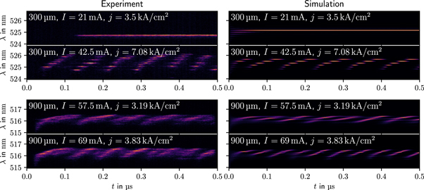
Figure 1. Comparison of measured (left) and simulated (right) streak camera images. The first two rows show data for the diode with a cavity length of  and different currents, while the lower two rows correspond to the diode with a cavity length of
  . For the visualization of the simulation results, the contribution of a mode is given by a gaussian centered at the respective wavelength with a width of
  multiplied by the number of photons in that mode at that point in time.
Download figure:
Standard image High-resolution imageFor currents slightly above threshold the photon density is too small for nonlinear effects such as the asymmetric mode coupling to be relevant. Therefore only the mode with the highest gain will be active, as shown in figure 1 for the  laser diode. The simulation agrees well with the experiments. In order to simulate the differences between separate single-shot measurements, it is possible to include noise due to quantum fluctuations [20–23].

Figure 2. Band structures obtained using the k · p method. The optical matrix elements are also given in terms of their bulk value.
Download figure:
Standard image High-resolution imageThe time between two peaks of the same mode defines the mode rolling frequency. Extracting this for both theory and experiment, figure 3 shows how this frequency depends on the current density. Here simulation agrees well with the experiment for the  laser diode. Using the same parameters, the mode rolling frequencies for the
  laser diode are too high, but show the same trends as observed in the experiment. Better agreement can be obtained, for example, by changing the scattering time to
  , as shown in figure 3. While changing free parameters such as the scattering time or the dephasing constant has an effect on the mode dynamics, the resulting mode rolling frequencies remain in the megahertz range.

Figure 3. Mode rolling frequency as a function of the current density. Determined by the average time between two peaks in the streak camera images.
Download figure:
Standard image High-resolution image
As discussed above, for currents immediately above threshold there is only one lasing mode and no mode rolling frequency can be defined. This is displayed for the  laser diode in figure 1, yet the phenomenon also exists in the longer diode. In this case, however, because of the stronger asymmetric coupling due to a smaller frequency difference between neighboring longitudinal modes, the one-mode-region has a smaller extension.
5. Conclusion
In this publication we presented streak camera measurements of the dynamics of two nitride laser diodes with different cavity lengths. Both show a rich mode dynamics including mode rolling effects, which can be explained by beating vibrations of the carrier densities in the QWs. This behavior can be modelled by a Maxwell-Bloch equation-based dynamical laser model, showing good agreement to the experiment. The model also offers a microscopic derivation of the asymmetric and symmetric coupling terms used by Yamada [11] in an earlier rate equation model [14]. Due to the smaller separation of longitudinal modes, the  laser diode displays faster mode rolling and more longitudinal modes are involved in the process.