

Abstract
Recent advances in experimental and computational methods are increasing the quantity and complexity of generated data. This massive amount of raw data needs to be stored and interpreted in order to advance the materials science field. Identifying correlations and patterns from large amounts of complex data is being performed by machine learning algorithms for decades. Recently, the materials science community started to invest in these methodologies to extract knowledge and insights from the accumulated data. This review follows a logical sequence starting from density functional theory as the representative instance of electronic structure methods, to the subsequent high-throughput approach, used to generate large amounts of data. Ultimately, data-driven strategies which include data mining, screening, and machine learning techniques, employ the data generated. We show how these approaches to modern computational materials science are being used to uncover complexities and design novel materials with enhanced properties. Finally, we point to the present research problems, challenges, and potential future perspectives of this new exciting field.
Export citation and abstract BibTeX RIS

Original content from this work may be used under the terms of the Creative Commons Attribution 3.0 licence. Any further distribution of this work must maintain attribution to the author(s) and the title of the work, journal citation and DOI.
1. Introduction
In the last three decades, we have witnessed the generation of huge amounts of theoretical and experimental data in several areas of knowledge. Within the field of computational materials science, such abundance of data is possible mainly due to the success of density functional theory (DFT) and the fast development of computational capabilities. On the other hand, advances in instrumentation and electronics have enabled experiments to produce large quantities of results. Therefore, along with the high-throughput (HT) approach, we have obtained a huge number of theoretical as well as experimental data, and the logical next step is the emergence of novel tools capable of extracting knowledge from such data. Among such tools, the field of statistical learning has coined the so-called machine learning (ML) techniques, which are currently steering research into a new data-driven science paradigm.
In this review, we strive to present the historical development, state of the art, and synergy between the concepts of theoretical and computational materials science, and statistical learning. Our choice is to focus on DFT and HT methods for the former and ML for the latter. A chronological evolution of science, with emphasis on the specific area of materials research is presented in section 1. Next, in section 2 we describe the development and current status of the methods used to generate data within the DFT and HT frameworks and analyze it via ML. We also discuss how these ingredients merged into the field of materials informatics (MI). In section 2.1, we chose to discuss DFT, since it has become the cornerstone simulation procedure in theoretical materials science. HT and ML approaches, which are discussed in sections 2.2 and 2.3 respectively, follow a logical sequence. The former is used to generate large amounts of data, while the latter requires the existence of such data in order to extract knowledge from it. In the sequence, in section 3 we review the progress of current research applying those methods to materials science problems, including materials discovery, design, properties, and applications. Finally, in section 4 we discuss an overview and perspectives for future research. A simplified presentation of the topics presented in this work and their complex relationships are summarized in figure 1.

Figure 1. Schematic presentation of the topics discussed in this review and their relationships. The possible atomic combinations form a great number of compounds, which can be studied by means of experimental, theoretical or computational approaches, especially with high-throughput calculations. Large quantities of data generated are then stored in databases, which can be used by means of materials screening or machine learning, both of which leads to promising materials candidates. Data-driven or traditional routes select materials suited for specific applications. We illustrate these relationships in the context of two-dimensional materials. Figures from panels adapted with permission from [1] (experiments) (© 2012 Macmillan Publishers Limited. All rights reserved. With permission of Springer), [2] (computational science and machine learning), and [3] (materials prediction) (© 2018 Macmillan Publishers Limited, part of Springer Nature. All rights reserved. With permission of Springer).
Download figure:
Standard image High-resolution image1.1. Science paradigms: data science
As part of the human endeavor, science is subject to constant reshaping owing to historical circumstances. The present 'data deluge' resulting from advances in information technologies [4] is deeply affecting the way we study science. Experimental, theoretical, and computational sciences are also responsible for generating huge amounts of data and can benefit from a new perspective. Jim Gray, the 1998 Turing award-winner, presented this idea historically in his last presentation:
'Originally, there was just experimental science, and then there was theoretical science, with Kepler's Laws, Newton's Laws of Motion, Maxwell's equations, and so on. Then, for many problems, the theoretical models grew too complicated to solve analytically, and people had to start simulating. These simulations have carried us through much of the last half of the last century. At this point, these simulations are generating a whole lot of data, along with a huge increase in data from the experimental sciences. People now do not actually look through telescopes. Instead, they are 'looking' through large-scale, complex instruments which relay data to datacenters, and only then do they look at the information on their computers.
The world of science has changed, and there is no question about this. The new model is for the data to be captured by instruments or generated by simulations before being processed by software and for the resulting information or knowledge to be stored in computers. Scientists only get to look at their data fairly late in this pipeline. The techniques and technologies for such data-intensive science are so different that it is worth distinguishing data-intensive science from computational science as a new, fourth paradigm for scientific exploration [4].'—Jim Gray, 2007 [5].
The amount of data being generated by experiments and simulations has led us to the fourth paradigm of science over the last years, which is the so-called (big) data-driven science. Such a paradigm naturally follows from the first three paradigms of experiment, theory, and computation/simulation, as shown in figure 2. Its impact in the field of materials science has led to the emergence of the new field of materials informatics. Within this new data-driven point of view, a variety of pieces, such as Big Data and Data Science, come together in order to make possible the extraction of knowledge from data. Big Data is defined as a collection of data which is unfeasible to be processed, searched or analyzed by on-hand database tools due to its large size and complexity. It is characterized by its diverse and huge volume, usually ranging from terabytes to petabytes of data, being created in or near real-time. Such data is found either structured and unstructured in nature, and is exhaustive, usually aiming to capture entire populations in a scalable manner [7]. Simple tasks represent challenges in this scale: capture, curation, storage, search, sharing, analysis, and visualization of the data cannot be accomplished without the proper tools. Thus, it can be effectively summarized by the popular 'five V's': volume, velocity, variety, veracity, and value, shown in figure 3(right). A related sixth V is visualization, although not exclusive to Big Data, which requires different techniques to handle data with various characteristics.

Figure 2. The four science paradigms: empirical, theoretical, computational, and data-driven. Each paradigm both benefits from and contributes to the others. Adapted from [6]. CC BY 4.0
Download figure:
Standard image High-resolution image
Figure 3. (Left) Data Science as an integrative discipline. Adapted from [8]. (Right) Big Data characteristics known as the 'five V's'.
Download figure:
Standard image High-resolution imageStriving to tackle the challenges imposed by Big Data, the field of Data Science has arisen. It is largely interdisciplinary being a combination of mathematics and statistics, computer science and programming, and domain knowledge for problem definition and solving, as shown in figure 3(left). Its objective is, roughly speaking, to deal with the whole process of data production, cleaning, preparation, and finally, analysis. Data science encompasses areas such as Big Data, which deals with large volumes of data, and data mining, which relates to analysis processes to discover patterns and extract knowledge from data, part of the so-called Knowledge Discovery in Databases (KDD).
The analysis process within Data Science is challenging, as the techniques are very different from traditional static and rigid datasets, generated and analyzed under a predetermined hypothesis. The distinction from traditional data is based on the larger abundance, exhaustivity, and variety of Big Data. It is also much more dynamic, messy and uncertain, being highly relational [7]. Recently, the possibility of overcoming such a challenge slowly started to be envisaged due to advances in high-performance computation and discovery of new analytical techniques, enabling one to deal with the complexity and vastness of the data. Originally, these techniques were developed in artificial intelligence (AI) and expert systems fields. Their objective was to produce ML algorithms that could automatically mine and detect patterns, and then build predictive models and optimize outcomes [7]. The number of different algorithms that can be applied to a dataset is huge, which makes possible their performance comparison, thus, letting one choose the best model or explanation, or even a combination of those (ensemble approach). This approach differs from the traditional selection based on knowledge specific to the technique and data. Thus, the set of Big Data and Data Science, or simply Big Data analytics, can be seen as a new epistemological approach, where insights can be 'born from the data'. The contrast with traditional methods of testing a theory by analyzing relevant data (e.g., fit the data to theory) is striking [7].
A new research paradigm is related to the way we produce knowledge. As stated by the philosopher Thomas Kuhn, 'a paradigm constitutes an accepted way of interrogating the world and synthesizing knowledge common to a substantial proportion of researchers in a discipline at any one moment in time' [9]. Periodically, the accepted theories and approaches are challenged by a new way of thinking, and the framework encompassed by Big Data and ML incarnates such paradigm in multiple disciplines.
1.2. Development of computational materials science
Novel materials enable the development of technological applications that are key to overcome challenges faced by society. Even though the impact of materials discovery throughout history is hard to quantify, ranging from the Stone Age, going through to the Bronze and Iron Ages, up to the modern silicon technologies, their impact is easily grasped [10]. Furthermore, it is estimated that materials development enabled two-thirds of all advancements in computation, and transformed other industries as well, such as energy storage [11].
Time to market for new technologies based on novel materials takes approximately 20 years, while their development can span an even longer period [12]. Moreover, once a material is consolidated for a technology, it is rarely substituted owing to the costs associated with the establishment of large-scale production infrastructure [13]. Silicon in the semiconductor industry is an enduring example of that. Therefore, the introduction of a material for a specific sector is increasingly important for its establishment success, and recently several new technological niches face demands for potential materials.
Given the fast-growing demand for novel materials and relatively slow development of them, at the same time that computational resources and algorithms face huge improvements, it seems almost natural to ask: how can computational science improve the efficiency of materials discovery? Other areas such as the pharmaceutical and biotechnology industries have already given some hints [14, 15]. However, within the fourth data-driven science paradigm, the computational materials community finds itself somehow delayed, in comparison to these fields. This late arrival is related to bottlenecks in computational capability, but since the first materials simulations were carried out, an ever increasing amount of research is taking place within this paradigm. In figure 4, the number of publications indicate this situation. Novel emerging approaches usually face an initial growth driven by over-enthusiasm, followed by a disillusionment due to unmet expectations. Maturity is achieved after this period when robust and steady developments result in realistic expectations and community adoption.

Figure 4. Chronological evolution of the number of publications for DFT, HT, ML, and materials informatics. Initial developments of each discipline date to many decades before actual adoption by the community. Data compiled from the Web of Science platform, using each keyword in the 'Topic' search term.
Download figure:
Standard image High-resolution imageThe field is progressing at a fast pace and according to Allison et al, computational materials design can lead to returns on investment around 300%–700% and in a shorter time framework as well [16]. Accordingly, such a high yield is attracting private and governmental investments in the quest for efficiency. A key step in that sense is the Material Genome Initiative (MGI) [17–19], one of the largest government funding projects which is behind the recent success of several groups in the US. The task to accelerate the time from discovery to commercialization of novel technologies is a central one in MGI.
Traditional approaches to theoretical and computational materials science, termed direct approach, rely on the calculation of properties given the structural and compositional data of materials. Search for candidate materials presenting target properties in this scenario is a tedious process performed case-by-case or by fortuitous sampling of the right example. The search space can be restricted on prior knowledge about similar materials, nonetheless, the search is still a structure and composition to property mapping. This trial and error experimentation has now been complemented and guided by computational science in an attempt to narrow this search space [20].
The sheer massive data generation is no assurance of converting it into information and then to knowledge. Moreover, converting this knowledge for the benefit of society, which is the ultimate goal, is an even larger challenge. In figure 5, Glick [21] represents these ideas as gaps between data creation and storage, and the capability to obtain knowledge and usable technologies. The tendency of this gap is to increase over time. Therefore, usage of data-driven approaches is paramount in order to reduce the gap and advance research given this scenario.

Figure 5. The increasing gap between data, information, knowledge, and utility, which calls for more efficient approaches to accelerate this conversion. Adapted from [21], copyright 2013 with permission from Elsevier.
Download figure:
Standard image High-resolution image2. Fundamentals of methods
Recent advances in experimental and computational methods have resulted in massive quantities of data generated, presenting increasing complexity. Machine learning techniques aim to extract knowledge and insight from this data by identifying its correlations and patterns. Although we focus on computational techniques, the general concepts are not restricted to them. In this section we present the fundamental approaches, following a logical timeline from DFT to HT to ML. As here we focus on materials science research using computational methods, the first topic is DFT. It is a natural choice of representative within the general class of methods used to generate data, due to its widespread use in materials science. Next, the HT approach is presented, where any experimental or computational methodology (such as DFT) can be employed to generate massive amounts of data in an automated fashion. Resulting data, irrespective of its origin, is then used as a substrate to the learning process, within the ML approach, resulting in extraction of knowledge from the patterns discovered.
Considering the historical development of research in computational materials science, we can classify the different problems and methods used to tackle them into three generations related to the topics mentioned above [22]. The first generation is related to materials property attainment given its structure, using local optimization algorithms, usually based on DFT calculations performed one at a time. It is still the most widespread approach, owing to the great improvements enabled by large scale high-throughput calculations. The second generation is related to crystal structure prediction given a fixed composition, using global optimization tasks like genetic and evolutionary algorithms. Such an approach requires a considerable number of calculations to be performed in a systematic manner, thus relying heavily on HT methods. Finally, the third generation is based on statistical learning. It also enables the discovery of novel compositions, besides much faster predictions of properties and crystalline structures given the vast amount of available physical and chemical data via ML algorithms.
2.1. Density functional theory (DFT)
2.1.1. Historical developments
In the first half of the 20th century, with the formulation of Quantum Mechanics, it was possible to understand the microscopic properties of the materials. Much of the empirical models used by chemists, for example, the concept of bond proposed in the Lewis model, appeared in the solution of the Schrödinger equation [23]. However, the precise resolution of that equation when we have systems involving the electron–electron interaction introduces intrinsic difficulties in its solution, leading to the famous remark by Dirac in 1929 [24]: 'The fundamental laws necessary for the mathematical treatment of a large part of physics and the whole of chemistry are thus completely known, and the difficulty lies only in the fact that application of these laws leads to equations that are too complex to be solved'. There was a shift such that major efforts were now needed in computational aspects rather than theoretical ones.
In the late 1920s and early 1930s, when computers were not in use, some approximate methods were born. The goal was to make many-electron systems treatable. Examples are the Hartree model [25], which seeks to obtain the observables via approximate wave function construction and the Thomas–Fermi–Dirac model [26] that attempted to describe the systems via their electronic density. In 1964 Hohenberg and Kohn [27] published an article that became the paradigm for the understanding of materials properties, today known as Density Functional Theory (DFT). The DFT is based on two theorems elegantly demonstrated in [27]. They showed that in a system with N electrons, (i) the external potential V(r), felt by the electrons is a unique functional of the electronic density n(r) and (ii) the ground state energy E[n] is minimal for the exact density. In other words, by knowing the electron density, we can obtain the precise energy of the ground state.

The question of how to write down the density was answered by Kohn and Sham a year later [28]. They proposed the addition of an exchange-correlation term to the energy, Exc[n] capable of mapping the kinetic energy of the interacting electrons T[n] system into a non-interacting picture Ts[n],

where UH is the Hartree potential, and Vext is an external potential. Such new formulation leads to the famous Kohn-Sham (KS) equations,


where  and ϕj are the Lagrange multipliers of the variational problem that leads to the KS equation (equation (3)), usually interpreted as the energy levels of the many-electron system and the Kohn–Sham orbitals respectively, while veff and vxc = δE/δn are referred to the Kohn–Sham effective potential and exchange-correlation potential, respectively. With this set of equations, a self consistent cycle could be envisaged: one starts with a tentative density n(r), plugs in a functional form of vxc and builds the effective potential veff. Next, they obtain the eigenvalues
  j and eigenvectors ϕj of the Kohn–Sham equations. The electronic density is obtained then from the set of ϕj and the process is repeated until a convergence criteria (usually on the total energy of the system) is reached.
It is important to note that although the work of H–K and K–S was published in the 1960s, the major trust and recognition of its importance came only in the 1980s. This delay in recognition by the community, especially by chemists, occurred mainly for two reasons. The first is the increase in computational capacity available to the scientific community and the second is the continuous development of theoretical methods that have made it possible to deal with more complex problems with more predictive capacity algorithms.
The DFT is formally exact, however, in practice, a series of approximations are required in order to solve the K–S equations. First, one needs to select the exchange-correlation term contained in equation (2). A large variety of functionals can be found in the literature, some parameter-free and other semi-empirical, i.e., containing parameters which are fitted from data. Next, one has to choose how to treat the valence and core electrons. In the early days of DFT, only the so-called all-electron treatment was available, and its drawback was the restriction of systems that could be simulated at that time. However, valence orbitals determine the properties of solids. In 1940, with that in mind, Herring proposed a powerful method for the determination of electronic states in crystalline materials. In Herring's approach, known as orthogonalized plane waves (OPW), an orbital base is proposed as a linear combination of core states and plane waves [29]. From the formal point of view, it was a success, but it presented severe problems of convergence due to the need to orthogonalize the plane waves with the orbitals of the core states. Phillips and Kleinman elegantly solved this inconvenience. They showed that it is possible to obtain the same eigenvalues from the secular equation of the OPW method in an effortless way known as the pseudopotential method [30].
The pseudopotential method led to the possibility of simulation of the whole periodic table. Such a method basically describes the core electrons and corresponding nuclei in a simplified manner, by means of an effective potential which the valence electrons are subject to. Some popular approaches are the projector augmented waves (PAW) [31], norm-conserving and ultrasoft pseudopotentials as developed by Troullier and Martins [32] and Vanderbilt [33]. These approximations reach accuracy comparable to all-electron methods [34]. Therefore, in the 1970s the pseudopotentials ab initio methods became the most powerful tool for accurate description of many-electron systems.
Another important advance in DFT was the treatment of materials imposing links on translational symmetry, via Bloch's theorem [35], known at the time as 'Large Unit Cell'. This procedure allowed the study of more realistic systems such as surfaces, defects, and impurities in amorphous systems, clusters, etc. Owing to the seminal work by Ihm, Zunger and Cohen [36, 37], the calculation of the total energy was also made possible in early 1980.
2.1.2. Current status
Since its initial development, DFT has evolved from limited calculations capable of providing approximate results to an increasingly accurate and predictive methodology, leading to important contributions in several areas such as materials discovery and design, drug design, solar cells, water splitting materials, etc.
As we mentioned earlier, DFT is an exact formulation. However, we are not fully aware of how the electron–electron interactions contained in the exchange-correlation functional occur. The pursuit of the 'exact' functional is still a subject of research, which is elegantly summarized by Perdew as an analogy to the climbing of the so-called Jacob's ladder of DFT approximations [38]. In its first implementation, DFT codes employed the Local Spin Density approximation (LSDA or simply LDA) for the exchange-correlation functional, described by the corresponding energy,

where  are the uniform spin densities of an electron gas, and
  is the exchange-correlation energy per electron of that system. The LDA was very successful in describing systems where the electronic density varies slowly, such as bulk metals, and was in great part responsible for the growing popularity of DFT methods among physicists during the 1970s. On the other hand, the chemistry community did not embrace LDA due to a few systematic errors, such as overestimation of molecular atomization energies and overestimation of bond lengths. Such shortcomings were alleviated in great part when the generalized gradient approximation (GGA) was introduced in the 1980s. In this approximation, the exchange-correlation energy is rewritten taking into account not only the spin densities but also their spatial variation,

where  is the GGA corresponding energy density. One interesting characteristic of the GGA approximation is that it does not require any particular functional form of the exchange-correlation energy density. In fact, only a number of constraints are imposed in the construction of GGA functionals. Owing to that, a number of flavours of exchange-correlation functionals within this approximation are available, namely the Perdew-Burke-Ernzerhof (PBE) [39], Perdew-Wang (PW91) [40], and Becke-Lee-Yang-Parr (BLYP) [41, 42] are some examples of very successful functionals.
The next step in the complexity of exchange-correlation functionals is usually referred to as the advent of the meta-GGA approximation. Their new ingredient is the introduction of the so-called Kohn–Sham kinetic energy density  ,
,

where the implicit dependence of the kinetic energy on the spin density should be noted, i.e., ![${\tau }_{\uparrow /\downarrow }={\tau }_{\uparrow /\downarrow }\left[{n}_{\uparrow /\downarrow }({\bf{r}})\right]$](https://content.cld.iop.org/journals/2515-7639/2/3/032001/revision2/jpmaterab084bieqn6.gif) . Meta-GGA approximation represented an improvement over many issues known to plague GGA functionals, for example, delivering better atomization energies as well as metal surface energies. Popular functionals within this approximation comprise the Tao–Perdew–Staroverov–Scuseria functional (TPSS) [43], and the more recent proposal of the non-empirical strongly constrained and appropriately normed (SCAN) functional of Sun et al [44]. Successful attempts of semilocal functionals for improved bandgaps of different materials include the Tran–Blaha modified Becke–Johnson (mBJ) [45] and ACBN0 functionals [46, 47].
. Meta-GGA approximation represented an improvement over many issues known to plague GGA functionals, for example, delivering better atomization energies as well as metal surface energies. Popular functionals within this approximation comprise the Tao–Perdew–Staroverov–Scuseria functional (TPSS) [43], and the more recent proposal of the non-empirical strongly constrained and appropriately normed (SCAN) functional of Sun et al [44]. Successful attempts of semilocal functionals for improved bandgaps of different materials include the Tran–Blaha modified Becke–Johnson (mBJ) [45] and ACBN0 functionals [46, 47].
Up to this point in the Jacob's ladder of DFT approximations one can find only local (LDA) or semilocal (GGA and meta-GGA) functionals of the density. Representing a step further, a proposal inspired by the Hartree–Fock formulation introduced non-locality in DFT by mixing a fraction of the exact exchange term

into the exchange-correlation energy within the GGA,

where α ∈ [0, 1] is a mixing parameter, usually chosen in the range between 0.15 and 0.25. Such an approach is known as hybrid functional, which partially mended a serious problem of materials band-gap underestimation known to plague GGA functionals. Its main shortcoming is the computational requirements, as the calculation of the non-local term in equation (9) is an intensive task, once it involves the exchange of each orbital ϕj with all other orbitals in the system. Nonetheless, some hybrid functionals were widely adopted in both the solid state physics as well as quantum chemistry communities. Examples are the PBE0 [48, 49] and the Coulomb interaction screened Heyd–Scuseria–Ernzerhof (HSE) [50] hybrid functionals based on the PBE Exc and the B3LYP functional [42, 51], which introduced mixing as well as other empirical parameters into its precursor BLYP.
Finally, by considering both occupied and unoccupied orbitals in the theory, one reaches what could be considered the furthermost degree of complexity of DFT. Within this level of approximation, one finds the Random Phase Approximation (RPA) [52, 53], which can successfully account for electronic correlation.
The landscape of DFT applications and tools is very wide, and many features have been made available for ab initio calculations of a large number of systems. Total energy calculations, potential energy evaluation and obtention of the energy spectra of both crystalline structures as well as molecules and organic complexes can be obtained in a straightforward way using DFT methods. Metals, semiconductors, and insulators can have their band structure routinely scrutinized by means of plane-wave based implementations of the DFT equations, by solving the KS equations in the reciprocal or electron momentum space. Thus, effective masses of both electrons and holes, as well as band gaps and optical transitions are available from DFT. Structural properties include stress tensors, bulk modulus, and phonon spectra, which can help identify the structural stability of materials. Dispersion interaction is not an intrinsic ingredient within LSDA or GGA. However, many parametrized models of such forces have been included into DFT codes [54–57], allowing a good description of non-covalent bonding between molecules.
A fundamental limitation of DFT arises from its mathematical construction: it works only for the ground state density. Thus, the study of excited states is hindered within this method, even though workarounds such as time-dependent DFT (TDDFT) [58–60] have been proposed. Moreover, despite the fact that they usually are interpreted as physical quantities, the KS eigenvalues and eigenvectors do not correspond, at least formally, to the energy levels and eigenstates of the system, respectively. Strongly correlated systems, such as d electrons in transition metal oxides, also have to be tackled with auxiliary theories such as the Hubbard U parameter [61, 62]. Many other methods which are usually referred to as post-KS have been proposed in order to overcome DFT deficiencies. The GW approximation [63, 64], and the solution of the Bethe-Salpeter equation for exciton dynamics [65, 66], among other methods are famous examples. Moreover, strongly correlated phenomena, which is not captured by the standard DFT approach are now being investigated using the Dynamical Mean Field Theory (DMFT) [67, 68]. Which can be integrated into the DFT self-consistent cycle [69], or used in post-processing level [70]. However, the greater precision delivered by such methods is accompanied by greater computational demands, hindering the widespread use of these algorithms. Roughly speaking, a scaling law of  impedes the application of DFT calculations for very large systems (presently, N > 1000s atoms). Linear scaling
  methods [71, 72] enable the calculation of much larger systems, currently up to 106s atoms [73].
An important strategy to extend beyond the capabilities of the DFT method is to use auxiliary codes. For example, quantities that require large reciprocal space sampling, such as electrical conductivity, spin Hall conductivity (SHC), Anomalous Hall conductivity (AHC), to cite a few, are cumbersome to obtain. The electrical conductivity can be calculated using interpolation methods based on DFT calculations implemented in BoltzTraP, BoltzWann, ShengBTE, and PAOFLOW [74–77]. PAOFLOW can also calculate SHC, AHC, Fermi surfaces, topological invariants, and other properties. Topological invariants are also calculated in DFT using Z2Pack [78] and Wannier Tools [79] which are integrated into many different DFT codes. Investigation of ballistic transport phenomena is possible via SIESTA-based codes [80], namely the TranSIESTA [81], TRANSAMPA [82], and Smeagol [83] packages. Excitation properties can also be addressed with YAMBO [84], and BerkeleyGW [85]. The vibrational properties are mainly obtained via perturbation theory or the finite displacement approach. The first is not general and is implemented primarily in Quantum Espresso. The second approach is compatible with several DFT codes that can optimize crystal structures. Nevertheless, they are very computational-demanding, due to the large supercells involved. The Phonopy code is a helpful resource to obtain vibration related quantities such as phonon band structure and density of states, dynamic structure factor, and Grüneisen parameters [86].
In summary, DFT is a mature theory which is currently the undisputed choice of method for electronic structure calculations. A number of papers and reviews are presented in the literature [87–92], facilitating the widespread of the theory and, thus, the entry of researchers into the field of computational solid state physics, materials science, and quantum chemistry. Although the implementations of DFT take place in many codes and scopes (see table 1), it has been shown recently that the results are consistent as a whole [34].
Table 1. Selection of DFT codes according to their basis types. GPL stands for GNU public license.
| Name | License | Reference |
|---|---|---|
| Plane-waves basis sets | ||
| VASP | commerciala | [93–96] |
| Quantum Espresso | GPL | [97, 98] |
| CASTEP | commercialb | [99, 100] |
| ABINIT | GPL | [101–103] |
| CP2Kd | GPL | [104–108] |
| CPMD | free | [109–111] |
| ONETEP | commercial | [112] |
| BigDFT | GPL | [113] |
| Atom-centered basis sets | ||
| Gaussian | commercial | [114] |
| GAMESS | free | [115, 116] |
| Molpro | commercial | [117] |
| SIESTA | GPL | [80] |
| Turbomole | commercial | [118] |
| ORCA | freec | [119] |
| CRYSTAL | commercialb | [120] |
| Q-Chem | commercial | [121] |
| FHI-aims | commercial | [122] |
| Real-space grids | ||
| octopus | GPL | [123–125] |
| GPAWe | GPL | [126, 127] |
| Linearized augmented plane waves | ||
| WIEN2k | commercial | [128] |
| exciting | GPL | [129] |
| FLEUR | MIT | [130] |
aFree for academic institutions in Austria. bFree for academic institutions in UK. cFor academics. dCP2K employs mixed plane-waves and atom-centered basis sets. eGPAW can also employ plane-waves or atom-centered basis sets.
2.1.2.1. Structure prediction
DFT calculations provide a reliable method to study materials once the crystalline or molecular structure is known. Based on the Hellman–Feynman theorem [131], one can use DFT calculations to find a local structural minima of materials and molecules. However, a global optimization of such systems is a much more involved process. The possible number of structures for a system containing N atoms inside a box of volume V is huge, given by the combinatorial expression

where δ is the side of a discrete box which partitions the volume V and ni is the number of atomic species i in the compound. This number becomes very large (≈10N) even for small systems (N < 20) and large discretization box (δ = 1 Å). In order to probe such potential energy surface, one has to visit states in a 3N + 3 dimensional space ( degrees of freedom for atomic positions and 6 degrees of freedom for the lattice constants) and assess their feasibility, usually by calculating the total energy in that particular configuration. This is a global optimization problem in a high-dimensional space, which has been tackled by several authors. Here we discuss two of the most popular methods proposed in the literature, namely evolutionary algorithms and basin hopping optimization.
Owing to the fact that not all configurations in this landscape are physically acceptable (i.e. there might be too close pairs of atoms) and some of these are more feasible, some authors realized that the search space should be restricted somehow. One way of achieving such restriction is by means of evolutionary algorithms, where the survival of the fittest candidate structures is taken into account, thus restricting the search to a small region of the configurational space. Introducing mating operations between pairs of candidate structures and mutation operators on single samples, a series of generations of candidate structures is created, and in each of these series only the fittest candidates survive. The search is optimized by allowing local relaxation, via DFT or molecular dynamics (MD) calculations, of the candidate structures, thus avoiding nonphysical configurations, such as too short bond lengths. Evolutionary algorithms have been used to find new materials, such as a new high-pressure phase of Na [132–134].
Another popular method of theoretical structure prediction is basin hopping [135, 136]. In this approach, the optimization starts with a random structure that is deformed randomly given a threshold, which is in turn brought to an energy minima, via e.g. DFT calculations. If the reached minima are distinct from the previous configuration, the Metropolis criterion [137] is used to decide if the move is accepted or not. If the answer is yes, it is said that the system hopped between neighboring basins. Owing to the fact that distinct basins represent distinct local structural minima, this algorithm probes the configurational space in an efficient way.
Other methods of global optimization and theoretical structure prediction of molecules and materials comprise random structure searching (AIRSS) [138], particle-swarm optimization methods [139, 140], parallel tempering, minima hopping [141], and simulated annealing.
The so-called Inverse Design, is an inversion of the traditional direct approach, discussed in section 1.2. Strategies for direct design usually fall into three categories: descriptive, which in general interpret or confirm experimental evidence; predictive, which predicts novel materials or properties; or predictive for a material class, which predicts novel functionalities by sweeping the candidate compound space. The inverse mapping, from target properties to the material was proposed by Zunger [142] as a means to drive materials discovery presenting specific functionalities. According to his inverse design framework, one could find the desired property in known materials, as well as discover new materials while searching for the functionality. This can be seen as another global optimization task, but instead of finding the minimum energy structure, it searches for the structure that maximizes the target functionality (figure of merit). This can be done in three ways: (i) search for a global minimum using local optimization methods, e.g. evolutionary algorithms, aimed to select best fitted candidates based on the property of interest, (ii) materials database querying and subsequent hierarchical screening based on design principles of properties in order to uncover properties in known compounds (materials screening is discussed in section 2.2.1), and (iii) screening of novel compounds obtained by high-throughput calculations (section 2.2) of the convex hull of stable compositions. A number of examples have been reported as a successful application of inverse design principles, such as the discovery of non-toxic, high efficient halide perovskites solar absorbers [143].
2.2. High-throughput (HT)
As discussed in section 2, great advances in simulation methods occurred in the last decades. At the same time, even greater evolution was observed in computational science and technologies. Therefore, as time progresses the computational capacity is rapidly increasing. This results in a major reduction in the time used to perform calculations, so a relatively larger time is spent on simulations setup and analysis. This changed the theoretical workflow and led to new research strategies. Instead of performing many manually-prepared simulations, one can now automate the input creation and perform several (even millions) simulations in parallel or sequentially. This development is presented in figure 6 and the approach is called high-throughput [144].

Figure 6. Time spent for calculations (and similarly for experiments) as a function of technological developments. With the computer technological advances, the calculation step can be less time consuming than the setup construction and the results analysis. Adapted from [145]. Copyright © 2018 American Chemical Society.
Download figure:
Standard image High-resolution imageThe idea is to generate and store large quantities of thermodynamic and electronic properties by means of either simulations or experiments for both existing and hypothetical materials, and then perform the discovery or selection of materials with desired properties from these databases [13]. This approach does not necessarily involve ML, however, there is an increasing tendency to combine these two methodologies in materials science, as already shown in figure 1. Importantly, the HT approach is compatible with theoretical, computational, and experimental methodologies. The main hindrance of a given method is the time necessary to perform a single calculation or measurement. The HT engine has to be fast and accurate in order to produce massive amounts of data in a reasonable time, otherwise, its purpose is lost. Despite the HT generality, here we are mainly interested in its use in the context of first principles DFT calculations and its adapted strategies, discussed in section 2.
The implementation of HT-DFT methods is usually performed in three main steps: (i) thermodynamic or electronic structure calculations for a large number of synthesized and hypothetical materials; (ii) systematic information storage in databases and; (iii) materials characterization and selection: data analysis to select novel materials or extract new physical insight [13]. The great interest in the use of this methodology, the strong diffusion of methods and algorithms for data processing, and the wide acceptance of ML as a new paradigm of science, have resulted in intensive implementation work to create codes to manage calculations and simulations, as well as materials repositories that allow sharing and distributing results obtained in these simulations, i.e., steps (i) and (ii). In general, this is performed in high-performance computers (HPC) with multi-level parallel architectures managing hundreds of simulations at once. A principled way for database construction and dissemination related to step (ii) is the FAIR concept, which stands for findable, accessible, interoperable, and reusable [146, 147]. Meanwhile, item (iii) usually referred to as materials screening or high-throughput virtual screening, is performed via filtering the properties provided by the materials repositories. In a certain way, this could represent a difficulty, since the information provided by the repositories does not necessarily contain the properties of interest, requiring that each research group perform their own HT calculations, which in many cases results in updates of the databases. Thus, in recent years, there has been a considerable increase of materials databases. Examples of such databases are the AFLOWLIB consortium [148], Materials Project [149], OQMD [150], NOMAD [151], and others. In table 2 the most used HT theoretical and experimental databases are presented with a brief description.
Table 2. High-Throughput databases, codes, and tools according to source and purpose. We define a complete package for HT as a multi-engine code that can generate, manipulate, manage and analyze the simulation results.
| Name | Description | URL | Reference |
|---|---|---|---|
| HT databases | |||
| ICSD | Inorganic experimental | http://www2.fiz-karlsruhe.de/icsd_home.html | [152] |
| COD | Organic and Inorganic experimental | http://crystallography.net | [153] |
| AFLOWlib | Multi-purpose repository | http://aflowlib.org/ | [148] |
| Materials Project | Multi-purpose repository | https://materialsproject.org/ | [149] |
| OQDM | Multi-purpose repository | http://oqmd.org/ | [150] |
| CMR | Multi-purpose (3D and 2D materials) repository | https://cmr.fysik.dtu.dk/ | [154] |
| OMDB | Organic materials database | https://omdb.mathub.io/ | [155] |
| MaterialsWeb | 2D materials (derived from Materials Project) | https://materialsweb.org/twodmaterials | [156] |
| JARVIS-DFT | 2D materials | https://ctcms.nist.gov/~knc6/JVASP.html | [157, 158] |
| NOMAD | Multiple source repository | https://repository.nomad-coe.eu/ | |
| Materials Cloud | Multiple source repository | https://materialscloud.org/discover | [3] |
| Citrination | Multiple source (experimental and theoretical) repository | https://citrination.com | [159] |
| Clean Energy Project | Multiple source repository for solar cells | [160] | |
| C2DB | 2D materials (derived from CMR) | https://cmr.fysik.dtu.dk/c2db/c2db.html | [161] |
| HT Codes and tools | |||
| ASE | Complete package for HT | https://wiki.fysik.dtu.dk/ase/ | [162] |
| Pymatgen | Complete package for HT | http://pymatgen.org/ | [163] |
| AiiDA | Framework for HT | http://aiida.net/ | [164] |
| AFLOWπ | Framework for HT | http://aflowlib.org/src/aflowpi/index.html | [165] |
| Atomate | Complete package for HT | https://atomate.org/ | [166] |
| Pylada | Framework for HT | http://pylada.github.io/pylada/ | |
| MPInterfaces | Framework for interfaces HT | http://henniggroup.github.io/MPInterfaces/ | [167] |
| Imeall | Atomistic properties of grain boundaries | https://github.com/Montmorency/imeall | [168] |
| FireWorks | Framework for HT | https://materialsproject.github.io/fireworks/ | [169] |
On the other hand, the profusion of experimental materials databases is less diverse. In this area, we can highlight the Inorganic Crystal Structure Database (ICSD) [152] and crystallographic open database (COD) [153], with ≈200.000 and ≈400.000 crystal structures entries, respectively. The main difference between the two databases is the inclusion of organic, metal-organic compounds and minerals in the COD database.
Despite the complexities involved in steps (i) and (ii), the third step is more significant. In (iii) the researcher inquiries the database in order to discover novel materials with a given property, to gain insight on how to modify an existent one, or to extract a subset of materials for further investigations, which involves more calculations or not. The quality of the inquiry will determine the success of the search. This is usually performed via a constraint filter or a descriptor, which will be used to separate the materials with the desired property, or a proxy variable. We extend the discussion of this process in the next section.
2.2.1. (Big data) Screening and mining
Materials screening or mining can be seen as an integral part of a HT workflow, but here we highlight it as a step on its own. In a rigorous definition, HT concerns the high-volume data generation step, whereas screening or mining process refers to the application of constraints to the database in order to filter or select the best candidates according to the desired attributes. The database is generally screened in sequence through a funnel-like approach, where materials satisfying each constraint pass to the next step, while those who fail to meet one or more of them are eliminated [21]. A final step may be to evaluate what characteristics make the top candidates perform best in the desired property, and then predict if these features can be improved further. Thus, every material who satisfied the various criteria can be optionally ranked according to a problem-defined merit figure, and then this subgroup of selected materials can be additionally investigated or used in applications.
The constraints can be descriptors derived from ML processes or filters guided by the previous understanding of the phenomena and properties, or even guided by human intuition. Traditionally, descriptors construction requires an intimate knowledge of the problem. The descriptor can be as simple as the free energy of hydrogen adsorbed on a surface, which is a reasonable predictor of good metal alloys for hydrogen catalysis [170]. Or more complex such as the variational ratio of spin-orbit distortion versus non-spin-orbit derivative strain, which was used to predict new topological insulators using the AFLOWLIB database [171]. Although materials screening procedure has as its final objective the materials prediction and selection, more complex properties, e.g. that depend on specific symmetries, require direct interaction between ML and materials screening, as represented in figure 1. Specifically, the filters used for the screening can be descriptors obtained via ML techniques. In section 2.3.3.1 we discuss descriptors of increasing complexity degree. In the same way, the ML process can, in turn, depend on an initial selection of materials. This initial step is to restrict the data set exclusively to materials that potentially exhibit the property of interest. For example, in the prediction of topological insulators protected by the time-reversal symmetry, compounds featuring a non-zero magnetic moment are excluded from the database, as we discuss in section 3.2.4.
In figure 7, the materials screening process is schematically presented. As discussed, the first step consists in defining the design principles, i.e., the filters, which can be ML descriptors, theoretical models functions, or materials properties. Subsequently, these filters are used following a funnel procedure. In the ideal scenario, the filters must be applied in a hierarchical way if possible, since this could give information about the mechanisms behind the materials properties. Finally, the materials must be organized according to their performance, i.e., those that exhibit extreme values of the desired behavior. After passing through the filters, if there are candidates that satisfy the criteria, a set of selected materials will be obtained, which could lead to novel technological or scientific applications.

Figure 7. The materials screening process as a systematic materials selection strategy based on constraints filters.
Download figure:
Standard image High-resolution image2.3. Machine learning (ML)
Having presented the most used approaches used to generate large volumes of data, now we examine the next step of dealing and extracting knowledge from the information obtained. Exploring the evolution of the fourth paradigm of science, a parallel can be made between the 1960 Wigner's paper 'The Unreasonable Effectiveness of Mathematics in the Natural Sciences' [172] to the nowadays 'The Unreasonable Effectiveness of Data' [173]. What makes this unreasonable effectiveness of data in recent times? A case can be made for the fifth 'V' of big data (figure 3): extracting value from the large quantity of data accumulated. How is this accomplished? Through machine learning techniques which can identify relationships in the data, however complex they might be, even for arbitrarily high-dimensional spaces, inaccessible for human reasoning.
ML can be defined as a class of methods for automated data analysis, which are capable of detecting patterns in data. These extracted patterns can be used to predict unknown data or to assist in decision-making processes under uncertainty [174]. The traditional definition states that the machine learning, i.e. progressive performance improvement on a task directed by available data, takes place without being explicitly programmed [175]. This research field evolved from the broader area of artificial intelligence (AI), inspired by the 1950s developments in statistics, computer science and technology, and neuroscience. Figure 8 shows the hierarchical relationship between the broader AI area and ML.

Figure 8. Hierarchical description and techniques examples of artificial intelligence and its machine learning and deep learning sub-fields.
Download figure:
Standard image High-resolution imageMuch of the learning algorithms developed have been applied in areas as diverse as finances, navigation control and locomotion, speech processing, game playing, computer vision, personality profiling, bioinformatics, and many others. In contrast, an AI loose definition is any technique that enables computers to mimic human intelligence. This can be achieved not only by ML, but also by 'less intelligent' rigid strategies such as decision trees, if-then rules, knowledge bases, and computer logic. Recently, an ML subfield that is increasingly gaining attention due to its successes in several areas is deep learning (DL) [176]. It is a kind of representation learning loosely inspired by biological neural networks, having multiple layers between its input and output layers.
A closely related field and very important component of ML is the source of data that will allow the algorithms to learn from. This is the field of data science, which we introduced in section 1.1 and figure 3(left).
2.3.1. Types of machine learning problems
Formally, the learning problem can be described [177] by: given a known set X, predict or approximate the unknown function y = f(X). The set X is named feature space and an element x from it is called a feature (or attribute) vector, or simply an input. With the learned approximate function  , the model can then predict the output for unknown examples outside the training data, and its ability to do so is called generalization of the model. There are a few categories of ML problems based on the types of inputs and outputs handled, the two main ones are supervised and unsupervised learning.
In unsupervised learning, also known as descriptive, the goal is to find structure in the data given only unlabeled inputs  , in which the output is unknown. If f(X) is finite, the learning is called clustering, which groups data in a (known or unknown) number of clusters by the similarity in its features. On the other hand, if f(X) is in
  , the learning is called density estimation, which learns the features marginal distribution. Another important type of unsupervised learning is dimensionality reduction, which compresses the number of input variables for representing the data, useful when f(X) has high dimensionality and therefore a complex data structure to detect patterns.
In contrast, in predictive or supervised learning the goal is to learn the function that leads inputs to outputs, given a set of labeled data (xi, yi) ∈ (X , f(X)), known as the training set (contrary to an unknown test set), with i = N number of examples. If the output yi type is a categorical or nominal finite set (for example, metal or insulator), it is called a classification problem, which predicts the class label for unknown samples. Else, if the outputs are continuous real-valued scalars  , it is then called a regression problem, which will predict the output values for the unknown examples. These types of problems and their related algorithms which we introduce in section 2.3.2 are summarized in figure 9. Other types of ML problems are the semi-supervised learning, where a large number of unlabeled data is combined with a small number of labeled ones, multi-task and transfer learning, where information from related problems are exploited to improve the learning task (usually one with little data available [178]), and the called reinforcement learning, in which no input/output is given, but feedback on decisions as means to maximize a reward signal toward learning desired actions in an environment.

Figure 9. Machine learning algorithms and usage diagram, divided into the main types of problems: unsupervised (dimensionality reduction and clustering) and supervised (classification and regression) learning. Adapted from [179], copyright © SAS Institute Inc., Cary, NC, USA. All Rights Reserved. Used with permission.
Download figure:
Standard image High-resolution imageA typical ML workflow can be summarized as follows [180]:
- (i)Data collection and curation: generating and selecting the relevant and useful subset of available data to the problem-solving.
- (ii)Data preprocessing: understandable presentation of data consisting of formatting to a proper format, cleaning corrupt and missing data, transform data as needed by normalizing, discretizing, averaging, smoothing, or differentiating, uniform conversion to integers, doubles, or strings, and proper sampling to optimize representativeness of the set.
- (iii)Data representation and transformation: choose and transform the input data (often a table) to the problem at hand by feature engineering such as scaling, decomposition, or a combination. Especially for materials science applications, this is an important issue which we discuss in section 2.3.3.1.
- (iv)Learning algorithm training: from the previous step, split the dataset into 3 sets: training, validation, and testing datasets. The first one is used in the learning process, where the model parameters are obtained. This step is usually not necessary for unsupervised learning tasks.
- (v)Model testing and optimization: evaluate effectiveness and performance, by means of the validation set. Parameters that cannot be learned (the so-called hyperparameters) are to be optimized using this dataset. Once an optimal set of parameters is obtained, the test set is used in order to assess the performance of the model. If the obtained model is unsuccessful, the previous steps are repeated with improved data selection, representation, transformation, sampling, and removing outliers, or by changing the algorithm altogether.
- (vi)Applications: using the validated model to make predictions on unknown data. The model can be continually retrained whenever new data is available.
In the present context of materials science, we explore the steps: (i) data collection in sections 2.1 to 2.1.2.1, related to any method used to generate data, whether experimental or theoretical, and also show critical examples in section 3.1.1; (iii) data representation and transformation in section 2.3.3.1, discussing how to represent materials in increasing degrees of complexity; (iv) learning algorithms in the next section 2.3.2, presenting the most common and useful algorithms for the different types of ML problems; and (vi) applications in the whole section 3.2, showing the progress, challenges, and perspectives in ML applications to materials science research.
2.3.2. Learning algorithms
According to the 'No Free Lunch Theorems' [181, 182], no ML algorithm is universally superior. Thus, the task of constructing such an algorithm is a case-by-case study. In particular, the choice of the learning algorithm is a key step in building an ML pipeline, and many choices are available, each suited for a particular problem and/or dataset. Such dataset can be of two types: either labeled or unlabeled. In the first case, the task at hand is to find the mapping between data points and corresponding labels  by means of a supervised learning algorithm. On the other hand, if no labels are present in the dataset, the task is to find a structure within the data, and unsupervised learning takes place.
Owing to the large abundance of data, one can easily obtain feature vectors of overwhelmingly large size, leading to what is referred to as 'the curse of dimensionality'. As an example, imagine an ML algorithm that receives as input images of n × n greyscale pixels, each one represented as a numeric value. In this case, the matrix containing these number is flattened into an array of length n2 which is the feature vector, describing a point in a high dimensional space. Due to the exponential dependency, a huge number of dimensions is easily reachable for average sized images. Memory or processing power become limiting factors in this scenario.
A key point is that within the high-dimensional data cloud spanned by the dataset, one might find a lower dimensional structure. The set of points can be projected into a hyperplane or manifold, reducing its dimensionality while preserving most of the information contained in the original data cloud. A number of procedures with that aim, such as principal component analysis (PCA) in conjunction with single value decomposition (SVD) are routinely employed in ML algorithms [183]. In a few words, PCA is a rotation of each axis of the coordinate system of the space where the data points reside, leading to the maximization of the variance along these axes. The way to find out where the new axis should point to is by obtaining the eigenvector corresponding to the largest eigenvalue of the XTX, where X is the data matrix. Once the largest variance eigenvector, also referred to as the principal component, is found, data points are projected into it, resulting in a compression of the data, as is depicted in figure 10.

Figure 10. Principal component analysis (PCA) performed over a 3D dataset with 3 labels given by the color code (left) resulting in a 2D dataset (right).
Download figure:
Standard image High-resolution imageA variety of ML methods is available for unsupervised learning. One of the most popular methods is k-means [184], which is widely used to find classes within the dataset. k-means consists of an algorithm capable of clustering n data points into k subgroups (k < n) by direct calculation of points distances with respect to each groups' centroid. Once the number of centroids (k) is chosen and their starting position is selected ( ), e.g. randomly selected, the algorithm iterates over two steps. First, the distances of the data points to each centroid are calculated, and the points are labeled y(i) as belonging to the subgroup corresponding to the closest centroid. Next, a new set of centroids (
 ) is computed by averaging the positions of the class members of each group. The two steps are described by equations (12) and (13),


where  represents the choice of the metric (being p = 2, the Euclidean metric the most popular), nj is the number of points assigned to cluster with centroid
  , δn,m is the Kronecker delta function, which is 1 if m = n or zero otherwise, and t is the iteration step index. Convergence is reached when no change in the assigned labels is observed. The choice of the starting positions for the centroids is a source of problems in k-means clustering, leading to different final clusters depending on the initial configuration. A common practice is to run the clustering algorithm several times and consider the final configuration as the most representative clustering.
Hierarchical Clustering is another method employed in unsupervised learning which can be found in two flavors, either agglomerative or divisive. The former can be described by a simple algorithm: one starts with n classes, or clusters, one containing a single example  from the training set, and then measures the dissimilarity d(A, B) between pairs of clusters labeled A and B. The two clusters with the smallest dissimilarity, i.e. more similar, are merged into a new cluster. The process is then repeated recursively until only one cluster, containing all the training set elements, remains. The process can be better visualized by plotting a dendrogram, shown in figure 12. In order to cluster the data into k clusters, 1 < k < n, the user is required to cut the hierarchical structure obtained at some intermediate clustering step. There is certain freedom into choosing the measure of dissimilarity d(A, B), and three main measures are popular. First, the single linkage takes into account the closest pair of cluster members,

where dij is a pair member dissimilarity measure. Second, complete linkage considers the furthest or most dissimilar pair of each cluster,

and finally group averaging clustering considers the average dissimilarity, representing a compromise between the two former measures,

The particular form of dij can also be chosen, usually being considered the Euclidean distance for numerical data. Unless the data at hand is highly clustered, the choice of the dissimilarity measure can result in distinct dendrograms, and thus, distinct clusters.
As the name suggests, divisive clustering performs the opposite operation, starting from a single cluster containing all examples from the data set and divides it recursively in a way that cluster dissimilarity is maximized. Similarly, it requires the user to determine the cut line in order to cluster the data.
In the case where not only the features X but also the labels yi are present in the dataset, one is faced with a supervised learning task. Within this scenario, if the labels are continuous variables, the most used learning algorithm is known as Linear Regression. It is a regression method capable of learning the continuous mapping between the data points and the labels. Its basic assumption is that the data points are normally distributed with respect to a fitted expression,

where the superscript T denotes the transpose of a vector,  is the predicted label, and θ is a vector of parameters. In order to obtain the θ parameters, one plugs a cost function, which is given by a sum of least squares error terms, into the model,

By minimizing the above function with respect to its parameters, one finds the best set of θ for the problem at hand, thus leading to a trained ML model. In this case, a closed-form solution for the parameter vector θ exists

where X is a matrix with each row containing a training set example x(i) and y is the corresponding vector of labels.
Once the ML model is considered trained, its performance can be assessed by a test set, which consists of a smaller sample in comparison to the train set that is not used during training. Two main problems might arise then: (i) if the descriptor vectors present an insufficient number of features, i.e. it is not general enough to capture the trends in the data and the regression model is considered plagued by bias, and (ii) if the descriptor presents too much information, which makes the regression model fit the training data exceedingly well but struggles to generalize to new data, then one says it is suffering from overfitting or variance. Roughly speaking, these are the two extremes of model complexity, which is in turn directly related to the number of parameters of the ML model, as is depicted in figure 11. In this case, the use of a regularization parameter λ usually takes place, in order to decrease in a systematic way the complexity of the model and find the optimum spot.

Figure 11. Bias × variance trade-off. The optimum model complexity is evaluated against the prediction error given by the test set. Adapted with permission from [185].
Download figure:
Standard image High-resolution imageRidge or LASSO Regression are extensions of the linear regression, where a regularization parameter λ is inserted into the cost function

and p denotes the metric in this case: p = 0 is simply the number of non-zero elements (usually not considered a metric formally) in θ while p = 1 is referred to as the Manhattan or taxicab metric, and p = 2 is the standard Euclidean metric. When one uses p = 1, the regression model is LASSO (Least Absolute Shrinkage and Selection Operator), where due to the constraint imposed to the minimization problem, not all features present in the descriptors are considered for the fitting. On the other hand, ridge regression corresponds to p = 2, and the outcome in this case is just the shrinkage of the absolute values of the features, i.e. the features with too large values are penalized, adding to the cost function. In both the LASSO as well as ridge regression, the λ parameter controls the complexity of the model, by decreasing and/or selecting features. Thus, in both cases, it is recommendable to start with a very specialized (or complex) model and use λ to decrease its complexity. The λ parameter however cannot be learned in the same way as θ, being referred to as a hyperparameter that should be fine-tuned by e.g. grid search in order to find the one that maximizes the prediction power without introducing too much bias. One is not restrained to choose a specific metric for the regularization term in equation (20): methods for interpolation, such as elastic net [186, 174], are capable of finding an optimal combination of regularization parameters.
Another class of supervised learning, known as classification algorithms, is broadly used when the dataset is labeled by discrete labels. A very popular algorithm for classification is logistic regression, which can be interpreted as a mapping of the predictions made by linear regression into the [0, 1] interval. Lets suppose that the classification task at hand is to decide if a given data point x(i) belongs to a particular class (y(i) = 1) or not (y(i) = 0). The desired binary prediction can be obtained from

where θ is again a parameter vector, and σ is referred to as the logistic or sigmoid function. As an example, the sigmoid function along with some prediction from a fictitious dataset is presented in figure 12. Usually one considers that data point x(i) belongs to class labeled by y(i) if  , even though the predicted label can be interpreted as a probability
  .
.

Figure 12. (a) Example of the sigmoid function and the classification of negative (red) and positive (blue) examples in logistic regression. The gray arrow points out to the incorrectly classified points in the dataset. (b) A Voronoi diagram depicting the k-means classification algorithm. The data point labels correspond to the distinct colors of the scatter points while the assignment to each cluster, defined by their centroids (black crosses), corresponds to the color patches. (c) A dendrogram explaining the hierarchical clustering algorithm, where the color code is a guide to visualize the clusters, and each vertical line represents a cluster. Horizontal lines denote the merging process of two clusters. The number of cuts between a horizontal line and the cluster lines denotes the number of clusters at a given height, which in the case of the gray dashed line is five. (d) k-nearest neighbors Voronoi diagram showing the data point labels and classification patches as color codes.
Download figure:
Standard image High-resolution imageIn the case of classification, the cost function is obtained from the negative log-likelihood. Thus, obtaining the best parameters θ requires the minimization of the aforementioned quantity, given by

where y(i) and  are the actual and predicted binary labels. A regularization parameter λ can be inserted in equation (22) with the same intent of selecting the features as we used in linear regression earlier. Notice that logistic regression can also be used when the data presents multiple classes. In this case, one should employ the one-versus-all strategy, which consists on training n logistic regression models, one for each class, and predicting the labels using the classifier that presents the highest probability.
By proposing a series of changes in the logistic regression, Cortes and Vapnik introduced one of the most popular ML classification algorithms, support vector machines (SVMs) [187]. Such changes can be summarized by the introduction of the following cost function,

where C is a hyperparameter. Insertion of max(z, 0) into the cost function leads to a maximization of a classification gap containing the decision boundary in the data space. The optimization problem described above can also be interpreted as the minimization of  subject to the constraints
  for all
  belonging to the training set. In this case, the labels y(i) are either +1 or −1, signaling that example i is or is not, respectively, a member of a particular class. In fact, by writing the Lagrangian for this constrained minimization problem, one ends up with an expression that corresponds to the cost function given by equation (23).
One of the most powerful features of SVMs is the kernel trick. It can be proved that the parameter vector θ can be written in terms of the training samples,  . This makes possible to express the decision rule as a function of dot products between data vectors

where b and {αi} are the parameters to be learned. The kernel trick consists into transforming the vectors in the dot products  using a mapping
  that takes the data points into a larger dimensional space, where a decision boundary can be envisaged. Moreover, any transformation that maps the dot product into a vector-pair function has been proven to work similarly to what was described above. A couple of the most popular kernels are the polynomial kernel,
  , and the Gaussian kernel, also known as radial basis function (RBF) kernel,

where σ is a hyperparameter to be adjusted. The Gaussian kernel usage is usually interpreted as a pattern-matching process, by measuring the similarity between data points in high-dimensional space.
Up to this point, all classification algorithms presented are based on discriminative models, where the task is to model the probability of a label given the data points or features  . Another class of algorithm capable of performing the same task, but using a different approach of a generative model, where one aims to learn the probability of the features given the label
  can be derived from the famous Bayes formula for calculation of a posterior probability,

where p(y) is the prior probability, i.e. the probability one infers before any additional knowledge about the problem is presented. By making the assumption that the feature vectors  are conditionally independent given the labels y(i), a very popular ML algorithm, the Naïve Bayes classifier is obtained [188]. Its assumption enables one to rewrite the posterior probability from equation (26) as

where xj are the components of the feature vector x. Usually the denominator in this equation is disregarded since it is a constant for all possible values of y, and the probability is renormalized. The training step for this classifier comprises the tabulation of the priors p(y) for all labels in the training set as well as the conditional probabilities  from the same source. Once trained, the Naïve Bayes algorithm predicts the label y by selecting the largest posterior probability
  over all possible labels y.
Another popular and simple classification algorithm is k-nearest neighbors (kNN). Based on similarity by distance, this algorithm does not require a training step, which makes it attractive for quick tasks. In short, given a training set composed of data points in a d-dimensional space  , kNN calculates the distance between these points and an unseen data point x,

where p = 0, 1, 2, ... is the metric, as discussed earlier in this section. Once all distances are obtained, the class of x is simply the class of the majority of its k nearest neighbors. If there is no majority, its class is assigned randomly from the most frequent labels of the neighbors. On the other hand, a regressor based on kNN is obtained by averaging the continuous label values of the nearest neighbors. As mentioned earlier for other ML algorithms, the value of k cannot be learned in this case, leaving the task of choosing a sensitive k to the user. For classification tasks, different choices of such hyperparameter might result in distinct partitionings of the data cloud, which can be visualized as the Voronoi tessellation diagrams in figure 12.
Finally, some ML algorithms are suited both for classification and regression. Decision Trees are a popular and fast ML algorithm that can be used in both cases. Since it can be implemented in a variety of flavors, we chose to explain briefly the workings of two of the most popular implementations, the classification and regression trees, or CART, and the C4.5 algorithm [189, 190]. Both methods are based on the partitioning of the data space, i.e. the creation of nodes, in order to optimize a certain splitting algorithm. Each node of the tree contains a question which defines such a partition. When no further partitioning of the space is possible, each disjoint subspace, referred to as the leaves, contains the data points one wishes to classify or predict.
C4.5 performs a series of multinary partitioning operations over the training set S. This is done in such a way to maximize the ratio between information gain and potential information that can be obtained from a particular partitioning or test B

where the information gain G(S, B) is

where fi is the relative frequency of elements belonging to class Ci in the training set S, while  is the same relative frequency with respect to a particular partitioning Sj of the training set after performing the test B. The potential information P(S, B) that such partitioning can provide is given by

Partitioning takes place up to the point where the nodes contain only examples of one class or examples of distinct classes that cannot be distinguished by their attributes.
On the other hand, CART is a decision tree method which is capable of binary partitioning only. In the case of classification tasks, it uses a criterion for splitting which is based on the minimization of the Gini impurity coefficient

where S is the training set and fj is the relative frequency of member of the j-th class in this set. If one is interested in using CART for a regression task, there are two main differences to be considered. First, the nodes predict real numbers instead of classes. Second, the splitting criterion, in this case, is the minimization of the resubstitution estimate, which is basically a mean squared error

where yi is the label of the i-th example while  is the corresponding predicted value. The consequence of such partitioning is that for each partition, the predicted value is the average of the values within that partition. Thus, CART outputs a piecewise constant function for regression.
One of the major issues with regression trees is that once they are trained, most of the time they suffer from overfitting. A couple of strategies to overcome this problem have been proposed, such as pruning the trees' structures in order to increase its generalization power, loosing however some of their accuracies. More advanced methods include Random Forests, which is an ensemble method based on training several decision trees and averaging their predictions [191]. In this case, the trees are smaller versions of the structures described previously, trained using a randomly chosen subset of the features of the dataset, and usually a bootstrap sample of the same set. In some sense, building a series of weaker learners and combining their predictions enables the algorithm to learn particular features of the dataset and better generalize to new, unseen data.
Artificial Neural Networks (ANNs) corresponds to a class of algorithms that were, at least in their early stages, inspired by the brain structure. An ANN can be described as a directed weighted graph, i.e, a structure composed of layers containing processing units called neurons, which are in turn connected to other such layers, as depicted in figure 13. Many kinds of ANNs are used for a variety of tasks, namely regression, and classification, and some of the most popular architectures for such networks are feed-forward, recurrent, and convolutional ANNs. The main difference between these architectures is basically on the connection patterns and operations that their neurons perform on data.

Figure 13. Example of a feed-forward ANN with N hidden layers and a single neuron in the output layer. Red neurons represent sigmoid activated units (see equation (35)) while yellow ones correspond to the ReLU activation (equation (37)).
Download figure:
Standard image High-resolution imageTypically in an ANN, an input layer receives the descriptor vectors from the training set, and a series of non-linear operations is performed as data forward propagates through the subsequent hidden layers. Finally, the outcome of the processing is collected at the output layers, which can be either a binary or multinary (probabilistic) classification, or even a continuous mapping as in a linear regression model.
In an ANN, the input  of the i-th neuron in the k-th layer is a function of the outputs
  of the previous layer

where  is the matrix element which connects the adjacent layers. The element
  is referred to as the bias, because it is not part of the linear combination of inputs. The input is then transformed via a non-linear, or activation function, such as the sigmoid,

the hyperbolic tangent,

or the rectifying linear function, or ReLU,

which results into the mapping of the input vector from the previous layer into a new vector space, enabling the network to provide very complicated decision boundaries for classification problems.
Such intricate structure can be used for regression when the measure of accuracy is the squared error given by equation (18). For a single class classification task, an ANN should output a single sigmoid-activated neuron, corresponding to the probability of the input example belonging to the particular class. In this case, the measure of accuracy is the same as in the logistic regression algorithm, the cross-entropy given by equation (22). The difference is that the parameters to be learned are now the interlayer matrix elements  instead of a single parameter vector θ and the predicted labels are a complicated compound non-linear function. In case one is interested in multi-class classification, a softmax activation should be used, corresponding to the probability of output vector
 ![${{\bf{y}}}^{(k-1)}=[{y}_{1}^{(k-1)},\; ...,{y}_{n}^{(k-1)}]$](https://content.cld.iop.org/journals/2515-7639/2/3/032001/revision2/jpmaterab084bieqn44.gif) representing a member of class yi,
representing a member of class yi,

and the loss function to be minimized is the cross-entropy,

where {ω(k)} is the set of the matrices containing the weights one is interested in learning, yij is the i-th entry of the label vector corresponding to the j-th training example and  is the corresponding predicted value. Optimal values for the parameters
  are found by calculating the gradient of L with respect to these parameters and performing gradient descent minimization. This process is referred to as back-propagation.
In a nutshell, using ANNs for machine learning tasks comprise a series of steps: (i) random initialization of the weights  , (ii) forward pass training examples and computing their outcomes, (iii) calculate their deviations from the corresponding labels via the loss function, (iv) obtain the gradients of that function with respect to the network weights via back-propagation, and finally (v) adjust the weights in order to minimize the loss function. Such process might be performed for each example of the training set at a time, which is called online learning, or using samples of the set at each step, being referred to as mini-batch or simply batch learning.
A ML supervised learning algorithm is considered trained when its optimal parameters given the training data are found, by minimizing a loss function or negative log likelihood. However, the hyperparameters usually cannot be learned in this manner, and the study of the performance of the model over a separate set, referred to as the validation set, as a function of such parameters is of order. This process is referred to as validation. The usual way of doing so is separating the dataset into 3 separate sets: the training, validation, and test sets. It is expected that their contents are of the same nature, i.e. come from the same statistical distribution. The learning process is then performed several times in order to optimize the model. Finally, by using the test set, one can confront the predictions with the actual labels and measure how far off the model is performing. The optimal balance is represented in figure 11. When a limited amount of data is available for training, removing a fraction of that set in order to create the test set might impact negatively the training process, and alternative ways should be employed. One of the most popular methods in this scenario is k-fold cross-validation, which consists in partitioning the train set in k subsets, and train the model using  of the subsets and validate the trained model using the set that was not used for training. This process is performed k times and the average of each validation step is used to average the performance,

where L is the loss function and  is the predicted label of the i-th training example of the model trained using the subset of the training data excluding subset k, which is of size nk. A particular case when K = n, i.e. the number of subsets is the number of elements in the train set, is called leave-one-out cross-validation.
Cross-validation can also be used to evaluate the performance of the trained model with respect to some hyperparameter, such as λ when one introduces regularization or σ for SVMs with a Gaussian kernel. Other parameters that might not seem so obvious, such as the pruning level of binary trees or the number of features one selects in order to create the ensemble for a random forest can also be optimized in the same way. The error is then evaluated for a series of values of the parameters and the value that minimizes the prediction or test error is selected in this case.
There are many different ways of evaluating the performance. As an example, in binary or multinary classification tasks, the use of confusion matrices, where the number of correctly predicted elements are presented in the diagonal entries while the elements that were incorrectly predicted are counted in the off-diagonal entries, is very common. One can think of the vertical index as the actual labels and horizontal index as the predictions, and false (F) positives (P) or negatives (N) are positive predictions for negative cases and the converse, respectively. The receiver operating characteristic (ROC) curve is also routinely used, being the plot of the true (T) positive rate  versus the false positive rate
  with changing threshold. In the case of regression tasks, there are several measures of the fitting accuracy. The mean absolute error
  , measures deviations in the same unit as the variable, and also is not sensitive to outliers. There is the normalized version expressed in percentage
  . The mean squared error
  combines bias and variance measurements of the prediction. From a frequentist point of view the estimation
  of a distribution parameter θ is intimately related to the MSE, via the formula
 ![${MSE}={\mathbb{E}}[{({\hat{\theta }}_{m}-\theta )}^{2}]={Bias}{({\hat{\theta }}_{m})}^{2}+{Var}({\hat{\theta }}_{m})$](https://content.cld.iop.org/journals/2515-7639/2/3/032001/revision2/jpmaterab084bieqn56.gif) . The MSE, i.e., the cost function given in equation (18) or equation (20) (when one introduces a regularization parameter λ) ideally would add up to zero for data points lying exactly on top of the function obtained via regression. The MSE is commonly used taking its root (RMSE), which recovers the original unit, facilitating model accuracy interpretation. Finally, the statistical coefficient of determination R2 is also used, defined as
. The MSE, i.e., the cost function given in equation (18) or equation (20) (when one introduces a regularization parameter λ) ideally would add up to zero for data points lying exactly on top of the function obtained via regression. The MSE is commonly used taking its root (RMSE), which recovers the original unit, facilitating model accuracy interpretation. Finally, the statistical coefficient of determination R2 is also used, defined as  , where the total sum of squares is
  and the residual sum of squares is
  .
.
2.3.3. Materials informatics
Inspired by the success of applied information sciences such as bioinformatics, the application of machine learning and data-driven techniques to materials science developed into a new sub-field called 'Materials Informatics' [192], which aims to discover the relations between known standard features and materials properties. These features are usually restricted to the structure, composition, symmetry, and properties of the constituent elements. Recasting the learning problem stated in section 2.3.1 to this context, we usually want to answer a question of the type: given a material xi, what is its property yi = f(xi)? Or,  ? Naturally, this question has always been at the heart of materials science, what changes here is the way to solve it. Specifically, one has to give a known example dataset to train an approximate ML model and then make predictions on materials of interest that are outside the dataset. Ultimately the inverse question can also be answered (see section 2.1.2.1): given the desired property y, what material can present it?
A model must be constructed to predict properties or functional relationships from the data. The model is an approximate function that brings the inputs (materials features) to the outputs (properties). As such, it can be seen as a phenomenological or empirical model, because it arrives at a heuristic function that describes the available data. The ML process is expected to provide features-property relationships that are hidden to human capacities. In the context of science paradigms (discussed in section 1.1), this contrasts with theoretical models, which discover the fundamental underlying physics behind the data. Even though, these approximate models can lead to better understanding and ultimately aid in the construction of theories. In Feynman's words: 'We do not know what the rules of the game are; all we are allowed to do is to watch the playing. Of course, if we watch long enough, we may eventually catch on to a few of the rules. The rules of the game are what we mean by fundamental physics.'[193].
The machine learning task for constructing models for materials is an applied version of the general ML workflow presented in section 2.3.1. As discussed, the supervised tasks can be divided into two groups: learning of a numerical material property or materials classification. In the first case, the ML process aims to find a functional form f(x) for a numeric target property, requiring the use of methods such as regression. Otherwise, classification aims to create 'materials maps', in which compounds or molecules exhibiting different categories of the same property are accordingly identified by class labels. For example, magnetic and non-magnetic systems (non-zero and zero magnetic moment), or compounds stable at zinc blende or rock salt structures form two different classes. In these maps, the overlap between the classes must be zero, as schematically represented for a Voronoi diagram depicting the k-means classification (see figure 12). Thus, the class of a material outside the training set can be identified only by its position on the map. In section 3, we discuss examples and progress based on these kinds of material informatics tasks. Here, we first outline the usually followed process.
The materials informatics workflow consists basically of the same general components (see section 2.3.1) combined:
- (1)Problem definition: one of the most important tasks, here the desired outcome (classification, regression, clustering, optimization, probability estimation, etc) must be defined and translated into a specific, measurable, attainable, relevant, and timely (SMART) goal that will be the learning algorithm target. Besides the desired output, the possible inputs (data and representations) that are needed to describe the goal must be thought. We will briefly discuss types of problems that are or not suited to ML at the end of this section.
- (2)Data: the essential component of any data-driven strategy. It must be sufficient to describe the defined problem. A minimum data set consists of a measured material property for the set of available examples, i.e. the ML target output. Typically (but not always if the problem is to find such information) this set is also accompanied by an identification of each example, which can be used as input. We presented approaches capable of data generation in previous sections, but this is not restricted to them, any data sources can work.
- (3)Representations: perhaps the most demanding task. The representation of materials will determine the machine learning capacity and performance. The process goes along mapping into a vector the accessible descriptive input quantities that identify a material into the property of interest. In statistical learning, this set of variables identifying materials features is called a descriptor [194], or fingerprint. Due to the importance of this topic, this is discussed in greater detail in the next subsection 2.3.3.1.
- (4)ML algorithms and model selection, evaluation and optimization: according to the problem goal, a suitable algorithm must be chosen and evaluated. Special attention to the characteristics of the algorithm regarding accuracy/performance, training time, and complexity/interpretability of the model must be taken. Evaluation and optimization methods such as CV combined with RMSE, MAE, R2, should be performed. The ultimate evaluation should always be performed on the unseen test data, which will reveal if bias/variance is modeled resulting in under/overfitting (figure 11). We presented a selection of algorithms and their evaluation in the previous subsection 2.3.2.
Therefore, the model creation can be synthesized in the following equation:

The complete materials informatics workflow is summarized in figure 14.

Figure 14. Materials informatics workflow summarized as: (goal+) data + representation + learning algorithm and optimization. Adapted from [195]. CC BY 4.0
Download figure:
Standard image High-resolution imageThe above steps are essentially incorporating ML techniques to update the historical way for addressing materials science problems. Therefore, there are some relevant examples that follow the discussed strategy even before these computational developments. The periodic table of elements is an influential example of a successful representation, i.e., by means of the atomic mass and chemical properties, the 56 elements known at the time were organized. Impressively, this organization leads to a two-dimensional description given by two simple numbers, the table row and column. Only 50 years later, quantum mechanics brings the physical reasoning behind this two-dimensional descriptor, the shell structure of the electrons. Despite this delayed interpretation, the periodic table anticipated undiscovered elements and their properties, assuring its predictive power [196]. On the other hand, the challenge to sort all materials is much complex, since there are potentially millions of materials instead of only 118 elements. Additionally, only a small fraction of these compounds have their basic properties determined [197]. This problem is even more complex for the infinitely large dataset formed by the all possible combinations of surfaces, interfaces, nanostructures, and organic materials, in which the complexity of materials properties is much higher. Therefore, it is reasonable to suppose that materials with promising properties are still to be discovered in almost every field [196].
In practice, several software packages and tools for different types of ML tasks exist, and are presented in table 3. General purpose codes work for the various types of problems (section 2.3.1) irrespective of the data source, given that it is in the right format, and implement the most common algorithms discussed in section 2.3.2. Materials specific codes aid in the different steps of the MI workflow. These include data curation and representation by transforming general materials information (compositional, structural, electronic, etc) into feature vectors (details in the next section 2.3.3.1), algorithm training and validation, and in employing the generated ML models, as is the case for ML atomistic potentials, generally interfaced with a MD software or HT framework.
Table 3. Selection of materials informatics and machine learning codes and tools. Adapted from [22].
| Name | Description | URL | Reference |
|---|---|---|---|
| General purpose | |||
| scikit-learn | General purpose ML | https://scikit-learn.org | [198] |
| TensorFlow | General purpose ML | https://www.tensorflow.org | [199] |
| PyTorch/Caffe2 | Open source deep learning platform | https://pytorch.org/ | [200] |
| Weka | General purpose ML | https://cs.waikato.ac.nz/ml/weka/ | [201] |
| Materials specific | |||
| SISSO | General purpose ML | https://github.com/rouyang2017/SISSO | [202] |
| Magpie | General purpose ML | https://bitbucket.org/wolverton/magpie | [203] |
| MatMiner | Feature construction library | https://hackingmaterials.github.io/matminer | [204] |
| AFLOW-ML | General purpose ML | http://aflowlib.org/aflow-ml/ | [205] |
| PROPhet | Neural networks to materials predictions | https://biklooost.github.io/PROPhet/ | [206] |
| COMBO | Bayesian Optimization Library | https://github.com/tsudalab/combo | [207] |
| Phoenics | Bayesian Optimization and kernel density estimation | https://github.com/aspuru-guzik-group/phoenics | [208] |
| JARVIS-ML | Properties predictions | https://ctcms.nist.gov/jarvisml/ | [209] |
| OMDB-ML | Properties predictions | https://omdb.mathub.io/ml | [210] |
| ML atomistic potentials | |||
| SchNetPack | Neural Networks | https://github.com/atomistic-machine-learning/schnetpack | [211] |
| GAP/SOAP | Gaussian Approximation Potentials (GAPs) | http://libatoms.org/Home/Software | [212, 213] |
| TensorMol | Neural networks | https://github.com/jparkhill/TensorMol | [214] |
| ANI | Neural networks | https://github.com/isayev/ASE_ANI | [215] |
| Amp | Complete package | https://bitbucket.org/andrewpeterson/amp | [216] |
| DeePMD-kit | Neural networks | https://github.com/deepmodeling/deepmd-kit | [217] |
| ænet | Neural Networks | http://ann.atomistic.net/ | [218] |
Finally, we now discuss an essential question regarding ML research: when ML should or not be employed and what kind of problems it tackles. An obvious crucial prerequisite is the availability of data, which should be consistent, sufficient, validated, and representative of the behavior of interest to be described. Once more we emphasize this requirement and thus, the common data generation process is generally better suited to traditional or HT approaches, at least initially. Additionally, one has to consider the strengths of machine learning methods, which can manage high-dimensional spaces in searching for relationships in data. The patterns discovered are then explicit encoded, rendering computational models that can be manipulated. In contrast, if human intuition can produce a physical model, ML is probably not needed by the problem. Therefore, ML methods are best suited to problems where traditional approaches have difficulties. Although it is not always clear to specify, if a problem can be identified into one of the general ML problem types described in section 2.3.1, ML can be a useful tool. In order of increasing added value and difficulty, the general problems tackled are replacing the collection of difficult, complex or expensive properties/data; generalizing a pattern present in a data set for a similar data class; obtaining a relationship between correlated variables but with unknown or indirect links, which is beyond intuition or domain knowledge; obtaining a general approximate model for a complex unknown property or phenomena which have no fundamental theory or equations [195]. Historically, areas which have questions with these characteristics have had successful applications of ML methods, such as in automation, image and language processing, social, chemical and biological sciences, and in recent times many more examples are emerging.
Based on these characteristics, we glimpse on the common types of materials science applied problems which make use of data-driven strategies, and that are exemplified in section 3.2. The first one is the evident attainment of models for phenomena which have unknown relationships/mechanisms. A related strategy is to replace the description of a very complex or expensive property (that is somewhat known, at least for a small class of materials) by a simpler ML model, rendering its calculation less expensive. If properly validated, this model can then predict the complex property for unknown examples, expanding the data set. In the context of materials discovery and design, this strategy can be employed as a form of extending the data set before the screening, where the initial expensive data leads to more data through the ML model, which can then be screened for novel promising candidates. Other problems use feature selection techniques to discover approximate models and descriptors, which aid in the phenomenological understanding of the problem. Another type of problem and perhaps the most abundant is the clear advantageous problems in which expensive calculations can be replaced by a much more efficient model, such as replacing altogether DFT calculations for ML models such as in obtaining atomistic potentials for MD simulations, predicting the value of different properties (gap, formation and total energies, conductivity, magnetization, etc).
2.3.3.1. Representations and descriptors
The representation of materials is a crucial component determining the machine learning performance. Only if the necessary variables are sufficiently represented then the learning algorithm will be able to describe the desired relationship. A representation objective is to transform materials characteristics such as composition, stoichiometry, structure, and properties into a quantitative numerical list, i.e. a vector or a matrix, which will be used as input for the ML model. These variables used to represent materials characteristics are called features, descriptors, or even fingerprints. A general guideline can be expressed by a variant of Occam's razor which is a paraphrase famously attributed to Einstein, a representation should be 'as simple as possible, but not simpler'. For any new ML problem, the feature engineering process is responsible for most of the effort and time used in the project [219].
To better represent materials in a systematic, physics-based, and computational-friendly way, some universal desirable requisites have been proposed [194, 220, 221], such as: the representation should be (i) complete (sufficient to differentiate the examples), (ii) unique (two materials have the same representation only if they are in fact the same), (iii) discriminative (similar/different systems will be characterized by accordingly similar/different representations), and (iv) efficient and simple (representation computation is fast). Other helpful characteristics for representations are having a high target similarity (similarity between representation and original represented function), and from a computational perspective, functions of fixed dimensionality, and smooth and continuous, which ensures differentiability. These requisites presented act to assure that the models will be efficient with only the essential information.
The relationship between structure and properties of molecules and materials is studied for more than a hundred years [222], and a whole research field called quantitative structure-activity/property relationship (QSAR/QSPR) developed with the aim of finding heuristic functions that connect these. Such field has shown a relative degree of success, but also inconsistent performance of its models, arising from a lack of either proper domain of applicability, satisfactory descriptors, or machine learning validation [223]. Recent research of ML for materials and molecules is bridging the gap between more traditional simulation methods such as DFT and MD, and the QSAR/QSPR and related bio- and cheminformatics fields.
Generally, a material can be described in several ways, of increasing complexity degree, depending on each problem needs. The simplest way is using only the chemical features such as atomic element types and stoichiometric information, which involves no structural characterization, therefore being more general but less specific to distinct polymorphs which can present different properties. This kind of rough description manages to describe general trends among very different types of materials. In order to increase the description capability of the ML models, higher complexity can be handled by introducing more relevant information available [203]. For descriptors based on elemental properties [194, 196, 224, 225] this involves including and combining elements properties and statistics of these such as the mean, mean absolute deviation, range, minimum, maximum and mode. Stoichiometric attributes can include the number of elements, fractions, and norms. Even beyond, ionic character [203, 226] and electronic structure attributes [155, 227, 228], fingerprints [229] and statistics can be included, to account for more intricate relationships.
Including the structural information of the high dimensional space of atomic configurations [230] is not a simple task. Common structural representations are not directly applicable to computational descriptions. Materials, especially solids, are commonly represented by their Bravais matrix and a basis, including the information of the translation vectors and the atom types and positions, respectively. For machine learning purposes, this representation is not suitable due to not being unique. In case of structural input, the requisites presented above indicate that the chemical species and atomic coordinates should suffice for an efficient representation. As such, the models should preserve the systems symmetries such as translational, rotational, and permutational. Ultimately, the representation objective is to ensure accuracy comparable to or superior than quantum mechanics calculations, for a wide range of systems, but with reduced computational cost.
These so-called structural fingerprints are increasingly used to describe the potential energy surfaces (PES) of different systems, leading to force fields for classical atomistic simulations with QM accuracy, but with computational cost orders of magnitude lower and also linear scaling  (n) behavior with the number of atoms. Most of these potentials benefit from chemical locality, i.e. the system total energy can be described as a sum over local (atomic) environment contributions
  , which improves transferability. Commonly these ML potentials use as learning algorithms kernel ridge regression (KRR), neural networks (NN), or even support vector machines (SVM) [231], which are very efficient in mapping the complex PES. Notable examples are the Gaussian Approximation Potentials (GAPs) [212, 232], Behler–Parrinello high-dimensional neural network potentials [233, 234], and Deep Potential molecular dynamics [235]. Related to the structural representation, a scoring parameter to identify dimensionality of materials was recently developed [236]. There are also methods for structural similarity measurements improving upon the commonly used root-mean-square distance (RMSD) [237], such as fingerprint distances [238, 239], functional representation of an atomic configuration (FRAC) [240], distance matrix and eigen-subspace projection function (EPF) [241], and the regularized entropy match (REMatch) [242], used with SOAP.
There is a vast collection of descriptor proposals in the literature that include more complex representations than the simple elemental properties discussed above, ranging from molecule-oriented fingerprints to descriptors for extended materials systems and tensorial properties. We now present a relatively chronological list used in recent materials research, which is considerable but not exhaustive. These include: bond-orientational order parameters (BOP) [243]; Behler–Parrinello atom-centered symmetry functions (ACSF) [233, 244], and its modified [245] and weighted (wACSF) [246] versions; Gaussian Approximation Potentials (GAP) [212, 232] using smooth overlap of atomic positions (SOAP) [213] also extended for tensorial properties [247]; Coulomb matrix [248] and Bag of Bonds (BOB) [249], and the subsequent interatomic many body expansions (MBE) [250, 251] like the so-called BAML (bonds, angles machine learning) [252] and fixed-size inverse distances [253]; metric fingerprints [238]; bispectrum [213]; atomic local frame (ALF) [254]; partial radial and angular distribution functions (PRDF, ADF) [255] and generalized radial distribution functions (GRDF) [224]; Fourier series of radial distribution functions [256]; force vectors representations [257]; spectral neighbor analysis potential (SNAP) [258]; permutation invariant polynomials [245]; particle densities [259]; angular Fourier series (AFS) [213]; topological polyhedra [260], Voronoi [261] and Voronoi-Dirichlet [262] tessellations; spherical harmonics [263]; histogram of distances, angles, or dihedral angles [264]; classical force-field-inspired descriptors (CFID) [209]; graph-based such as Graph Approximated Energy (GRAPE) [265]; constant complexity descriptors based on Chebyshev polynomials [266]; symmetrized gradient-domain machine learning (sGDML) [267]; generalized crystal graph convolutional neural networks (CGCNN) [268]; and grid-based real-space local environment property such as the potential [269].
An important open discussion regards the interpretability [270, 271] of the descriptors and consequently of the models obtained with ML [194, 196]. As already stated, one of the materials science objectives is to discover governing relationships for the different materials properties, which enable predictive capacity for a wide materials space. A choice can be made when choosing and designing the descriptors to be used. When prediction accuracy is the main goal, ML methods can be used as a black-box, and the descriptor interpretation and dimensionality are secondary. On the other hand, if the goal in addition to accuracy is understanding, physically meaningful descriptors can provide insight into the relationship described, and help even to formulate approximate and rough phenomenological models [272]. This cycle is presented in figure 15. Regarding algorithms, dimensionality reduction and the regularization techniques already presented such as LASSO and SISSO can assist in this quest.

Figure 15. The revised connectivity between the four science paradigms. From empirical data to fundamental theories, which are realized in computational simulations, generating even more data. Statistical learning in turn can obtain simple phenomenological models that aids in theoretical understanding.
Download figure:
Standard image High-resolution imageThe apparent distinction can be seen as a version of the Keplerian empirical/phenomenological (descriptive laws without a fundamental physical reason for them to be that way) first science paradigm in contrast to Newtonian theoretical second science paradigms. In the ML case, the debate questions whether ML models can be purely interpolative (closer to the 1st empirical science paradigm) or also extrapolative (closer to 2nd fundamental theoretical science paradigm), predicting more fundamental relationships beyond the given data class. Recently, Sahoo et al presented a novel approach capable of accurate extrapolation, by identifying and generalizing the fundamental relations to unknown regions of the parameter space [273]. No consensus exists about this discussion, and advances in research can make this debate obsolete. A pragmatic view on the causation versus correlation debate is to acknowledge that while discovering the underlying physical laws is the ideal goal, it is not guaranteed to happen. Otherwise, obtaining association patterns can be done much more quickly and could be an acceptable substitute for many practical problems [8].
2.3.3.2. Novel ML methods in physics and materials
We discussed ways that machine learning can be used to directly predict materials properties or even for the discovery of novel materials. Another broader strategy is that ML methods can also be used to bypass or replace the calculations necessary to obtain the data in the first place. Here we briefly discuss the use of ML to extend and advance current methods for a variety of problems. Works in this direction have a broader interface with physics in general, developing methods applicable and inspired by different areas.
There are several strategies that can be employed to circumvent the expensive Schrödinger equations calculations and optimize computational resources by using ML, without sacrificing accuracy. The general idea is presented in figure 16(left). A prominent example and intuitive approach is using ML to predict novel density functionals to be used within DFT, which can be readily used with current implementations [259, 274–277]. The functionals to be predicted can be the exchange-correlation as used in the traditional DFT KS mapping, or of the orbital-free type. Another approach that bypasses the KS–DFT is to use ML to predict directly the electronic density [278–280], which is a form of the Hohenberg–Kohn (HK) map from potential to density. These three forms of mapping are presented in figure 16(right).

Figure 16. (Left) An alternative to costly theoretical calculations by more efficient ML predictions. Reproduced from [281] © 2016 John Wiley & Sons, Inc. (Right) The three DFT mappings that can be learned with ML: Kohn–Sham (KS), orbital-free, and Hohenberg–Kohn. Reproduced from [278]. CC BY 4.0
Download figure:
Standard image High-resolution imageFor molecular dynamics simulations acceleration, ML was used to predict the properties of configurations already evaluated and similar ones, leaving only the expensive calculations of unseen configurations to be made on-the-fly [257, 282]. ML can also be used to generate coarse-grained models for large-scale MD simulations [283], and to obtain adaptive basis sets for DFT MDs [284]. When referring to the ML training process, the datasets generation can be done with active learning [285] instead of more traditional approaches like MD or metadynamics [286]. Quantum 'intuition' can also be incorporated in the ML training process by using a density-functional tight-binding (DFTB) or other model processing layer in neural networks [287].
Wider ML applications include obtaining corrections for non-covalent interactions [288, 289], finding transition states configurations [290] in a more efficient way than the nudged elastic band (NEB) method, as well for determining parameters for semiempirical quantum chemical calculations [291] and DFTB [292] models. Machine learning has also been used to obtain tight-binding like approximations of Hamiltonians [293], solving the quantum many-body problem [294–296] and Schrödinger equation [297] directly. The applications in physics also involve the important problems of partition functions determination [298], finding phase transitions and order parameters [299–303], and obtaining the Green's function of models [304]. These examples show promising strategies to extend the frontiers of materials science research, which can be applied to study a variety of systems and phenomena.
3. Applications in materials science
In the previous section 2, we provided the basics of the approaches, presenting why and how they are used. In the following sections, we present a selection of works and several references that effectively illustrate how these approaches can be used for a variety of problems in materials science.
We used DFT as a representant of the general class of methods used to generate data, due to being the most used method to materials science. The data, irrespective of where it came from, is then used in the HT and ML approaches. Therefore, we choose to highlight HT and ML applications and only briefly comment on DFT applications.
Much has been written on DFT applications, and articles and reviews of general [305] and specific scope are constantly seen. DFT has been used for almost every kind of system ranging from atomic [306], molecular [307, 308], and chemical systems, extended solids, surfaces [309], defects [310], 0D [311–313], 1D [314–320], and 2D [321] systems. In terms of properties, structural [322], electronic/transport [323, 324], thermal [325–327], electron–phonon [328], optical [329], catalytic [330], magnetic [331–333], topological [334–336], and many others have been studied.
3.1. High-throughput
The HT methods for novel materials discovery are directly related to the generation and storage of massive amounts of data. This data availability (most theoretical databases are open access) to the general scientific community is an important collaborative strategy for accelerating the discovery of innovative applications. The DFT-HT calculation is somehow a new and rapidly growing field. In table 2 some examples of the largest databases are highlighted. These theoretical and experimental databases have been used for several applications: battery technologies, high entropy alloys, water splitting, high-performance optoelectronic materials [337], topological materials, and others. Here we show some examples of its usage. We choose to focus mainly on the usage of large databases. Nevertheless, several groups generate their own databases, not relying only on those reported at table 2.
3.1.1. Materials discovery, design, and characterization
Castelli et al screened 2400 materials from the Materials Project for solar light photoelectrochemical water splitting materials. Materials Project is fully calculated with PBE, i.e., its calculated band gaps are underestimated. To circumvent this problem, the GLLB-SC [338] correction was applied. They confronted GLLB-SC and GW (also HSE06) band gaps for a smaller subset of materials, their findings show that GLLB-SC improves the band gaps. With the improved bandgap description they created a descriptor based on the materials stability, band gap in the visible light region, and band edges alignment. They found 5 possible candidates Ca2PbO4, Cu2PbO2, AgGaO2, AgInO2, and NaBiO3.
The simplest definition of high entropy alloys (HEAs) is based on the number and concentration of its components and on the formation of a single phase (solid solution). Some authors have more restrict definitions based also in its micro-structural arrangement [339]. These HEAs have attracted attraction recently, due to its promise of high stability against precipitations of its components. Precipitation is undesirable because it may modify the properties of the alloys. The mechanism behind HEAs stability relies on its high entropy, which will result in a dominance of the entropic (TS) term over the enthalpic (H) one in the Gibbs free energy. With an effect of avoiding phase separation, a solid solution will be formed. The existent models to predict phase transition in HEAs are, in general, unsatisfactory. The main reason is the absence of experimental and theoretical data. Even the high-performance capacity of modern days cannot handle performing DFT calculations for multi-component HEAs. The combinatorial rules are onerous and a 5 component HEA with an 8 atom unit cell would require more than 100,000 DFT total energy calculations. Recently, Lederer et al proposed a novel methodology to better predict phase separation in HEAs [340], the so-called LTVC model (Lederer-Toher-Vecchio-Curtarolo). The LTVC model is a combination of HT DFT calculations, performed in a small configurational subspace, followed by cluster expansion calculations to increase the energetics data availability and mean field statistical analysis. Finally, an order parameter is proposed to determine possible phase transitions. For quaternary and quinary HEAs the most stable phase (bcc or fcc) results are in perfect agreement (100%) with experimental data. They also predict that almost 50% of the investigated quaternary and quinary HEAs will present a single phase, i.e., solid solution. They used the AFLOW framework for all steps during the process.
Thermoelectric materials are able to generate electrical current via a temperature gradient. A promising application is to recover dissipated energy (heat). Its ability to generate power is measured by the so-called figure of merit, ZT =  . Where σ, S, T, and κ are the electrical conductivity, Seebeck coefficient, temperature, and thermal conductivity, respectively. The last variable, in general, has an electronic and lattice contribution. DFT is able to calculate the components of the ZT. Nevertheless, its computation is extremely costly, since it requires a fine sampling of the reciprocal space [341, 342]. Only recently HT investigations of thermoelectric materials were feasible, owing to interpolation schemes capable of circumventing the computational cost [74–77]. Wang et al calculated the thermoelectric properties of ≈2500 materials, finding several large power factor materials. They also found a direct relation between the power factor and the materials band gap. Bhattacharya et al explored alloys as possible novel thermoelectric materials [343]. Chen et al performed calculations over 48000 entries on the Materials Project database [344]. They found a good agreement between experimental and theoretical Seebeck coefficients. Nevertheless, the power factor is less accurate. They also determined correlations between the crystal structure and specific band structure characteristics (valley degeneracy) that could guide materials modifications for enhanced performance.
Identification of suitable optoelectronic materials [337] as well as solar absorbers [345, 346] have also been possible via HT calculations. Another important study based on HT methods is the obtention of elastic properties of inorganic materials [18, 158] and the subsequent structuring of the data into publicly available databases. Additionally, Mera Acosta et al [347] performed a screening in the AFLOWLIB database, showing that three-dimensional materials can exhibit non-magnetic spin splittings similar to the splitting found in the Zeeman effect.
3.1.2. Topological ordered materials
Topological materials can be classified into topological insulators (TIs), topological crystalline insulators, topological Dirac semimetals, topological Weyl semimetals, topological nodal-line semimetals, and others [334, 348–350]. The topologically nontrivial nature is tied to the appearance of inverted bands in the electronic structure. For most topological materials, band inversions have been demonstrated to be induced by delicate synergistic effects of different physical factors, including chemical bonding, crystal field and, most notably, spin–orbit coupling (SOC) [334, 348, 349]. Indeed, the search for new TIs was thus guided by experience and intuition. For example, in two-dimensional materials the search was initially focused on heavy elements with high SOC [335, 351–353]. The search for novel topological insulators is an example of the fundamental role of the computational simulations in the prediction of new materials and devices design. DFT has been essential to understand physical and chemical phenomena in TI materials. One of the usual approaches to predict TIs starts by selecting materials isoelectronic to the already known TIs and then, employing DFT calculations, verify if the proposed materials feature band inversions at symmetry protected k-points or non-zero topological invariants. These calculations typically have a high computational cost, and hence, this trial-and-error process is not usually feasible.
In the seminal work of Yang et al, it was shown that semi-empirical descriptors can aid the selection of materials, allowing the efficient use of HT topological invariant calculations to predict TIs [171]. The proposed descriptor represents the derivative of the bandgap without SOC with respect to the lattice constant [171], requiring the band structure calculation at various values of the lattice constant. Thus, material screening and high-throughput calculations were combined to study the bandgap evolution as a function of the hydrostatic strain. These semi-empirical descriptors capture the evolution of the states involved in the band inversion for a given compound. The authors thus predicted 29 novel TIs. In order to avoid the complex calculations of the topological invariants, a simple and efficient criterion that allows ready screening of potential topological insulators was proposed by Cao et al [354] . A band inversion is typically observed in compounds in which the SOC of the constituent elements is comparable with the bandgap. This was precisely the criterion proposed by Cao et al: representing the strength of the interaction through the average of the atomic numbers ( ) and the bandgap in terms of difference of Pauling electronegativity (Δξ), the band inversion is indicated by an unique parameter (
 ), i.e., the band inversion is found in compounds with δ > 1. The validity and predictive power of such criterion were demonstrated by rationalizing many known topological insulators and potential candidates in the tetradymite and half-Heusler families [355, 356]. This is an unusual example since the use of atomic properties for the prediction of complex properties has only been extensively explored through ML techniques, such as the SISSO method (See section 3.2.4).
Despite the great influence that has had the understanding of the nontrivial topological phases in condensed matter physics and the great efforts to find novel TI candidates, the predicted systems are reduced to few groups of TIs. For instance, only 17 potential TIs were identified by carrying out HT electronic band structure calculations for 60,000 materials [357]. Using novel approaches, this problem was recently addressed by three different works [358–360], in which thousands of compounds have been predicted to behave like TIs. Here we will briefly discuss these works. In the first work, Bradlyn et al [361] put forward the understanding of topologically protected materials by solving a general question: 'Out of 200,000 stoichiometric compounds in material databases, only several hundred of them are topologically nontrivial. Are TIs that esoteric, or does this reflect a fundamental problem with the current piecemeal approach to finding them?' In this work, the authors introduced the generalization of the theory of elementary band representations to SOC systems with TR-symmetry and proved that all bands that do not transform as band representations are topological. This theory gives a complete description of periodic materials, unifying the chemical orbitals described by local degrees of freedom and band theory in the momentum space [361, 362]. Using this theory, Vergniory et al found 2861 TIs and 2936 topological semimetals in the ICSD database [358]. The recently proposed elementary band representations are an example of a general descriptor to perform materials screening, however, details related to the atomic composition require the band structure calculation. A feature space including the elementary band representations could be a strategy to find ML-based models for novel hypothetical TI candidates. Zhang et al [360] designed a fully automated algorithm for obtaining the topological invariants for all non-magnetic materials, comparing bands describing occupied states with the elementary band representations [361, 362]. The authors designed what is known as the first catalog of topological electronic materials. In the same spirit, using the recently developed symmetry indicators method [363], Tang et al found 258 TIs and 165 topological crystalline insulators which have robust topological character [359], i.e., considerable full or direct band gap. The authors also found 489 topological semimetals with the band crossing points located near the Fermi level [359]. Finally, Choudhary et al performed HT calculations for the SOC spillage, a method for comparing wave functions at a given k-point with and without SOC, reporting more than 1699 high-spillage TIs candidates [364]. The authors extended the original definition of the spillage, which was only defined for insulators [365], by including the number of occupied electrons nocc(k), i.e.,  , where
  for wave functions without SOC and
  for SOC calculations. Thus, this screening method is not only suitable to identify topological semimetals, but is also applicable to the investigation of disordered or distorted materials. We consider that the prediction of new TIs has been one of the greatest contributions and victories of HT methods and materials screening. In spite of these great advances, there is still a very long route for the total comprehension of phenomena in non-trivial topological states and the discovery of materials presenting phases not yet investigated.
3.1.3. 2D materials
The 2D materials era was initiated with the graphene isolation by Novoselov and Geim [366]. Graphene has shown how quantum confinement can significantly alter the 2D allotrope in comparison with its 3D counterpart. Posterior to discovery of graphene a profusion of 2D materials have been proposed and synthesized: transition metal dichalcogenides (TMDC), h-BN, silicene, germanene, stanene, borophene, II-VI semiconductors, metal oxides, MXenes, and many others, including recently non van der Waals materials [367–370]. The first approach using data-mining and HT calculations to discover novel 2D materials was performed by Björkman et al [371, 372]. Using a descriptor based on symmetry, packing ratio, structural gaps and covalent radii they screened the ICSD database [152] and 92 possible two-dimensional compounds were identified. The interlayer binding energy, which is closely related to the exfoliation energy, was calculated using a very accurate scheme based on nonlocal correlation functional method (NLCF) [373], the adiabatic-connection fluctuation-dissipation theorem within the RPA [374] and different van der Waals functionals [375–377] along with the traditional LDA and GGA functionals. Despite their pioneer work, the results were still communicated in the traditional narrative form.
Only recently, the construction of large databases of 2D materials became popular. In general, these databases are constructed via DFT calculations using as prototypes experimental information. In the next few lines, we will briefly describe some of these 2D databases and their construction strategies.
Choudhary et al made publicly available a 2D database with hundreds of single-layered materials [157]. They used the simple idea of comparing the PBE lattice parameters from the Materials Project database [149], against the experimental values of ICSD. The PBE functional is known to overestimate the lattice constant. This overestimation is larger for van der Waals systems. For example, PBE is unable to describe the graphite structure, since there is no energy minimum as a function of the interlayer distance [378]. Their strategy was to calculate the PBE and experimental lattice parameter relative error and separate the subset with values larger than 5%. After this initial screening, they computed the exfoliation energy with proper vdW functionals, to identify possible 2D candidates. This simple descriptor correctly predicts layered materials 88.9% of the time. The exfoliation criteria used was 200 meV/atom. Another distinct feature of this database is the large plane wave cut-off and reciprocal space sampling.
Ashton and coworkers [156] proposed the topology-scaling algorithm (TSA) to identify layered materials from the ICSD database. The TSA first calculates the materials bonding, based on covalent radii, to identify atoms clusters. If only one cluster is present the structure is unlikely to be layered. If TSA finds clusters structures the supercell is increased (n times in each direction) and a new search for clustering is performed. If the cluster number of atoms increases quadratically with n, the system is layered. They adopted exfoliation criteria of 150 meV/atom and found 680 stable monolayers.
Mounet et al [3] used an algorithm in the same spirit of the TSA approach to search for layered compounds. They mined the ICSD and COD databases and found 1036 easily exfoliable materials. The adopted exfoliation criteria was 35 meV/Å−2. Further, they calculated vibrational, electronic, magnetic and topological properties for a subset of 258 materials. They found 56 magnetically ordered systems and two topological insulators.
Haastrup released one of the largest 2D databases [161] with more than 3000 materials. The adopted strategy is different from the previous databases. They implemented a combinatorial decoration approach of known crystal structure prototypes, for more than 30 different ones. The thermodynamic stability is determined via the convex hull approach. Also, the dynamical stability is accessed using Γ-point phonon calculations with the finite displacement method. They used information about the formation energy and phonon frequencies of known 2D materials to conceive a stability criterion. The prototypes are classified as having a low, medium and high stability depending on its hull energy and dynamical matrix minimum eigenvalue. Other calculated properties include elastic, electronic, magnetic (including magneto-crystalline anisotropy), and optical properties. They also employed, in a smaller subset, more sophisticated schemes such as hybrid functionals, GW approximation, and RPA calculations.
These databases are now being screened for different properties. Ashton et al [379] discovered a new family of Fe-based large spin-gap (as large as 6.4 eV) half-metallic 2D materials with magnetic moments around 4 μB. Four new topological insulators have been predicted by Li et al [380] screening 641 2D materials of the Materials Web database. The largest gap found was 48 meV for TiNiI. Olsen et al discovered several 2D nontrivial materials including topological insulators, topological crystalline insulators, quantum anomalous Hall insulators and dual topological insulators (which possess time reversal and mirror symmetry) [381]. The 3D databases are well established and have been used widely. In contrast, the number of works using the proposed 2D databases is relatively small. This current status provides great opportunities for further exploration in the near future.
3.2. Machine learning for materials
In this section we present a selection of research applying machine learning techniques to materials science problems, illustrating the materials informatics capabilities explored in the literature. The research questions studied involve different types of ML problems as described generally in section 2.3.1 and specifically for MI in section 2.3.3, for a wide range of materials properties, discovery, and evaluation.
As the application of ML techniques to materials problems is relatively recent, articles, perspectives, and reviews are nowadays increasingly emerging in the literature. Some works that illustrate the ML concepts and examples applied to diversified materials problems are given by [22, 195, 220, 382–387]. We therefore focus here on selected examples which present recent advances to this area.
3.2.1. Discovery, energies, and stability
A common topic for ML applied to materials research is the accelerated discovery of compounds guided by data. Specifically, the prediction of compounds formation energies can be effectively accelerated by ML, elucidating the thermodynamic stability of materials. One of the first works predicting crystal structures was reported by Curtarolo et al [388] at Ceder group, combining simple ML methods such as frequency ordering, PCA, linear regression, and correlation matrix, to predict formation energies and optimize HT calculations [389, 390]. Hautier et al used a ML model based on experimental data (ICSD) to accelerate the discovery of ternary oxides by predicting possible novel compositions, which are then simulated by a HT approach [391]. Using the well known binary compounds as an example, Saad et al discussed general ML concepts and examples of dimensionality reduction techniques, supervised and unsupervised learning [392]. Crystal structure classification between brittle or ductile phases of intermetallic compounds with only atomic radii was also studied [393]. Patra et al described a new strategy called neural-network-biased genetic algorithm (NBGA) to accelerate the discovery of materials with desired properties [394]. It uses artificial neural networks to bias the evolution of a genetic algorithm using fitness evaluations performed via direct simulation or experiments. The prediction of intermetallic Heusler compounds was studied with a random forest algorithm using composition-only descriptors, resulting in a 0.94 true positive rate, which were then experimentally synthesized [395]. Faber et al performed a kernel ridge regression of formation energies of the most abundant prototype (millions) in the ICSD database, elpasolite crystals, finding 90 structures on the convex hull, with a MAE of 0.1 eV/atom [396], this result is presented in figure 17.

Figure 17. Formation energies of elpasolite crystals obtained with kernel ridge regression. Reproduced from [396]. CC BY 3.0
Download figure:
Standard image High-resolution imageFrom an initial set of 3200 materials, Balachandran et al predicted 242 novel noncentrosymmetric compounds by integrating group theory which indicates inversion symmetry breaking, informatics which recommend systems and density-functional theory which computes the structures energies [397]. Illustrating how to apply a Bayesian approach to combinatorial problems in materials science and chemistry problems, Okamoto found the stable structures of lithium–graphite intercalation compounds by using only 6% of the search space [398].
The prediction of crystal structures and their stability [399, 400] has also been performed for several materials such as perovskites [287, 401–403], superhard materials [404], bcc materials and Fe alloys [405], binary alloys [406], phosphor hosts [407], Heuslers [408, 409], catalysts [410], amorphous carbon [411], high-pressure-hydrogen-compressor materials [412], binary intermetallic compounds with transition metals [413], and multicomponent crystalline solids [414]. An atomic-position independent descriptor was able to reach a MAE of 70 meV/atom for formation energy predictions of a diverse dataset of more than 85 000 materials [415]. Recently, the synergistic combination of ML techniques and HT experiments resulted in the accelerated discovery of novel bulk metallic glasses [416, 417].
A recent work reported the identification of lattice symmetries by representing crystals via diffraction image calculations, which then serve to construct a deep learning neural network model for classification [418]. Not only to structural properties, recently the vibrational free energies and entropies of compounds were studied by ML models and achieved good accuracy with only chemical compositions [419]. Even further, ML was used to predict interatomic force constants, which can then be used to obtain vibrational properties of metastable structures, good indicators of finite temperature stability [420].
Several works report the use of atomistic potentials obtained via different ML methods, as discussed in section 2.3.3.1. These are trained for systems ranging from molecular to materials science applications, and greatly expand the current capabilities of atomistic simulations such as MD. Comparison of different atomistic ML potentials (presented in section 2.3.3.1) was studied for water interactions [421]. Gaussian approximation potentials (GAPs) have been extensively used to study different systems, such as elemental boron [422], amorphous carbon [423, 424], silicon [425], thermal properties of amorphous GeTe and carbon [426], thermomechanics and defects of iron [427], prediction structures of inorganic crystals by combing ML with random search [428], λ-SOAP method for tensorial properties of atomistic systems [247], and a unified framework to predict the properties of materials and molecules such as silicon, organic molecules and proteins ligands [429]. A recent review of applications of high-dimensional neural neural network potentials [430] summarized the notable number of molecular and materials systems studied, which ranges from simple semiconductors such as silicon [233, 431, 432] and ZnO [433], to more complex systems such as water and metallic clusters [434], molecules [435–437], surfaces [438, 439], and liquid/solid interfaces [414, 440]. Force fields for nanoclusters have been developed with 2-, 3-, and many-body descriptors [441], and the hydrogen adsorption on nanoclusters was described with structural descriptors such as SOAP [442].
A common and important research focus is to use feature selection techniques to guide the descriptor selection process, which is usually performed by means of regularization techniques and algorithms such as LASSO. In this line of reasoning, Ghiringhelli et al developed a methodology able to extract the best low-dimensional and physically meaningful descriptors by an extensive systematic analysis, using compressed-sensing methods for feature selection [194, 196]. The implementation of this methodology, called sure independence screening and sparsifying operator (SISSO) [202, 443] is presented in table 3. As proof of concept, the methodology was applied to quantitative predict the crystal structure of binary compound semiconductors between zinc blende (ZB) or rock salt (RS) structures, which have very small energy differences, shown in figure 18.

Figure 18. SISSO classification of energy differences ΔEAB between rock salt and zinc blende structures of 82 binary AB materials, as arranged by the optimal two-dimensional descriptor. Reproduced from [196]. CC BY 3.0
Download figure:
Standard image High-resolution imageBartel et al used SISSO to obtain a tolerance factor descriptor to predict the stability of perovskites by using only the atomic oxidation states and ionic radius, achieving an overall accuracy of 92% [444]. Bartel et al also used SISSO to find a physical descriptor for the inorganic crystalline solids Gibbs energy and temperature related properties [445]. Their simple descriptor based only on atomic volume, reduced mass, and temperature reached a 61 meV/atom RMSD, almost comparable to the much expensive quasi-harmonic approximation. LASSO has been used to predict the stability of monolayer metal oxides coatings and used to understand which features influence this property [446]. It was found that for stoichiometric oxides the substrate surface energy, orbital radii, and ionization energies are important while for the nonstoichiometric oxides, the parent oxide stability of the coating material, as well as oxidation state differences between coating and support, are important descriptors. In a related case, the bootstrapped projected gradient descent (BoPGD) algorithm was used to obtain interpretable models from small datasets, being recommended when the LASSO algorithm present instabilities due to correlations in the input features [447].
Finally, relevant methods are also being developed to tackle issues related to ML research applied to materials. These include the Δ-approach to ML, that in order to increase prediction accuracy, it uses as the learning target the difference between a lower-quality model to the property of interest [448]. Another technique is the subgroup discovery, which finds local structure in data, as opposed to mapping a unique global relationship [449]. And the recent multi-fidelity learning which aims to be applied to small datasets, where in order to enhance the sampling and therefore learning capacity, one can combine lower precision data to overcome the scarcity of higher precision data [450].
3.2.2. Electronic properties
From the great number of materials properties predicted by ab initio calculations, electronic properties such as bandgaps and electronic conductivity are considered as key quantities in describing materials. Applications such as photocatalysis, electronic and optical devices, as well as charge storage rely on the fact that the electronic bandgap is properly characterized. As described previously, DFT calculations at the LDA or GGA level of approximation present a chronic problem known as the underestimation of the electronic bandgap [38]. The introduction of hybrid functionals in DFT, as well as TD-DFT or GW-based electronic structure calculations, enabled theoretical predictions compatible with experimental values [64, 451]. However, their application demands greater computational resources, thus, making their wide use unfeasible for most systems. Owing to that, and also due to the availability of ab initio data from online repositories, see table 2, much faster interpolative prediction of electronic properties of materials via ML algorithms is now a reality. Training times and descriptor selection processes, although being time-consuming, correspond to an initial computational effort, while the subsequent prediction of electronic properties from properly trained models such as linear regressors, support vector machines, random forests or neural networks is a much more facile task.
Roughly two classes of properties can be predicted, or classified, using machine learning methods: bandgaps and electronic conductivity. The former being widely explored by regression techniques, capable of presenting a numerical value for the gap [206, 210, 253, 264, 452–462], or classification methods, which simply provide an answer to the question 'is this compound or material a metal?' [463]. The use of a neural network to predict the bandgap of inorganic materials dates back to the end of the last century [464]. More recent examples can be found in the literature where the authors make use of both methods [262, 461, 465], first classifying the materials as metals or insulators/semiconductors and in the sequence, obtaining a prediction of the bandgap of the latter class, avoiding in this manner the nonphysical prediction of negative values of Eg. Figure 19 shows a few examples of predictions of bandgaps using a variety of ML algorithms.

Figure 19. Several examples of bandgap prediction using ML methods. (a) Isayev et al predicted the bandgap of inorganic materials using a gradient boosting decision tree algorithm trained with 26,674 entries from ICSD and AFLOW repositories. Reproduced from [262]. CC BY 4.0. (b) Mannodi-Kanakkithodi et al predicted the bandgap of dielectric polymers using a kernel ridge regression model trained with a set of 284 polymers built from basic blocks: CH2, NH, CO, C6H4, C4H2S, CS and O. Reproduced from [458]. CC BY 4.0. (c) Using LASSO-selected primary and compound descriptors, Pilania et al used a database of 1306 insulating double perovskite oxides to train a regressor capable of predicting the bandgaps of these materials. Reproduced from [460]. CC BY 4.0.
Download figure:
Standard image High-resolution imageThe focus of ML methods in the prediction of materials conductivity lies mainly in thermoelectric applications. For this class of materials, not only the electronic conductivity σ (or resistivity ρ = σ−1) are the properties of interest, but also thermal conductivity κp and Seebeck coefficient S need to be predicted in order to obtain the figure of merit ZT. Thermoelectric efficiency, along with the aforementioned properties could be predicted by decision trees [466] as well as Bayesian optimization [467, 468] for example. Gaultois et al proposed a recommendation engine for best thermoelectric materials [469] based on a combination of ML methods.
A variety of descriptors have been applied in the ML framework for materials science for electronic properties prediction. Among those, many authors point out the requirement that descriptors should be invariant with respect to translations and rotations of atomic positions, as well as reordering of atomic indices. Popular descriptors with these properties can be categorized into few cases: structural data such as Coulomb matrices [248, 457, 470], molecular strings or graphs [264, 455, 457], and polymer fingerprinting [457–459]; simple atomic properties of the constituent species [460, 462, 466], and DFT-derived data, such as PBE/LDA-level bandgaps and hybrid-level electronic density [206, 272, 452, 456, 461, 471, 472]. Frequently a combination of two or more classes of descriptors [453, 457, 460, 473] as well as experimental data as features [272, 465] is found in the literature. The overall picture is that the community is aware of the importance of careful selection of the descriptor set. However, no consensus has emerged yet on which ones to pick or if a systematic procedure to build compound features should be employed, even though recent efforts have been reported in that front [202, 264, 452, 453].
Several works report comparisons between different ML algorithms for the prediction of electronic properties of materials and organic molecules. Even though there is no consensus on which method performs best, given the heterogeneity of the data available and the variety of properties one is interested in predicting, the performance metric in many cases is similar.
3.2.3. Magnetic properties
Magnetic materials are at the heart of several modern technological applications. They are used for data storage, energy harvesting, magnetic cooling, and other applications. Nevertheless, the occurrence of magnetic ordering can be considered a rare phenomenon, with around 4% of the known inorganic compounds presenting such property [474]. The search for novel magnetic materials is not only a scientific interesting problem but an economic necessity. The specificity of each application will require a broad search on the chemical, composition and structural space. For example, energy harvesting devices need permanent magnets (PM) with high coercivity, i.e. large magnetic anisotropy energy, and large saturation magnetic moments (MS) [475]. PM for magnetic refrigeration applications are more efficient when the magnetic phase transition temperature is close to its operating environment temperature [475]. Here we comment on two important papers in the field of ML applied to magnetism.
Sanvito and coworkers [474] used high-throughput DFT calculations to construct a Heusler alloys database containing 236,115 entries. In order to search for novel high performing magnetic Heusler alloys, the convex Hull (binary and ternary) for 36,540 compounds was calculated to determine possible stable candidates. The calculation scope was narrowed (from the 236,115 compounds) considering only 3d, 4d and 5d elements, which is a reasonable choice given the focus on magnetic properties. They found 8 highly stable magnetic candidates. The Curie temperature (TC) was estimated via linear regression, see section 2.3.2, using equilibrium volume, magnetic moment per formula unit, spin decomposition, and number of valence electrons as inputs features. The regression was performed with a training set containing 60 TC experimental values and the average error was around 50 K. They also synthesized some compounds and found an impressive agreement between the estimated ML and experimental TC for Co2MnTi with 940 and 938 K, respectively. Later they used a ML classification scheme, validated with ROC curve, to investigate soft and hard magnets of the same Heusler alloys set. Their vector feature contained the atomic number, number of valence electrons, local magnetic moment and a quantity associated with the spin–orbit coupling strength [476].
Lam Pham et al used KRR analyses to correctly predict the DFT magnetic moment for Lanthanides-transition metal alloys [227]. They proposed the so-called Orbital Field Matrix (OFM) descriptor which is based on the electronic configuration, coordination number and local structure (defined as the weighted sum of the neighbors vector). The obtained local magnetic moment RMSE, MAE and R2 were 0.18 μB, 0.05 μB and 0.93, respectively. The OFM results were also shown to be superior when compared to CM descriptor regarding the local magnetic moments and formation energies. Later they proposed an extended descriptor OFM1, which includes the central atom (in the local structure) information [228]. This new descriptor improved the magnetic moment RMSE, MAE and R2 to 0.12 μB, 0.03 μB and 0.97, respectively.
Despite the fundamental importance of magnetic phenomena in science and technology, the scarce number of ML papers applied to magnetic materials show that the field is on its infancy and great opportunities are still open.
3.2.4. Topological ordered materials
The recent topological interpretation of quantum phase transitions in crystalline systems has been the cornerstone of the exploration of emergent phenomena associated with the intersection between topology, symmetry breaking and dimensionality [334, 348, 349, 477]. Topological phases cannot be characterized in terms of a local order parameter [478], as previously has been done for a great variety of physical properties. The topological classification requires the topological invariant calculation, which typically depends on the Berry curvature associated with all occupied states satisfying a given symmetry [478], e.g., time-reversal, mirror or rotation symmetry. For instance, quantum spin Hall insulators (QSHIs) and topological crystalline insulators (TCIs) are examples of two-dimensional (2D) materials protected by the TR and mirror symmetry, respectively. These systems are in turn characterized by a non-zero topological invariant Z2 = 1 [479–481] and a mirror Chern number [349, 482, 483]  , respectively. In TCIs, the mirror Chern number is calculated through the Berry phase,
  , i.e.,
  where the sum is only over the occupied states (
 ). The topological phase can thus be changed by modifying the orbital character of the occupied states [484] or breaking the symmetry that protects the topological phase. Consequently, quantum phase transitions from trivial insulators (non-topological insulators) to topological insulators can be induced by external perturbations. These topological transitions are usually visualized in the band structure as a band inversion at the symmetry protected k-points. Since the non-trivial topological classes result from the ground state many-body wave function and all occupied states are involved in the topological invariant calculation, the ML prediction of novel TIs materials is in some sense counter-intuitive to one of the ideas in which the materials prediction is based, i.e., physical intuition and experience suggest that many important material properties are primarily determined by just a few key variables.
For its part intuition is not necessarily the best strategy, because there is no rule that allows a priori to define whether a system features non-zero topological invariants. Although materials formed by atoms with a large spin-orbit tend to exhibit non-trivial topological phases, this intuitive belief is not a general trend. For example, topological nodal-line semimetals can be formed by light atoms. With the modern computing power and access to larger datasets for topological materials (see section 3.1.2), ML is a natural strategy to be explored. However, from the previous discussion, a fundamental question arose: can the ML algorithms classify topologically ordered states and topological phase transitions? Works addressing this problem can be classified into two different approaches. The first approach is the direct prediction of topological transitions using neural networks. This approach is usually focused on the prediction of invariants for topological phase models. The second approach is based on the material classification of trivial and topological insulators in terms of descriptors. So far, these descriptors are required to depend on the atomic properties and material properties, providing trends in the chemical space for a set of materials in a specific family, e.g., same point group, similar formula, and isoelectronic.
3.2.4.1. Quantum phase transition in topological insulator models
Classifying phases for condensed matter models has been a historical task for the understanding of physical phenomena. However, the use of machine learning techniques as an approach to these problems is very recent [300, 491, 492]. The supervised learning requires labeling different topological classes by computing the topological invariant. Remarkably, unsupervised learning also allows for the phase transition prediction, opening the way for the discovery of novel quantum phases [485, 486, 493–496]. The Ising model has been widely used as the starting point to demonstrate the success of these techniques in the prediction of phase transitions [300, 489, 492–495]. Topological states can also be learned by artificial neural networks as discussed below.
The capacity of neural networks to capture the information contained in the wave function of the topological and trivial insulators is presented in a pedagogical way by van Nieuwenburg et al [485]. The authors predicted in a very accurate way the topological transitions for the one-dimensional Kitaev chain using unsupervised learning based on principal component analysis, supervised learning via neural networks, and a scheme combining both supervised and unsupervised methods referred to as a confusion scheme. The ground state of this model has a topological transition as the chemical potential μ is tuned across  , where t is the hopping term. This result is well established and it is not necessary to use ML to predict it, however, the demonstration of the use of this technique was relevant for subsequent works. Remarkably, Deng et al demonstrated mathematically that certain topological states can be represented with classical artificial neural networks [499]. They introduced a further restricted restricted Boltzmann machine, where the hidden neurons connect only locally to the visible neurons, enabling to use artificial-neural-network quantum states to represent topological states. For instance, the ground state of a 2D toric code model introduced by Kitaev, which is the simplest spin liquid ground state exhibiting a Z2 topological order [500, 501]. By introducing quantum loop topography, Zhang and Kim showed that a fully connected neural network can be trained to distinguish the Chern insulator and the fractional Chern insulator from trivial insulators [502]. Therefore, artificial-neural-network quantum states are not necessarily needed to use ML for topological states. In the same spirit, Zhang et al showed that the phase boundary between the topological and trivial phases for the Z2 quantum spin liquid can be identified by feed-forward neural networks by defining quantum loop topography sensitive to quasiparticle statistics [503].
The success of ML techniques in topological phase models aroused interest in experimentally fabricated systems, which in turn gave rise to the study of topological band insulators models [503], e.g., the Su-Schrieffer-Heeger model. Thus, using the Hamiltonian in the momentum space as an input of convolutional neural-networks, Zhang et al found a model for the topological invariant of general one-dimensional models, i.e., the winding number [503]. Although the winding number for a one-dimensional Hamiltonian  (with
(with  ) is very well established
  , where
  , in [503], the authors found an equivalent neural-network-based expression for more general Hamiltonians. In other work, the authors extend this methodology for four-band insulators in AIII class and two-dimensional two-band insulators in A class, arguing that the output of some intermediate hidden layers leads to either the winding angle for models in AIII class or the solid angle (Berry curvature) for models in A class, respectively [503]. This suggests that neural networks can capture the mathematical formula of topological invariants. However, the application of these methods for realistic materials with specific symmetries and atomic compositions is still a challenge, which we will discuss in the next section.
3.2.4.2. Topological materials classification
In the perfect scenario, one wishes to find an n-dimensional space defined by descriptors separating all fabricated materials into regions related to all topological and trivial insulators. Thus, systems characterized by more than one non-zero topological invariant [505], e.g., dual topological insulators, would be in the intersection of the regions describing different topological phases. In these 'materials maps', the boundary of such regions should then be related to the topological transitions. Naturally, it is expected that systems protected by different symmetries will have different trends in the chemical space. The dimensionality is another factor that must be taken into account, i.e., two-dimensional and three-dimensional systems formed by the same atoms are not necessarily protected by the same symmetry neither part of the same topological class. Indeed, topologically protected states in different dimensions have different electronic properties, as shown in figure 20 for topological insulators protected by the TR-symmetry. Additionally, it has not yet been demonstrated that a descriptor classifying TIs from trivial insulators with a specific symmetry and dimension is transferable to another material family (see discussion in section 2.3.2). Here, we will comment on some of the progress that has been made in the classification of these materials.

Figure 20. General descriptors for topological insulators (TIs) protected by the time reversal (TR)-symmetry: 2D TIs, 3D TIs, and Weyl semimetals. 2D and 3D TIs adapted with permission from [497] © 2013 The Physical Society of Japan, and Weyl semimetal adapted from [498], CC BY 3.0.
Download figure:
Standard image High-resolution imageAs previously discussed, the ML classification provides 'materials maps' whose axes are defined by descriptors. These descriptors are expected to be related to the key properties that are behind the material property that differentiates material classes, e.g., metals and non-metals [202]. The material map separating QSHIs from trivial insulators and metals (see figure 21) developed by Mera Acosta et al, is an example of the success of machine learning to create models to classify systems with different topological phases [2]. Using the SISSO method, the authors selected a descriptor for functionalized honeycomb lattice materials from a feature space of ten millions of combinations of atomic properties. Besides confirming the QSHI character of known materials, the study revealed several other yet unreported QSHIs. Additionally, the authors found that the descriptors are proportional to the separation between the states involved in the band inversion. Thus, not only the band inversion can be predicted considering only atomic properties, but also the topological bandgap. This study combines high-throughput DFT calculations for 220 materials with ML classification to understand the topological transition in two-dimensional systems. Cao et al extended this approach to classify tetradymite compounds, demonstrating that the topological transition in three-dimensional materials can be learned and described in terms of a few atomic properties (see figure 21) [506], i.e., the atomic number and electronegativity. The authors found a predictive accuracy as high as 97%, which suggests that the descriptor captures the essential nature of TIs, and hence, it could be used to fast screen other potential TIs. Subsequently, also using the SISSO method, Liu et al shows that a one-dimensional descriptor is capable to classify materials as trivial and TIs in half-Heusler family [507]. This descriptor is defined by the atomic number, the valence electron number, and the Pauli electronegativity of the constituent atoms. The authors performed DFT calculations to verify the reliability and predictive power of the proposed descriptor, discovering 161 potential TIs within the half-Heusler family. Although the atomic number is a common feature in all the descriptors found using the SISSO method [2, 506, 507], this parameter is not enough to explain the topological transitions. Certainly, the demonstration of the existence of a general descriptor is still an open question.

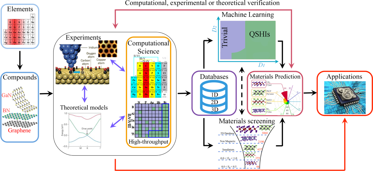
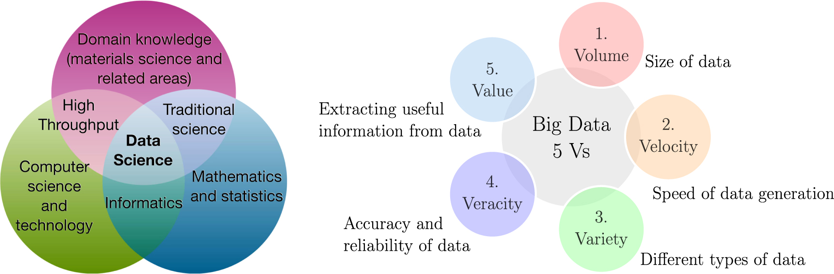
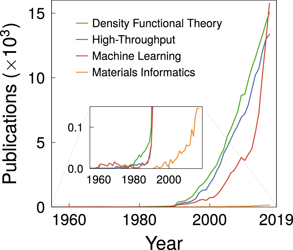
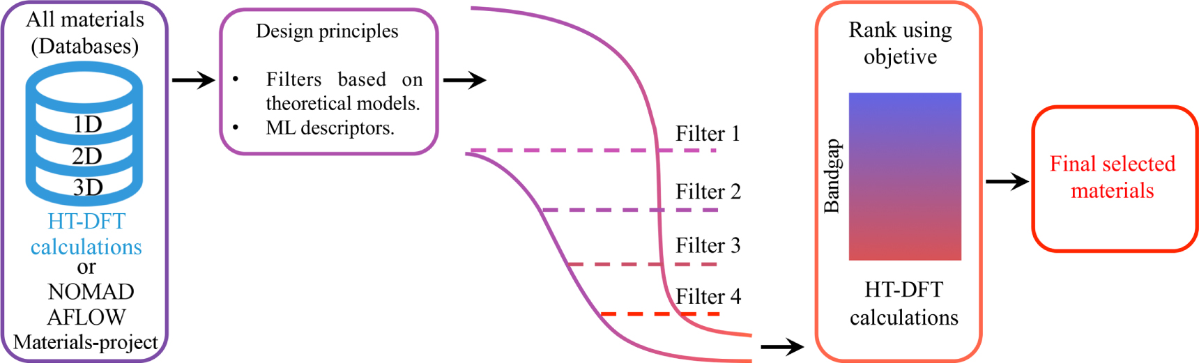
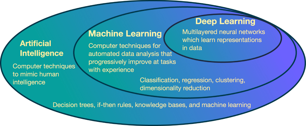
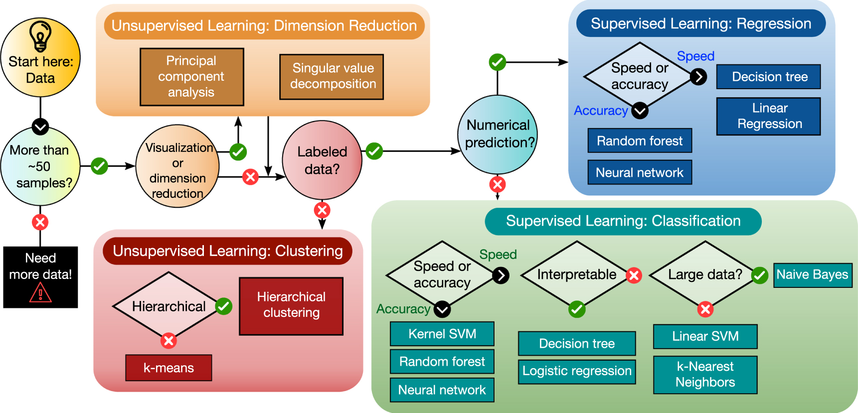
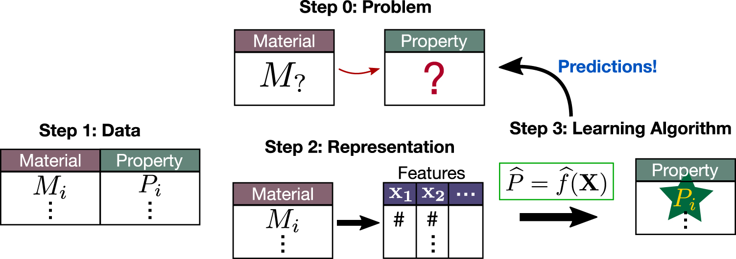
Figure 21. Materials maps for two- and three-dimensional compounds protected by the time reversal (TR) symmetry. For two-dimensional TIs (left), i.e., quantum spin Hall insulators (QSHIs), we show as an example the honeycomb functionalized compounds [2]. Left panel reproduced with permission from [2]. Here, there are materials whose topological class depends on functionalization (FD-QSHIs) and systems in which the topological character is independent of functionalization (FI-QSHIs). The descriptors D1 and D2 classifying tetradymite compounds (right) result in a convex-hull with very small superposition [506]. Right panel reproduced with permission from [506].
Download figure:
Standard image High-resolution image
3.2.5. Superconductivity
The discovery of a superconductor material dates back to 1911 and 46 years passed until the BCS theory managed to explain its properties. The first unconventional superconductor, or high-TC, was reported in 1975 and, despite enormous efforts from the scientific community, up to the present date, no theory has managed to contemplate the problem's full complexity. This lack of a comprehensive theory, capable not only of explaining but predicting novel superconductors, opens a wide road for modern computational science. Modern attempts used support vector regression to develop a regression model to estimate the TC of different superconductors of doped MgB2 [508]. More recently Stanev et al [509] presented the most comprehensive study of superconductivity using MI. The methodology combines data mining and ML with the random forest algorithm (see section 2.3.2) to investigate ≈16,400 superconductors harvested from the SuperCon experimental database [510]. They obtained the experimental chemical composition and TC from the database and compared the ML results using only elemental features, constructed using the Materials Agnostic Platform for Informatics and Exploration (Magpie) [203]. They obtained a regression model with  , which is notable given the different compositions of the dataset. With the regression model, 35 new non-cuprate and non-iron-based oxides have been identified as possible superconductors. The range of crystal symmetries is an interesting and non-induced surprise. They obtained 14 orthorhombic, 9 monoclinic, 6 hexagonal, 5 cubic, and 1 trigonal crystals. This path opens several possibilities for novel superconductors discoveries.
4. Conclusions and outlook
The data-driven era for materials discovery has been established by the Materials Genome Initiative, and the scientific community has just started embracing it. Electronic structure methods, led by density functional theory, and statistical learning methods, or simply machine learning algorithms, underwent great improvements over the last few decades. These are a consequence of the advances in computational capabilities, development of novel algorithms, and availability of data storage infrastructures. Their convergence represents a very fruitful and promising scenario for materials discovery. The major outcome of such convergence is the approximation between computational predictions and experimental realizations of novel materials. Therefore, the goal of reducing the time-to-market of new materials is starting to become a reality.
Successful applications exploring the above techniques have started to appear in the form of regression and classification models for prediction of basic properties, such as electronic band gaps, formation energies, and crystalline structures. The area of atomistic potentials have benefited early from machine learning methods, and as a consequence, this area shows relative maturity. Conversely, niches such as magnetic, superconductive, and other complex phenomena have just begun to be addressed. Nevertheless, they show great potential for further breakthroughs. Disentangling high-dimensional correlations is precisely where machine learning algorithms excel. Propelled by the recent creation of large databases, we also foresee an acute activity in the 2D materials and symmetry protected topological materials areas in the near future, regarding machine learning applications.
Lastly, the materials research field is shifting into a new paradigm of data-driven science. Relative success has been shown, nevertheless the construction of a broader route is an ongoing process. The possibilities and limitations are only starting to be grasped by the community, and the ever increasing amount of scientific data invites theoretical, computational and experimental scientists to explore it.
Acknowledgments
GRS, ACMP, CMA, MC, and AF acknowledge financial support from the Fundação de Amparo à Pesquisa do Estado de São Paulo (FAPESP), project numbers 2017/18139-6, 18/05565-0, 18/11856-7, 16/14011-2, 17/02317-2.