


Abstract
The Model-Analogs technique is used in the present study to assess the decadal sea surface temperature (SST) prediction skill over the Southern Ocean (SO). The Model-Analogs here is based on reanalysis products and model control simulations that have ∼1° ocean/ice (refined to 0.5° at high latitudes) components and 100 km atmosphere/land components. It is found that the model analog hindcasts show comparable skills with the initialized retrospective decadal hindcasts south of 50°S, with even higher skills over the Weddell Sea at longer lead years. The high SST skills primarily arise from the successful capture of SO deep convection states. This deep ocean memory and the associated decadal predictability are also clearly seen when we assess the Model-Analogs technique in a perfect model context. Within 30°S–50°S latitudinal band, the model analog hindcasts show low skills. When we include the externally forced signals estimated from the large ensemble simulations, the model analog hindcasts and initialized decadal hindcasts show identical skills. The Model-Analogs method therefore provides a great baseline for developing future decadal forecast systems. It is unclear whether such analog techniques would also be successful with models that explicitly resolve ocean mesoscale eddies or other small-scale processes. This area of research needs to be explored further.
Export citation and abstract BibTeX RIS

Original content from this work may be used under the terms of the Creative Commons Attribution 4.0 licence. Any further distribution of this work must maintain attribution to the author(s) and the title of the work, journal citation and DOI.
1. Introduction
The Southern Ocean (SO) plays a critical role in the global climate system mainly through its large influence on oceanic uptake of anthropogenic heat and carbon (e.g., Russell et al 2006, Marshall and Speer 2012). The deep SO can absorb and store heat/carbon and its efficiency is largely determined by the strength of meridional overturning circulation (MOC) (e.g., Sigman and Boyle 2000). Over the SO, the Antarctic bottom water (AABW) feeds the lower limb of the MOC. The AABW becomes the densest abyssal water as it moves down the continental slope and mixes with ambient water (e.g., Lumpkin and Speer 2007, Marshall and Speer 2012, Purkey and Johnson 2012, 2013). The return path of this deep water from the interior ocean to the surface is largely through SO upwelling that closes the MOC (Marshall and Speer 2012). Because of the long memory of deep ocean, the SO has been suggested to be one of the most predictable regions on decadal time scales (e.g., Boer 2004, 2011, Yang et al 2013, Zhang et al 2017a, b, Zhang et al 2019, Yang et al 2021, Zhang et al 2022b).
The decadal predictability is usually estimated by two common approaches: diagnostic and prognostic approaches. Boer (2004) estimated the sea surface temperature (SST) predictability over global oceans using a diagnostic predictability variance fraction (ppvf) method. The ppvf measures the ratio of slow potentially predictable component with respect to the total variance. The SO exhibits high values of ppvf and therefore has a large potential predictability. Zhang et al (2017a) then used a maximizing predictability method called average predictability time (APT, DelSole and Tippett 2009a, b) to examine the most predictable mode in a long control simulation from Geophysical Fluid Dynamics Laboratory (GFDL) CM2.1 model (Delworth et al 2006). They found that the most predictable SO SST mode is associated with the mature phase of SO internal deep convection variability. Using the same CM2.1 control simulation, Zhang et al (2017b) further estimate the SO perfect model predictability from a prognostic perspective, in which the control simulation at some time points is initialized by identical oceanic and perturbed atmospheric conditions. The spread within the ensemble is interpreted as an estimate of predictability. Again, they found that the SO decadal SST skill primarily arises from the deep ocean memory. Yang et al (2013) and (2021) extended this prognostic approach to the initialized real retrospective decadal forecasts/hindcasts. However, it is still very challenging on how to initialize the decadal prediction system and how to assess the prediction skill over the SO, largely because SO observations are very sparse in both time and space. This is in stark contrast to the North Atlantic and North Pacific Oceans where the observations are more numerous and can better be used for model initialization (e.g., Mochizuki et al 2010, Meehl and Teng 2012, Robson et al 2012, Yeager et al 2012, Yang et al 2013, Msadek et al 2014, Yeager et al 2018, Smith et al 2019, Smith et al 2020). Moreover, the initialized retrospective decadal forecasts require large computational resources and thus are only undertaken by large model centers.
Ding et al (2018) and (2019) proposed an alternative forecast method (Model-Analogs) to avoid additional forecast ensemble integration. In this method, the predictions are obtained from a long preindustrial control simulation by matching their selected variables to observed fields. The forecast members at various lead times are then taken from the subsequent evolution of these states in the control simulation. They showed skillful seasonal prediction of tropical Pacific SST anomalies using Model-Analogs. The skills in some regions such as the eastern equatorial Pacific even exceed that from initialized seasonal forecasts. In this study, we attempt to apply the Model-Analogs technique to decadal forecasts and try to evaluate if such a method is comparable to the initialized retrospective decadal hindcasts/forecasts over the SO. This Model-Analogs method may provide a benchmark for prediction skill when developing future decadal prediction systems.
2. Methods and models
In the Model-Analogs approach, we take advantage of large amounts of model output available from an existing long control simulation of a model. We refer to this data as a 'library' of climate states. For any observation, we then search through this 'library' for a small set of times where the model state most closely resembles the observed state by some metric. We then use the subsequent time evolution of these model states (which are closest to the observed state) as a forecast, with forecast spread corresponding to the differing time evolutions from these various selected time points in the control simulation. According to Ding et al (2018), the analogs we choose at each time t are through a distance metric ![$d\left(t,t^{\prime} \right)={\displaystyle {\sum }_{v=1}^{V}\displaystyle {\sum }_{j=1}^{J}\left[\tfrac{{T}_{j}^{v}\left(t\right)}{{\delta }_{T}^{v}}-\tfrac{{L}_{j}^{v}\left(t^{\prime} \right)}{{\delta }_{L}^{v}}\right]}^{2}$](https://content.cld.iop.org/journals/2515-7620/5/2/021002/revision2/ercacb90eieqn1.gif) by minimizing a distance between a target state T(t) and each library state L(t'). The target state is the observed state at the initialization time and the library state is from model's control simulation. The
by minimizing a distance between a target state T(t) and each library state L(t'). The target state is the observed state at the initialization time and the library state is from model's control simulation. The  denotes a variable and
  is the total number of variables. The j represents spatial grid points and J is the total number of grid points. The
  and
and  are the domain averaged standard deviation. To define analogs, we set V = 4 and constructed target and library states from SST anomalies (
 = 1), subsurface temperature anomalies at 1500 m depth (
 = 2), sea surface salinity (SSS) anomalies (
 = 3) and subsurface salinity anomalies at 1500 m depth (
 = 4) within the SO domain (50°S–77°S). We choose these four variables, because these variables control ocean stratification over the SO which is critical to the deep-water formation and thus determines the long memory of deep ocean. We then ranked the distance metric in an ascending order, and chose the P states closest to the target state as the model‐analog ensemble members
  where P is the analog index and
  is the time of this analog in the library. The subsequent evolution of ensemble within the control simulation
  is the Model‐Analogs forecast ensemble for T (t + τ) at lead time τ years.
The library dataset we used in the present study comes from the GFDL newly developed SPEAR (Seamless system for Prediction and EArth system Research) (Delworth et al 2020) simulation. We use SPEAR_LO version and its preindustrial control run has 4000 years. The SPEAR_LO has approximately 1° (refined to 0.5° at high latitudes) ocean and ice components from MOM6 (Adcroft et al 2019) and 100 km atmosphere and land components from AM4-LM4 (Zhao et al 2018a, b). The observations used for target states or the initial Model‐Analogs states are obtained from SPEAR_ECDA (Lu et al 2020) and SPEAR_atm_sst_restore reanalysis (discuss below). SPEAR_ECDA is based on SPEAR_LO and includes the ocean data assimilation (ODA) system in MOM6 as its backbone and incorporates the ocean tendency adjustment (OTA) bias correction scheme. SPEAR_ECDA assimilates a large amount of ocean observations such as the Argo dataset in recent years. We then average these two reanalysis datasets in their overlapping periods in to order to get a more reasonable 'observation'.
We compare the Model-Analogs based prediction skill with that from the retrospective decadal forecasts/hindcasts system initialized with SPEAR_atm_sst_restore reanalysis (Yang et al 2021). The SPEAR_atm_sst_restore is based on SPEAR_LO, in which the atmospheric winds and temperature were restored toward the 55-year Japanese Reanalysis (JRA-55) (Kobayashi et al 2015) and the SST was restored toward the NOAA Extended Reconstructed Sea Surface Temperature version 5 (ERSSTv5) data (Huang et al 2017). We then conducted a decadal retrospective forecast using the SPEAR_LO initialized from SPEAR_atm_sst_restore. The retrospective forecasts have 20 members and were initialized on 1 January every year from 1961 to 2021 and integrated for 10 years with the temporally varying historical forcings. To effectively remove the climate drift, the forecast anomalies for each variable were obtained by subtracting out the lead-time-dependent climatology from forecasts.
3. Perfect model predictability using model-analogs
We first assess the Model-Analogs technique in a perfect model context. In SPEAR_LO control simulation, we take the 1001–3500 years (abandon the first 1000-year data due to model spin-up process) as the library data and the last 500 years (3501–4000) is used for verification. The analog ensemble size (P) we set to 15. We test the sensitivity of perfect model skill on the ensemble size (P) and training data length and find the results are very similar when the ensemble size is larger than 10 and the library data is longer than 1500 years (Supplementary figure 1). We show in figure S2 (Supplementary figure) how well the model analogs reproduce the target states at zero lag. The correlation between the Model-Analogs ensemble means and target state is very high throughout the training region (white box in figure S2) for all four analogs (SST, SSS, subsurface temperature and salinity), suggesting high matches between the target states and model analogs. The highest matching regions are over the Ross, Amundsen-Bellingshausen and Weddell Seas. It is interesting to see the surface correlations (SST, SSS) are smaller than that in the subsurface variables (figures S2(a), (c) versus figures S2(b), (d)), which is probably due to smaller noises from the subsurface ocean. Overall, the model analogs capture the target states very well at zero lag within the training region. The correlation dramatically drops outside the training region.
We then show in figure 1 the perfect model skill of ensemble mean model-analog reconstruction of SO SST anomalies at different lead times. At a lead of 2-yr, the SST prediction skill is very high in most areas (figure 1(a)), with a maximum over the Ross and eastern Weddell Seas where the SST correlation exceeds 0.8. As the lead time increases, the SST correlation gradually decreases (figures 1(a)–(e)). At a lead of 10-yr, the SST correlation in most areas is still above 0.6 (figure 1(e)), indicating that the SO SST is predictable on decadal time scales. We note that the regions with high prediction skills (Ross and Weddell Seas) coincide with the SO deep convection regions in SPEAR_LO (Delworth et al 2020). This implies that the high SO SST skill is largely associated with the deep convection memory.

Figure 1. Perfect model skill (correlation) of Southern Ocean (SO) SST using Model-Analogs method at (a) 2-year lead, (b) 4-year lead, (c) 6-year lead, (d) 8-year lead and (e) 10-year lead. (f) Perfect model skill of SO area averaged (0°–360°E, 50°–70°S) SST skill as a function of lead years. (g) Perfect model skill of SO meridionally averaged (50°−70°S) SST skill as a function of lead years. The grey points overlapping on the shading denote that the SST correlation is significant at a 95% confidence level bast on a Student's t-test.
Download figure:
Standard image High-resolution imageWe further show in figure 1(f) the prediction skill of SO area averaged SST as a function of lead times. It confirms that the SO area averaged SST can be predicted 10 years in advance in this perfect model context. The longitude dependence of SST skill is clearly seen from figure 1(g). The SST correlation over the Ross (∼180°W) and Weddell (∼10°E) Seas shows the highest values and persists the longest. Again, this highlights the important role of SO deep convection in the SST prediction skill. To verify this speculation, we plot the SO SST and deep convection index (the AABW cell strength) in target states and those from model analogs at various lead years (figure 2). It is clearly seen that the model analogs well capture the SO deep convection evolutions (figure 2(b)). The convection persistence then provides a predictability source for the SO SST (figure 2(a)). These results are consistent with our conclusions from previous APT analysis and perfect model predictability experiments (Zhang et al 2017a, b). Thus, the Model-Analogs technique in essence successfully captures the most predictable mode over the SO in our model system.
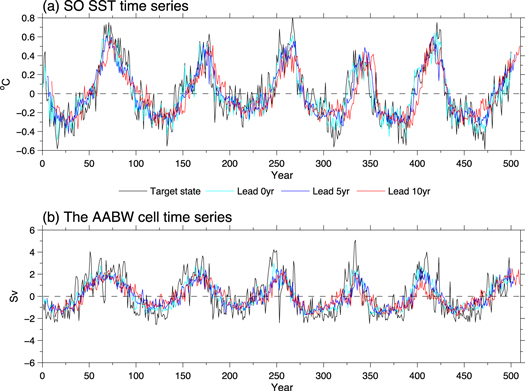
Figure 2. (a) SO area averaged (0°–360°E, 50°–70°S) SST anomalies (°C) from target state (2501–3000 year in SPEAR_LO control simulation, black line), 0-year lead (light blue line), 5-year lead (blue line) and 10-year lead (red line) Model-Analogs hindcasts in SPEAR_LO. (b) Same as (a) but for the Antarctic Bottom Water (AABW) cell index (Sv) time series. The AABW cell index is defined as the absolute value of minimum global meridional overturning circulation streamfunction south of 60°S, which well represents the SO deep convection strength (e.g., Zhang et al 2022).
Download figure:
Standard image High-resolution image4. Retrospective prediction using Model-Analogs versus using initialization
In this section, we use the Model-Analogs to make retrospective hindcasts of observed SST anomalies over the SO. To make real-world hindcasts using Model-Analogs, we choose the target state from 'observed' anomalies (SST, SSS, subsurface temperature and salinity) in years 1961–2021 and the data library from the entire dataset in SPEAR_LO control simulation (1001–4000 years). Since observations over the SO are very sparse in both time and space, particularly over the subsurface ocean, we use the averaged results of data assimilation product (SPEAR_ECDA) and SPEAR_atm_sst_restore reanalysis as a substitute for the observations. We construct model-analog hindcasts for forecast leads of 0–10 years. We set ensemble size P = 15 and there are only small improvements when the P further increases. We then compare ensemble mean model analog skills with the SPEAR retrospective decadal prediction system initialized with SPEAR_atm_sst_restore reanalysis (Yang et al 2021).
Figures 3(a)–(j) shows Model-Analogs and initialized decadal hindcast skills of observed SST anomalies at various lead times. The Model-Analogs overall show high prediction skills south of 50°S over the SO (figures 3(a)–(e)). The highest skill is mainly over the Ross, Amundsen, and Weddell Seas. The SST correlation gradually decreases as the lead time increases. The SST prediction skill over part of the SO can be predicted up to a decade (figure 3(e)). These SST skill characteristics using Model-Analogs share great similarities with that from perfect model (figures 1(a)–(e) versus figures 3(a)–(e)), suggesting that the predictability source may be the same in reanalysis and in model. The Model-Analogs also reproduce many details of skill from the initialized decadal hindcast (figures 3(a)–(e) versus figures 3(f)–(j)). Both sets of hindcasts are skillful over the Ross and Amundsen-Bellingshausen Seas, where SST correlation is as high as 0.7 even at a lead time of 10-yr. The initialized skills are generally comparable to that from Model-Analogs before 4-yr leads. After that, the Model-Analogs have higher skills over the Weddell Sea than the initialized hindcasts. Consistent with Yang et al (2021), the success of skill in initialized hindcasts mainly arises from the correct initialization of SO deep convection states, with strong AABW cell states around 1975–1985 and weak AABW cell states during 2000–2015 (figure 4(d)). The Model-Analogs technique also broadly captures the SO AABW cell evolutions in reanalysis (figure 4(c)). The long persistence of SO deep convection eventually reflects on the SST and provides a decadal predictability source for the SO SST skill (figures 4(a), (b)).

Figure 3. Model-Analogs hindcast skills of SO SST estimated by the SST correlation between ERSST and analog hindcasts at (a) 2-year lead, (b) 4-year lead, (c) 6-year lead, (d) 8-year lead and (e) 10-year lead. (f-j) Same as (a-e) but for the correlation between ERSST and decadal hindcast skills initialized from SPEAR_atm_sst_restore reanalysis. (k-o) Same as (a-e) but for the improved Model-Analogs hindcast skill by adding externally forced signals. The grey points overlapping on the shading denote that the correlation is significant at a 95% confidence level bast on a Student's t-test.
Download figure:
Standard image High-resolution image
Figure 4. (a) SO area averaged (0°–360°E, 50°–70°S) SST time series (°C) in ERSST (black line), Model-Analogs hindcasts at 0-year lead (light blue line), 5-year lead (blue line), and 10-year lead (red line). (b) Same as (a) but for the decadal hindcasts initialized from SPEAR_atm_sst_restore reanalysis. (c-d) Same as (a-b) but for the AABW cell evolutions. The black line denotes the AABW cell time series in reanalysis products (averaged value of SPEAR_ECDA and SPEAR_atm_sst_restore reanalysis).
Download figure:
Standard image High-resolution image
Figures 4(a) and (b) also display that the SO SST tends to warm in recent years. These warming anomalies are accompanied with an extreme low Antarctic Sea ice in late 2016 and persistent sea ice decreases thereafter (e.g., Wang et al 2019). The physical processes leading to these SO warming/sea ice decreases are primarily associated with the atmosphere forcings and upper ocean (0–500 m) variabilities (e.g., Meehl et al 2019, Zhang et al 2022b), which is very different from the warming around 1980s when the deep ocean process is involved. Thus, the ocean stratification (1500 m and 0 m) based Model-Analogs can't capture these upper ocean processes and thus have worse prediction skills than the initialized decadal hindcasts (figures 4(a), (b)).
It is also worth noting that the SST prediction skill north of 50°S in the initialized hindcasts is much higher than that from Model-Analogs (figures 3(a)–(e) versus figures 3(f)–(j)). Within 30°S–50°S, the SST shows a strong warming trend in both observation and climate models (Armour et al 2016). This warming trend is largely associated with the greenhouse gas induced warming and is thus driven by external forcings (e.g., Marshall et al 2015, Armour et al 2016, Liu et al 2018). The physical processes are as follows: the heat uptake mainly occurs south of 50°S in the SO. This heat is then balanced by an anomalous northward heat transport by the mean Deacon Cell. The heat is eventually converged within the 30°−50°S latitudinal band. Since the Model-Analogs are constructed from a pre-industrial control simulation, the externally forced signals are not taken into consideration. According to Ding et al (2019), we improve this disadvantage of Model-Analogs by using the ensemble mean of SPEAR_LO large ensemble (LE) simulations (Delworth et al 2020) to estimate the externally forced signals (see supplementary information). Prior to searching for model-analogs in a long control simulation, we remove the externally forced signal from the reanalysis products. The predicted forced trend component from LE simulations is then added back to the final hindcasts. Figures 3(k)–(o) show the SST prediction skills at various lead times after adding the externally forced component. Apparently, including the external radiative forcings largely improves the SST prediction skill of the Model‐Analogs hindcasts within 30°S–50°S.
5. Discussion and summary
In the present study, we use Model-Analogs method to assess the decadal SST prediction skill over the SO. South of 50°S, the model analog hindcasts (constructed from observation-constrained reanalysis and SPEAR_LO control simulation) show comparable skills with the initialized retrospective decadal hindcasts. As the lead time becomes longer, the SST skill over the Weddell Sea using Model-Analogs is even higher. The high SST skill in both hindcasts primarily arises from the successful capture of SO deep convection states. This deep ocean memory and the associated decadal predictability are also clearly seen from the perfect model context using Model-Analogs. Within 30°S–50°S latitudinal band, the model analog hindcasts show low skill due to the absence of external forcing. When we include the externally forced secular trend estimated from LE simulations, the model analog hindcasts and initialized decadal hindcasts show identical skills. These results are very exciting, since we can make forecasts only based on observation constrained reanalysis and model control simulation, without running expensive assimilation initialized prediction model. The Model-Analogs method therefore provides a baseline for prediction skills when developing future decadal forecast systems.
The decadal predictability source of SO SST in SPEAR model and reanalysis is largely associated with the SO deep convection (or the AABW cell) states. Due to sparse SO observations in both space and time, it is difficult to evaluate the exact strength and variability of this AABW cell. Purkey and Johnson (2012) and (2013) suggested a global-scale slowdown of the AABW cell during 1979–2012 in observation. It seems that this weakening trend is consistent with what we have seen in SPEAR reanalysis. It is also not clear if the SO deep convection oscillates in the real world. Some studies suggested the SO low-frequency variability has likely occurred in the past climate (e.g., Cook et al 2000, Le Quesne et al 2009) but is not sure if it exists in the current and future climates (Zhang et al 2022a). The SPEAR_LO is a 'convecting' model, which offer a glimpse into the potential decadal predictability over the SO in the presence of low-frequency convection variability. Zhang et al 2021 suggested that the SPEAR_LO may overestimate the amplitude of low frequency convection variability relative to observations. Here, we also take a control simulation from SPEAR_MED that has a weaker convection variability compared to SPEAR_LO (Zhang et al 2022a) as library data to search for analogs. We find the SST prediction skill over the SO indeed decreases due to a weaker persistence of convection in SPEAR_MED (figures S3, 4). Thus, it remains unclear to what extent the SO convection variability can imprint on the SST predictability in the real world. Note also that we choose reanalysis products as our initial Model‐Analogs states. These reanalysis datasets come from the same model family and resolution of our decadal hindcasts, and therefore biases are likely to be common between our model-analogs and these systems, although SPEAR_ECDA reanalysis employed the bias correction scheme. It is important to apply the Model-Analogs technique to other models, reanalysis products and compare them with the initialized decadal hindcasts from different model centers in the future.
As mentioned in the methods section, we chose four variables including both surface and subsurface ocean variables to define analogs. Because these variables control ocean stratification over the SO which is critical to the deep-water formation and thus determines the long memory of deep ocean. When we only use SST to define analog or add atmosphere variable (e.g., low frequency sea level pressure), the SO SST skill using Model-Analogs technique largely decreases and is worse than the initialized hindcasts (Supplementary figure S5). This suggests that the subsurface ocean is a necessary condition for the high decadal prediction skill over the SO.
Thus, we also call for improved and sustained measurements of the SO, particularly over the subsurface ocean, using new technologies, which could produce better target states for Model-Analogs and better initialization for future prediction system.
Acknowledgments
We thank Sonya Legg and Tony Rosati for their extremely valuable suggestions and comments on our paper as GFDL internal reviewers. The work of T.L.D, X.Y and F.Z is supported as a base activity of NOAA's Geophysical Fluid Dynamics Laboratory. L.Z, F.L and Y.M are supported through UCAR or Princeton University under block funding from NOAA/GFDL or JAMSTEC.
Data availability statement
The data that support the findings of this study are openly available at the following URL/DOI: 10.5281/zenodo.7562575.
Data and code availability
The Japanese 55-year Reanalysis JRA-55 is available at https://jra.kishou.go.jp/JRA-55/index_en.html. The ERSSTv5 is available at https://www.ncei.noaa.gov/products/extended-reconstructed-sst. The data for figures are available online at https://zenodo.org/record/7562575#.Y87b9S1h1pQ. The source code of ocean component MOM6 of SPEAR_LO model is available at https://github.com/NOAA-GFDL/MOM6.
Competing interests
The authors declare no competing interests.
Supplementary data (3.3 MB DOCX)