

Abstract
A study was conducted in Thuma area in central Malawi to quantify contemporary land cover and to explore the degree of land use change in the Thuma forest reserve area of Malawi by analysing and comparing satellite-derived land cover maps from 1997, 2007 and 2017. The study was carried out using Remote Sensing and Geographic Information System (GIS), focusing on analysis of Landsat 5 ETM and Landsat 8 ORI/TIRS satellite images. The classification was conducted for the following distinct classes; closed forest, open forest, shrubland, savanna grassland, agriculture fields, and water. The analysis revealed that closed forest diminished from 19% in 1997 to 10% in 2007 to 6% in 2017. Open forest reduced from 30% to 21% from 1997 to 2007 but increased to 22% in 2017. Agriculture area almost doubled from 37% in 1997 to 64% in 2017. The actual area from 1997 to 2017, shows that closed forest has reduced from 7,000 ha to 3,000 ha while open forest from 12,900 ha to 7800 ha. Savanna grassland has doubled from 5,900 ha to 13,000 ha. However, future studies should use modern satellites such as Sentinel and Landsat 9 for improved quantification of changes. The findings show that even the protected forest reserve (previously dominated by closed forest) is not fully protected from deforestation by local communities. Government and other stakeholders should devise measures to meet the needs of the surrounding communities and the ecological/biophysical needs of the reserves. Based on this study, issues of re-demarcation of the forest reserve and the accessed area should also be explored. This study serves as a reference for the management of Thuma Forest Reserve as a refuge for natural tree species, rivers that harbour endemic fish species (Opsaridium microlepis and Opsaridium microcephalis) and the sustainable management of endangered elephants in the reserve.
Export citation and abstract BibTeX RIS

Original content from this work may be used under the terms of the Creative Commons Attribution 4.0 licence. Any further distribution of this work must maintain attribution to the author(s) and the title of the work, journal citation and DOI.
1. Introduction
Land cover and land use mapping have become crucial components in the assessment and management of natural resources. Assessment of land cover dynamics is an essential requirement for the sustainable management of the environment and represents a fundamental baseline through which to support activities linked to environmental studies (Tiwari and Khanduri 2011). An accurate and updated land cover database is multipurpose in its utility and can support the assessment of landscape dynamics. This can be used to facilitate the planning of environmental restoration activities (Latham 2013).
Most protected forest reserves have failed to meet the expectation of increasing forest cover due to anthropogenic interferences (Kusimi 2015). Detection of land cover changes as a result of land use modification especially those changes caused by humans is paramount in policy decision making for sustainable management of natural resources (Estoque and Murayama 2015). Current studies in most sub-Saharan countries show that there is a general reduction in forest cover in most protected forest reserves due to expansion of agricultural land or mere tree removal for other amenities (Damnyag et al 2013, Kayombo et al 2020, Skole et al 2021, Appiah et al 2021). In East and parts of southern Africa, land use changes from natural forests/woodlands/grasslands to agriculture with clear ecosystem regime shifts (Bullock et al 2021).
Malawi is endowed with a wide range of natural resources that can support sustainable socio-economic development. The main land cover types in Malawi are agriculture, forest, herbaceous plants, forest plantations, shrubs, built-up areas and water bodies (Munthali et al 2019). These resources are under constant modification due to direct and indirect factors such as population growth, poverty, deforestation, uncontrolled fires and lack of environmental awareness resulting in increased degradation of the environment, with significant loss of soil fertility, soil erosion, siltation, pollution and loss of biodiversity (Environmental Affairs Department 2010). From 1999 to 2018 the country lost woodlands from 4.4 million ha to 3.4 million ha (Gondwe et al (2020)). The greatest shift was from forest area to agriculture and settlement. With the increasing rate of population growth (2.8%) and a current population of 17.5 million (National Statistics Office 2018), the pressure on forest resources is expected to increase. For example from 1990 to 2010, the area under agriculture fields increased from 42,560 km2 to 47,040 km2 representing a 9% increase in central east of Malawi (Latham 2013). There is high demand for general forest related products for indigenous trees, shrubs to support high domestic energy needs especially the need for firewood and charcoal (Environmental Affairs Department 2017) for cooking and burning of bricks.
Special interest for a study in Thuma area, Central Malawi is motivated by the vastness of the reserve and the attention it has received from government and other partners on natural resources management. The reserve is considered a refuge for tree diversity and elephant management (Worldlife Action Group (2018)). Apart from the native animals, the reserve is home to about 200 elephants which were transferred from other 'non-safe' reserves of the country for safety. The reserve also harbours part of Linthipe River which is a breeding niche for Opsaridium microlepis and Opsaridium microcephalis fish species (Salima (2019)). The reserve has also undergone a number of management reforms from government to non-governmental organization (NGO) with the aim of achieving forest management and animal population (Government of Malawi 1996). However, Thuma Forest Reserve area faces considerable pressure for its forest resources from the surrounding communities and Lilongwe city (Environmental Affairs Department 2017). Temporal assessments to establish land use and land cover changes are essential in answering the questions associated with land cover and land use changes to the physical and social environments (Munthali and Murayama 2011, Kpienbaareh and Oduro Appiah 2019, Appiah et al 2021). The land cover maps and analysis of the changes will be the basis for the sustainable management of the Thuma reserve. The national land cover and land use changes have been tried but have been marred by financial, capacity and technical hiccups (Orlovsky et al 2006, Environmental Affairs Department 2017). It is not directly easy to assess land cover and land use changes over huge areas especially when conventional methods are used. Locally-based land use and land cover change assessments help capture or quantify changes with an increased level of accuracy. Spatial and temporal scale changes in vegetation cover or productivity indicate probable impending desertification and or degradation processes in an area. It is, therefore, imperative that area-specific assessments be encouraged because the ecological/landscape changes on land use/land cover are more evident at local than national level (Collado et al 2002). These assessments help gauge the level of vegetation loss, impending ecological threats, or extent of success of afforestation interventions in previously bare areas. This information will help in policy decision-making and identification of land use changes that have effects on the land cover of the reserve. Sound decisions based on knowledge in the dynamics of land cover and land use changes of the area will contribute in attaining the United Nations Sustainable Goals 13 and 15. Goal 13 seeks appropriate actions that contribute to climate change mitigation while Goal 15 seeks to achieve sustainable management of land-based resources by preventing desertification, restoring and protecting the terrestrial resources by 2030 (United Nations (2016)). Therefore, the objective of this study was to quantify contemporary land cover and to explore the degree of land use change in the Thuma forest reserve area of Malawi. This was accomplished by analysing and comparing satellite-derived land cover maps from 1997, 2007 and 2017. The assessment responded to a research question 'What is the degree of change in the selected land use classes (closed forest, open forest, shrubland, savanna grassland, agriculture fields, and water) from 1997, 2007 and 2017 in the Thuma forest reserve area?'
2. Methodology
2.1. Study area
Thuma area lies on the borders of Salima, Dowa, Lilongwe and Dedza districts (13.78° South latitude; 34.43° East longitude), central region of Malawi (figure 1). It is approximately 80 km from the capital city (Lilongwe) by road. The area covers approximately 42, 437 ha and it sits on an elevation of between 557 to 1,564 m above sea level of which, 19,700 ha comprise a protected forest reserve called Thuma Forest Reserve (Worldlife Action Group (2018)). Generally, the topography is rugged. The lower parts of the area are covered by savanna grasslands with patches of clearing for agriculture while the upper rugged levels are covered in Brachystegia (Miombo) woodland (Worldlife Action Group 2018, Nyirenda et al 2019). The area was physically delineated to include Thuma Forest Reserve and its surrounding area based on the hydrology network of the area, especially focusing on the small tributaries around the forest (figure 1). This area supports livelihoods in Salima, Dowa, Lilongwe and Dedza districts. It is a source of several small rivers, source of energy (firewood and charcoal), habitat for a range of flora and fauna, including elephants. Communities around Thuma area practice subsistence and commercial agriculture systems. Those involved in subsistence mainly grow maize, groundnuts, beans and vegetables while those practicing commercial agriculture grow tobacco which requires firewood for curing (Crops Department Report 2017).
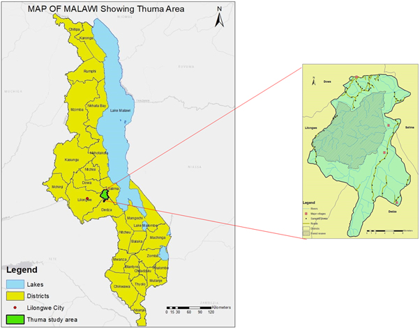
Figure 1. Map of Malawi showing Thuma study site and district boundaries.
Download figure:
Standard image High-resolution image2.2. Work flow
The procedure, as shown in figure 2, involved imagery acquisition, pre-processing to remove atmospheric errors, to get a clear view of the satellite images, enhancement and interpretation of the images. Field validation was done at the study site to obtain photos and descriptions of the sampled points. Unsupervised and supervised classification were performed on the images based on ground truth data. Error assessment was done to determine the level of accuracy of the classification exercise and finally, imagery change detection was performed.
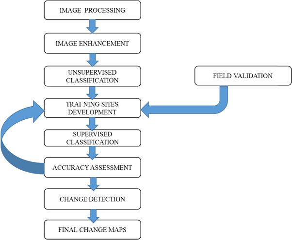
Figure 2. The summarised workflow for land cover change detection procedure.
Download figure:
Standard image High-resolution image2.3. Data sourcing
2.3.1. Satellite images used
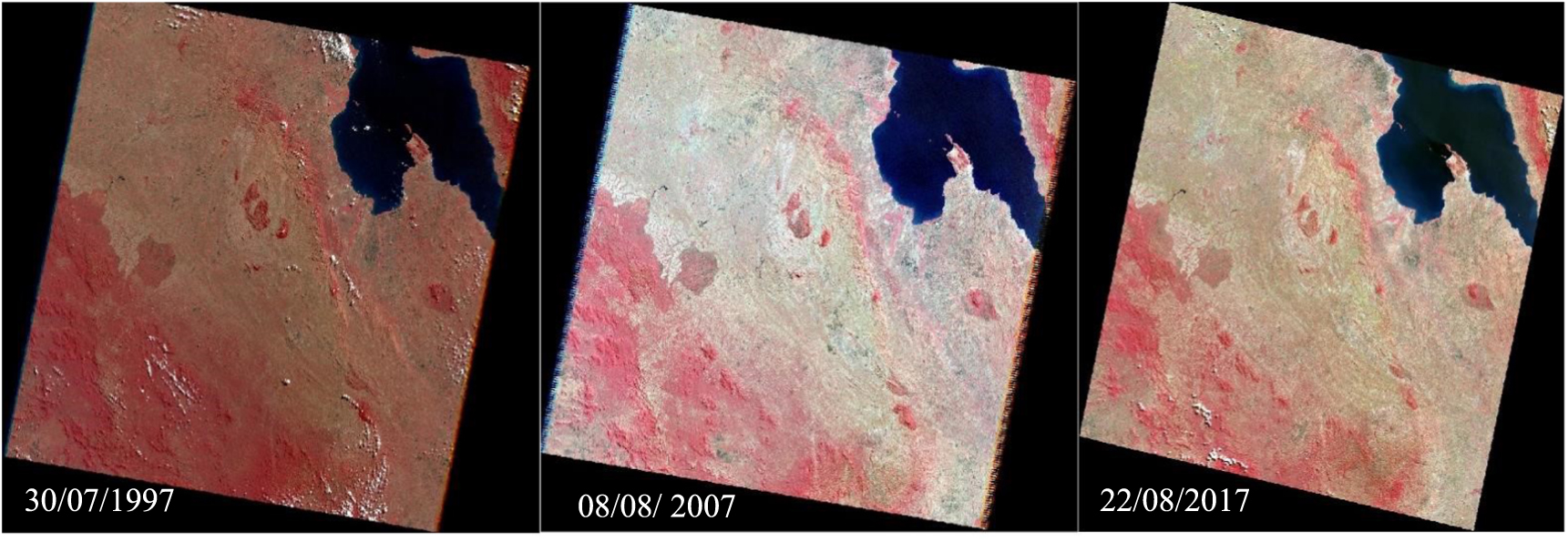
Landsat imagery data (figure 3) was used for land cover classification because it is free, has a long history (since 1972 to date) and higher frequency of archives with an average temporal resolution of 16 days (Manandhar et al 2009). For the year 1997 and 2007, Landsat images from Landsat 5 Thematic Mapper were used, which was operational from 1984 to 2013. Landsat 5 was used because Landsat 7 went into permanent malfunctioning on 31 May 2003 due to a fault in the satellite's Scan Line Corrector (SLC) (United States Geological Survey online 2021). For 2017, Landsat 8 Operational Land Imager and Thermal Infrared Sensor were used. Landsat 8 has more bands than Landsat 5 because it carries two sensors. It has additional band 1, deep blue visible channel for viewing water and coastal areas and band 9 for detection of Cirrus clouds (Mwaniki et al 2015). The images were downloaded from the United States Geological Survey website (GloVis). We specified the time of the imagery concentration on summer months because that is the time to obtain clear images for Malawi (Gumma et al 2019). Cloud cover was specified from 0 to 10%.

Figure 3. Landsat Images for Thuma area, path 168, and row 70, for the years 1997, 2007 and 2017. Reproduced from United States Geological Surveys website. Images stated to be in the public domain.
Download figure:
Standard image High-resolution imageFor this image analysis, seven bands from Landsat 5 and Landsat 8 were used. Band 1 (Blue green) differentiates soil and rock surfaces from vegetation. Band 2 (Green) covers the green reflectance peak from leaf surfaces near the visible spectrum (Lillesand et al 2015). Band 3, is the red band chlorophyll absorption band which helps in distinguishing vegetation and monitoring vegetation health. In this study, it was useful in distinguishing between closed forest, open forest, shrubland and grassland. The Near Infra-Red (NIR) Band 4 is good for differentiating vegetation, soil and water. To view false colour in Landsat 5, a combination of bands 4,3,2 was used. This means that to view vegetation, band 4 (NIR) was used basing on its wavelength which has high reflectance at 0.7 to 0.9 micrometres. In Landsat 8, band 5 (NIR) which ranges from 0.851 to 0.879 micrometres (figure 5) was used to view vegetation. Different types of vegetation possess different types of spectral signatures. Bands 5,4,3 were used to view false colour in Landsat 8. Vegetation is viewed in red in false colour because green and blue are absorbed and only red is reflected by vegetation. Vegetation has a unique spectral signature which enables it to be distinguished readily from other types of land cover in the near-infrared. So, in vegetation mapping, this was mainly used to distinguish between closed forest, open forest and shrubland, agriculture and savanna. Water absorbs all colours, so the rivers were appearing as dark blue.
2.3.2. Field validation
Field validation process is done to improve the quality and accuracy of the data base (Latham 2013). In this study, field validation was done to obtain ground truth data to be used in image training for classification. Ground truth points were sampled from a polygon of the study area. The validation samples were collected for the year 2017. The samples were randomly selected in a Stratified Random Sampling based on accessibility (along the roads/paths) of the study area and location homogeneity (Gumma et al 2019). They were generated in ArcMap and were converted to GPX format and uploaded in a Geographic Positioning System (GPS) device which was then used to locate the sampled points on the ground. A total of 60 points (See appendix A) were selected. A deliberate effort was made to sample areas where it was difficult to distinguish the land cover classes in the preliminary interpretation, especially between savanna grassland and agriculture fields or open forest and shrubland. Four photographs, in the directions of North, East, South and West were taken at each point and dominant land cover was recorded (Manandhar et al 2009). Some examples of the selected points are shown in table 1.
Table 1. Some of the validated points in the study area (more points are shown in appendix A).
| Point | Easting | Northing |
|---|---|---|
| 0 | 637080 | 8479544 |
| 1 | 636826 | 8478643 |
| 2 | 630827 | 8478621 |
| 3 | 629765 | 8477006 |
| 4 | 636110 | 8478851 |
| 5 | 631961 | 8478261 |
| 6 | 635164 | 8476936 |
| 7 | 631819 | 8474283 |
| 8 | 631519 | 8472852 |
| 9 | 634957 | 8479174 |
| 10 | 640823 | 8474648 |
| 11 | 624760 | 8468006 |
| 12 | 622728 | 8464608 |
| 13 | 640846 | 8453449 |
| 14 | 641284 | 8454046 |
| 15 | 641837 | 8454484 |
2.4. Image pre-processing
2.4.1. Atmospheric correction
Atmospheric correction was done to influence the pixel values of the image in order to adjust the values to compensate for the atmospheric effect (Campbell and Wyne 2011). The energy that is captured by Landsat sensors is influenced by the Earth's atmosphere. These effects include scattering and absorption due to interactions of the electromagnetic radiation with atmospheric particle like aerosols, gases and water vapour. Hence the need to correct the atmospheric Landsat data to earth surface values (Young et al 2017). Atmospheric correction was done for only Landsat 5 data in Quantum GIS, using the SCAP plug in. The correction was done in all the seven bands (Sharmila 2013). There was no need to perform atmospheric correction for Landsat 8 data because its data already have in-built atmospheric corrections. At-satellite radiance was calculated from Digital Number (DN) values basing on the maximal and minimal spectral radiance value (or the gain and bias) for each band (Chander et al 2009). The following equation was used for atmospheric correction (Cui et al 2014).

Atmospheric correction, Where Lβsat = Spectral radiance at the sensor, DNcal = Digital numbers from a specific band, Gainβ = Radiometric gain and Biasβ = Radiometric bias
2.4.2. Cloud removal and masking
The 1997 Landsat 5 satellite image had clouds in southwest area. So, ArcMap spatial analyst tool was used to remove the clouds. An equal area was clipped out of all three images. Since forests are characterized by dark colour due to chlorophyll and shadows they cast in the visible band realm (Goward et al (1994); Huemmrich and Goward 1997), they are easily distinguished in image processing (Dodge and Bryant 1976). This forms the basis for setting boundaries for delineation of pixel for true colour representation in Landsat images. Pixel area delineation was done using histogram in the local image window. Due to their darker nature of forest images, they appeared at the base of the histogram. Cloud delineation was done by normalizing the temperature at each isometric zone. The details of this procedure are provided by Huang et al (2010). Then linear cloud boundaries were made to achieve non-infrared bands in the Landsat image to construct the spectral-temperature space. The shadows of the clouds were detected spectrally and geometrically. Each cloud pixel was detected with reference to location, solar illumination and cloud height. An appropriate lapse rate was used to estimate cloud height (Smithson et al 2008). Finally, a determination of a classification was made.
2.5. Image processing
2.5.1. Image enhancement
The images were imported and opened in ArcMap where all the bands from 1 to 7 were stacked using the composite band tool. Image enhancement was performed on the images to improve visibility. In ArcMap the Dynamic Range Adjustment tool together with the stretched and red green and blue (RGB) composite tools were employed (Jia and Richards 2006). False colour image combination was used because it fits well with the target of viewing forest and other vegetated land covers. Because of the spectral signature of vegetation (Appendix B), the classes were distinguished visually using Near Infrared, Red and Green bands. Summarily, all the desired rigorous protocols/procedures were followed to identify the respective classes using the high-resolution images from Google Earth for the large volumes of data. The technique termed, Spectral Matching Technique has been fully described and used by Thenkabail et al (2007), Gumma et al (2011), Gumma et al (2016).
2.5.2. Unsupervised classification
Unsupervised classification was performed on the images so that land cover classes with similar spectral signatures could be easily identified. This process was run on a seven-band stack of all the images to gauge the performance of the software on the classification of the pixels depending on the specified number of classes without human intervention. This process helped getting a general understanding of the probable land cover classes in the area to be input as training sites in supervised classification (Liu et al 2003). The IsoCluster unsupervised method was used in ArcMap for computing the minimum Euclidean distance when assigning each candidate cell to a cluster using a modified iterative optimization clustering procedure, also called Migrating Means Technique. The algorithm separated all the cells into the user-specified number of distinct unimodal groups in the multidimensional space of the input bands (Lillesand et al 2015). The result from the unsupervised classification was nine distinct classes of which only two (water and closed forest) could relate to the situation on the ground.
2.5.3. Supervised classification
Supervised classification was conducted in order to extract quantitative information from remotely sensed Landsat images data. The goal of supervised classification was to assign each pixel in a study area to a class or category. In this classification, knowledge about the study area was obtained from field validation which was used to identify representative areas, or samples of each class (Feringa et al 2001). The training sites were determined by ground truth data, an average of twenty training areas were done per class. The training areas were larger for big classes like agriculture and small for small classes like shrubland and water. The classification was based on the following distinct land cover classes; closed forest, open forest, shrubland, savanna grassland, agriculture fields and water. In the present study, training sites for these classes were developed and run to classify the images of interest. A classification signature file was created for 2017 image which was then used as the basis for classifying 2007 and 1997 images. This was then used to run the maximum likelihood classification in ArcMap. The resulting product was a classified raster image with the five land cover classes for each year. The symbols and colours of the classes were edited and labelled appropriately. After observing the results of the accuracy assessment, training samples or classification parameters were adjusted to get a better result or more accurate classification (Herold et al 2008).
2.6. Error assessment
Accuracy assessment was done to compare a classified image with the ground truth data to assess the reliability of the data (Congalton 1991). Classification error occurs when a raster pixel belonging to one land cover class is assigned to a different land cover class. Errors of omission occur when a feature is not included in the category being evaluated; errors of commission occur when a feature is incorrectly added in the category being evaluated. An error of commission in one category will be counted as an error in omission in another category (Feringa et al 2001). An error matrix compares the relationship between known reference data and the results of the classification, based on the classes. In this study, accuracy assessment was done for the 2017 classified raster image. A total of 180 points were randomly selected from the polygon of the study area using the sampling tool in ArcMap. This point layer was used to extract values from the classified 2017 raster. The random point layer was converted to Keyhole Markup Language (KML) format and exported and opened in Google Earth Pro. In Google Earth, an image dated close to June 2017 was used. Google Earth image was used for classification because the ground truth data from sixty points were not adequate to use in error assessment. Observations were made and recorded as to what type of land cover the points were falling on. This information was transferred to the extracted values attribute table where they were entered in a field. The attribute table of this layer was used to create fields for running frequency using the frequency statistics tool in ArcMap. After obtaining the frequency table, pivot table statistical tool was used to pivot the frequency table into an error matrix table. Calculations were done in the confusion matrix and it was established that the classification had an accuracy of 68%.
2.7. Change detection analysis
After developing a classified land cover map for each year in ArcMap, the Spatial Analyst Zonal Statistics Tool for cross tabulating areas was used to detect changes in land cover per class. The tool detects the exact area change (land use) on the 30 m by 30 m pixel size. This was run for the six classes from a 1997 land cover class to a corresponding class in 2007. Then a cross tabulation was done for the area change for a class in 2007 to 2017. The results came as statistical tables showing changes per class per year (ArcGIS User Manual 2018). These results were also presented as percentage changes per class per year. During field validation, only 60 points were sampled due to logistical hiccups and inaccessibility of some sites, but the ideal would be more than 50 points per land cover class (Congalton 1991). However, Google Earth image was used to validate inaccessible points to minimize errors. Finally, a land cover change study interval of 10 years was used. The confusion matrix was done for 2017 only because it was possible to compare the ground truth and classified land cover unlike the cases for 1997 and 2007. The accuracy result from the confusion matrix was 68% representing the moderate agreement between the reference data and the classified image (Jensen 2004).
3. Results
Premised on the purpose of this study, land cover classification for the study area was run for 1997, 2007 and 2017. The results are presented in form of maps, charts and tables. The overall land cover changes are shown in figures 6 and 7. Tables 2–5 show a detailed percentage change in ha of land cover from one class to another between the years.
Table 2. Land Cover change between time intervals in percentages from original class in Thuma area, central Malawi. (The rows are changes in percentage from a 1997 class to a 2007 class. For example, 28.1% of land which belonged to closed forest class in 1997 changed into open forest class in 2007). Role with totals indicate hectares per cover class.
| 1997 to 2007 | Closed forest | Savanna grassland | Agriculture | Open forest | Shrubland | Water | Total 1997 |
|---|---|---|---|---|---|---|---|
| Closed forest | 48 | 6.4 | 11.1 | 28.1 | 6.3 | 0.1 | 100 |
| Savanna Grassland | 0.4 | 40.5 | 12.4 | 9.6 | 36.8 | 0.3 | 100 |
| Agriculture | 0.3 | 30.9 | 47.6 | 10.2 | 10.5 | 0.6 | 100 |
| Open forest | 4.6 | 18.9 | 16.4 | 40.1 | 19.1 | 0.8 | 100 |
| Shrubland | 0 | 72.8 | 8.3 | 3.7 | 14.5 | 0.8 | 100 |
| Water | 0.9 | 37.1 | 11.7 | 4.8 | 3.7 | 41.8 | 100 |
| Total | 4395.6 | 12,485.88 | 8,925.93 | 8.994.42 | 6,790.32 | 353.34 |
After the image analysis process and classification, the distinct land cover classes that could be clearly differentiated from the 30 m resolution Landsat images were; Closed Forest, Open Forest, shrubland, Savanna Grassland, Agriculture and Water. As it can be observed from the maps and graphs (figures 4–5), it is evident that generally closed forest area is dwindling from 19 percent in 1997 to 11 percent in 2007 to 6% in 2017. Savanna grassland increased from 13 percent in 1997 to 30 percent in 2007 to 31% in 2017. The dominant land cover classes in 2007 and 2017 are agriculture and savanna grasslands. Only two rivers of Linthipe and Linduzi (water bodies) were visible on the 30 m × 30 m imagery. Arear under water decreased by over 50%.
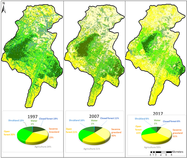
Figure 4. Land cover change maps and the percentage changes, Thuma forest area of central Malawi, Africa.
Download figure:
Standard image High-resolution image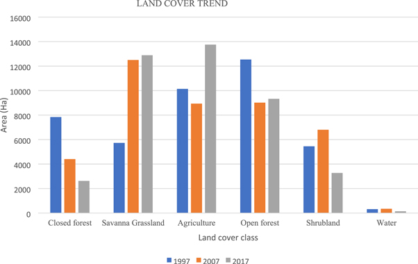
Figure 5. A graph showing land cover change in area (hectares) per class for the different years, Thuma forest reserve area, Malawi, Africa.
Download figure:
Standard image High-resolution imageTable 3. Land Cover change between time intervals in percentages from original class in Thuma area, central Malawi. (The rows are changes in percentage from a 2007 class to a 2017 class. For example, 30.45% of land which belonged to savanna grassland in 2007 became agriculture in 2017). Role with totals indicate hectares per cover class.
| 2007 to 2017 | Closed forest | Savanna grassland | Agriculture | Open forest | Shrubland | Water | Total 2007 |
|---|---|---|---|---|---|---|---|
| Closed forest | 44.64 | 6.75 | 10.76 | 35.49 | 2.35 | 0.01 | 100 |
| Savanna Grassland | 0.12 | 54.73 | 30.45 | 6.89 | 7.61 | 0.20 | 100 |
| Agriculture | 0.35 | 19.81 | 60.07 | 15.03 | 4.62 | 0.12 | 100 |
| Open forest | 5.99 | 17.60 | 23.70 | 45.30 | 7.37 | 0.05 | 100 |
| Shrubland | 0.93 | 34.50 | 26.66 | 20.97 | 16.88 | 0.06 | 100 |
| Water | 0.00 | 10.47 | 46.68 | 15.18 | 0.74 | 26.94 | 100 |
| Total | 2,610.9 | 12,853.53 | 13,730.76 | 9,312.3 | 3,275.1 | 139.95 |
Table 4. Land cover change between time intervals in percentage to new class (The rows are changes in percentage to a 2007 class from 1997 class. For example, 25.1% of land which belonged to agriculture class in 2007, came from savanna grassland in 1997). Role with totals indicate hectares per cover class.
| 1997 to 2007 | Closed forest | Savanna grassland | Agriculture | Open forest | Shrubland | Water | Closed forest |
|---|---|---|---|---|---|---|---|
| Closed forest Savanna | 85.5 | 4.0 | 9.7 | 24.5 | 7.3 | 2.8 | 18.7 |
| Grassland | 0.5 | 17.7 | 7.6 | 5.8 | 29.5 | 3.9 | 13.0 |
| Agriculture | 0.7 | 25.1 | 53.9 | 11.4 | 15.6 | 15.9 | 24.1 |
| Open forest | 13.1 | 19.0 | 23.1 | 55.8 | 35.3 | 28.1 | 29.9 |
| Shrubland | 0.0 | 33.4 | 5.3 | 2.3 | 12.2 | 12.7 | 13.6 |
| Water | 0.1 | 0.9 | |||||
| Total | 4,395.6 | 12,485.88 | 8,925.93 | 8.994.42 | 6,790.32 | 353.34 |
Table 5. Land cover change between time intervals in percentage to new class in Thuma central Malawi (The rows are changes in percentage to a 2017 class from 2007 class. For example, 15.28% of land which belonged to shrubland in 2017 came from open forest in 2007), Role with totals indicate hectares per cover class.
| 2007 to 2017 | Closed forest | Savanna grassland | Agriculture | Open forest | Shrubland | Water | Closed forest |
|---|---|---|---|---|---|---|---|
| Closed forest Savanna | 75.18 | 2.31 | 3.44 | 16.76 | 3.16 | 0.32 | 10.5 |
| Grassland | 0.59 | 53.14 | 27.67 | 9.24 | 28.99 | 17.56 | 29.8 |
| Agriculture | 1.18 | 13.74 | 38.99 | 14.39 | 12.56 | 7.91 | 21.3 |
| Open forest | 20.64 | 12.32 | 15.52 | 43.76 | 20.23 | 3.09 | 21.4 |
| Shrubland | 2.41 | 18.21 | 13.17 | 15.28 | 34.98 | 3.09 | 16.2 |
| Water | 0.00 | 0.29 | 1.20 | 0.58 | 0.08 | 68.04 | |
| Total | 2,610.9 | 12,853.53 | 13,730.76 | 9,312.3 | 3,275.1 | 139.95 |
The results show that the closed-forest area in Thuma is decreasing from 7,836 ha in 1997 to 4,395 ha in 2007 to 2,610 ha in 2017 (tables 6 and 7). The closed forest either changed to agriculture, open forest and savanna grassland. Land under agriculture increased in general, from 10,112 ha in 1997 ha to 13,730 ha in 2017. Shrubland considerably changed from 6,790.32 ha in 2007 to 3,275.1 ha in 2017. Most of this shrubland turned into savanna grassland and agriculture. Open forest reduced to 9,312.3 ha in 2017 from 8,994.96 ha in 1997. The surface area of the rivers changed considerably from 309.87 ha to 139.95 ha.
Table 6. Land cover change between time intervals in hectares in Thuma area, central Malawi. (The rows are changes in area from a 1997 class to a 2007 class in hectares, for example, 2,200.77 ha of land which belonged to closed forest class in 1997 changed into open forest class in 2007 and.
| 1997 to 2007 | Closed forest (ha) | Savanna grasslands (ha) | Agriculture (ha) | Open forest (ha) | Shrubland (ha) | Water (ha) | Total 1997 |
|---|---|---|---|---|---|---|---|
| Closed forest (ha) | 3760.38 | 502.92 | 869.13 | 2200.77 | 493.2 | 9.72 | 7836.12 |
| Savanna Grassland (ha) | 22.59 | 2203.83 | 677.16 | 520.65 | 2004.3 | 13.77 | 5442.3 |
| Agriculture(ha) | 32.31 | 3127.86 | 4809.24 | 1028.52 | 1058.31 | 56.07 | 10112.31 |
| Open forest (ha) | 577.08 | 2371.86 | 2059.38 | 5020.83 | 2396.07 | 99.36 | 12524.58 |
| Shrubland (ha) | 0.36 | 4164.57 | 474.75 | 208.8 | 826.83 | 45 | 5720.31 |
| Water (ha) | 2.88 | 114.84 | 36.27 | 14.85 | 11.61 | 129.42 | 309.87 |
| Total 2007 | 4395.6 | 12485.88 | 8925.93 | 8994.42 | 6790.32 | 353.34 |
Table 7. Land cover change between time intervals in hectares in Thuma area, central Malawi. (The rows are changes in area from a 2007 class to a 2017 class in hectares, for example, 3,799.44 ha of land which belonged to savanna grassland in 2007 became agriculture in 2017).
| 2007 to 2017 | Closed forest (ha) | Savanna grasslands (ha) | Agriculture (ha) | Open forest (ha) | Shrubland (ha) | Water (ha) | Total 2007 |
|---|---|---|---|---|---|---|---|
| Closed forest (ha) | 1962.81 | 296.73 | 472.95 | 1560.42 | 103.41 | 0.45 | 4396.77 |
| Savanna Grassland (ha) | 15.39 | 6830.01 | 3799.44 | 860.31 | 949.41 | 24.57 | 12479.13 |
| Agriculture (ha) | 30.87 | 1765.8 | 5353.02 | 1339.74 | 411.48 | 11.07 | 8911.98 |
| Open forest (ha) | 538.83 | 1582.92 | 2131.38 | 4074.84 | 662.67 | 4.32 | 8994.96 |
| Shrubland (ha) | 63 | 2341.08 | 1809 | 1423.35 | 1145.52 | 4.32 | 6786.27 |
| Water | 0 | 36.99 | 164.97 | 53.64 | 2.61 | 95.22 | 353.43 |
| Total 2017 | 2610.9 | 12853.53 | 13730.76 | 9312.3 | 3275.1 | 139.95 |
4. Discussion
The study has revealed many changes in Thuma area. The findings may be partly explained by the theory of Agricultural Adjustment to Land Quality (AALQ) by Martha and Needle (1998). The theory proposes that people's search for land of good quality leads to the clearing of forests for agricultural fields (crop and livestock production). The theory further asserts that the shift from a piece of land to another potentially leads to the forest cover increase in the abandoned agricultural land. This results in the change from agricultural land to forest cover. There was a complex dynamism in terms of the changes in land cover. For example, the shrubland increased in 2007 and decreased in 2017, agriculture and open forest decreased from 1997 to 2007 and increased from 2007–2017. However, a general trend showed that land cover changed from closed forest to open forest, then from open forest to shrubland, to savanna grassland and then finally to agriculture land. These changes are more apparent in 2017 especially in the northeast of the study area. Farmers might have been opening agricultural land in the open forest and abandon them after years which leads to the area turning into savanna grassland as new fields are opened in closed forest. The practice of abandoning unproductive agricultural land happens where other options (of new quality land) are available (Monbiot 1994).
The closed and open forests in Thuma area are under ecological threat. Even the most protected Thuma Forest Reserve (which used to be dominated by closed forest) face high tree losses as the cover class keeps diminishing across the years. This implies that there are illegal logging activities in the protected forest reserve. Tree loss in Thuma area should be viewed as a source of biodiversity loss in the area. This does not only apply to tree species but also fauna species in the area. There is a general increase in agricultural land from closed and open forest by the surrounding villagers (figures 6 and 7(A)). This should be a wakeup call to policy makers and the management of Thuma Forest Reserve that encroachment is increasing in Thuma area. This will have a direct effect on the management of wildlife especially elephants in Thuma Forest Reserve as the habitat changes. Habitat change directly modifies species range (Orlovsky et al 2006). It would be expected that cases of poaching would arise in the area due to encroachment. This study forms a source of planning tool for the four surrounding districts in their 5–10 year District Development Plans (DDPs). The level of tree cover loss and the need for agricultural land should be central in the development of the DDPs considering that Thuma area is the source of wood energy and source or transit area for rivers and streams for Dedza, Dowa, Lilongwe and Salima Districts. Knowledge on positive and negative response of the land scape is paramount for future predictions of improved land governance and ecological management (Lambin et al 2003).
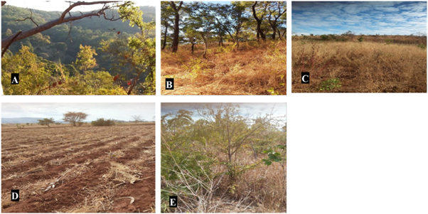
Figure 6. Typical land cover types for Thuma. Closed forest (A), Open forest (B), Savanna grassland (C), Shrubland (D) and Agriculture (E), Thuma forest reserve area, Malawi, Africa.
Download figure:
Standard image High-resolution image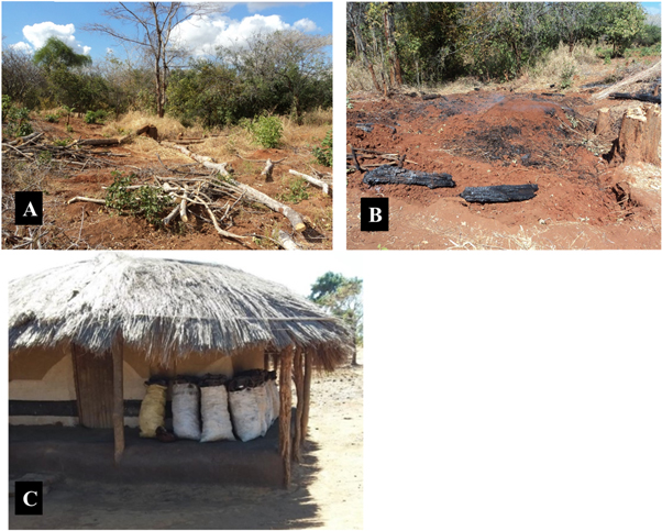
Figure 7. Newly opened agricultural field (A), charcoal processing 'furnace' (B) in open forest and charcoal ready (C) for sell or use in Kanyama Village close to Thuma Forest Reserve, Malawi, Africa.
Download figure:
Standard image High-resolution image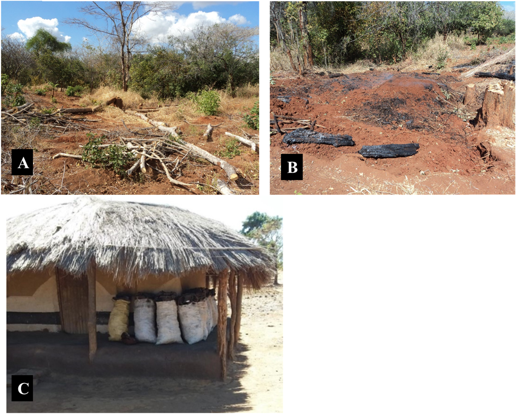
The loss in shrubland could be attributed to the fact that tobacco-growing farmers around the catchment cut down the small sized trees for use in tobacco curing and drying (Manyanhaire and Kurangwa 2014). This can also be attributed to use of shrubs for burning of bricks for house construction. As the shrubland decreases, savanna grassland is increasing. This could indicate a shift in cover change due to intense removal of the shrubs. A transition of land cover change from forest to bushes and shrubland has been reported in West Africa (Kusimi 2015). Although 30.9% of agriculture land went to savanna grassland from 1997–2007, almost the same area (30.5%) was converted to agriculture from 2007–2017. This could be attributed to the population increase in the four districts surrounding Thuma area (National Statistics Office 2018). From 1997–2017, the population in Dedza almost doubled from 486,682 to 830,512. In Salima, the population doubled from 248,214 to 478,346. Lilongwe and Dowa registered increases from 440,471 to 989,318 and 411,387 to 772,569 respectively. In most African countries, increased population has led to increased farm land expansion which leads to encroachment into some protected forest area (Smith et al 2016). It is also observed that there is more opening of agriculture fields in the areas with more people i.e. major village areas. The actual changes in land cover are as a result of direct causes (opening new crop land, settlement expansion, activities associated with mining, opening of new roads) and indirect factors (government policies, population growth) (Geist and Lambin 2002). Our findings are in tandem with those of Janssen et al (2018) and Appiah et al (2021) who reported high conversions from forest land to agriculture land in Tano-Offin and Kogya Forest Reserves respectively in Ghana. In southern Tanzania, Kayombo et al (2020), reported a land cover change from forest to shrubland, grassland and woodland for Image Forest Reserve area especially from 2004 to 2018. In Dedza District which shares boundary with Thuma area, forest area decreased as 61% was converted to barren land from 1991 to 2015 while 2.8% of the agriculture land was turned to built-environment (Munthali et al 2019).
More than 97% of the Malawi population uses unsustainable and illegal sources of biomass for domestic cooking (figures 7(B) and (C)) and heating energy (Environmental Affairs Department 2017). This is a challenge that needs both short and long-term strategies. The dwindling forest areas in Thuma should provide policymakers and natural resource managers the need to formulate both social and biophysical/ecological remedies to control the changes. It is apparent that the communities around Thuma area depend on the forest reserve for daily energy needs. It appears the 'land sparing' approach, where land is demarcated for specific use is slowly becoming unsuccessful and possibly there is a need to pursue 'land sharing', which entails the integration of more than two interventions (land uses) on a parcel of land (Loconto et al 2018). This could be achieved by encouraging farmers to engage in large-scale agroforestry where both targeted and naturally regenerating tree species should be managed at farm level. These trees should be the source of fuelwood energy by the communities. The approach of mixing crops and trees called Taungya in Ghana has been recorded to have reduced communities' reliance and level of encroachment in forest reserves (Acheampong et al 2016, Akamani and Hall 2019). This system stabilised the agricultural land cover such that from 2002 to 2017 the land lost from agriculture was equal to the land gained (Appiah et al 2021). Other options could revolve around subsidising of agricultural inputs to increase per unit production, strict bylaws, enforcement of national laws, and co-management. Such approaches will provide time for the recovery of the deforested forest reserves. Skole et al (2021), estimated that forest deforestation in Malawi ranges from 22,410 to 38,937 ha y−1.
Water class in this case represents surface water flowing in all the rivers and Linthipe and Linduzi rivers in the micro-catchments. Although, it was difficult to map the rivers accurately because their width was very small in the 30 m × 30 m pixel of Landsat image, the trend showed that the surface area of the rivers changed from 309.87 ha to 139.95 ha. This may have an effect on access to water by wildlife in Thuma area which may lead to migration of these game out of the area in search of water. Tree species that are endemic to water sources may also be reduced due to water loss. However, the change in the surface area of the rivers in the present study might be over or underestimated since some river portions are covered by trees, making it impossible for the satellite sensors to capture their exact spectral signature. Nonetheless, the change may be attributed to reduced cover that may have exacerbated soil erosion (that may have silted the rivers) or increased evaporation (Vargas and Omuto 2016).
5. Conclusion
Land cover and land use change assessment is crucial for sound decision-making at national and local level. The prominent land cover classes for Thuma forest reserve area (closed forest, open forest, shrubland, savanna grassland, agriculture and water) have shown changes from 1997, 2007 and 2017. The area under closed forest reduced from 7,000 ha to 3,000 ha while open forest shifted from 12,900 ha to 7,800 ha from 1997 to 2017 respectively. The area under savanna grassland has almost doubled from 5,900 ha to 13,000 ha. The area under agriculture has increased from 10,000 ha to 13,900 ha. By decadal percentage changes, closed forest changed from 19% in 1997 to 11% in 2007 to 6% in 2017, as agriculture area wobbled from 24% in 1997 to 21% in 2007 and 33% in 2017. The savanna area doubled from 13% in 1997 to 31% in 2017. The change from forest, shrubland, grassland to agriculture clearly shows ecosystem transition which has an impact on the biodiversity of both plants and animals. Future studies should integrate the changes with the associated drivers. The studies should also incorporate different data sets for ease of comparison. We recommend the use of Sentinel images which have a higher resolution of up to 10 m than Landsat 5 and 8. Sentinel images could help fully understand changes, especially water bodies which were not thorough in the present study. This study serves as a harbinger to government and relevant institutions for the need to put in place strategies that will buttress the successful management of Thuma forest reserve area. With the unique tree species diversity in the reserve and the fact that the reserve is currently used as a refuge for elephants, there is a need to ensure appropriate and timely remedies for the recession of the conversion of the reserve area into other land uses like farming. The reserve plays important role in maintaining the ecological status of important rivers, Linthipe and Linduzi. Linthipe River is a breeding niche for the endangered Opsaridium microlepis (locally called Mpasa) and Opsaridium microcephalis (locally called Sanjika) fish species. Based on this study, issues of re-demarcation of the area may also be explored. Programmes on forest landscape restoration through afforestation or regeneration should be considered to halt deforestation.
Acknowledgments
We appreciate the administrative roles by the management of United Nations Land Restoration Training Programme (UNU-LRT) during the execution of this study. We particularly thank Mr D Chonongera for assisting in field data collection. Many thanks to all the community members we interacted with during the field validation exercise.
Data availability statement
The data that support the findings of this study are available upon reasonable request from the authors.
Appendix A.: Field validation points
| Point | Latitude | Longitude | Point | Latitude | Longitude |
|---|---|---|---|---|---|
| 0 | 8479544 | 637080 | 30 | 8464022 | 622703 |
| 1 | 8478643 | 636826 | 31 | 8466521 | 622782 |
| 2 | 8478621 | 630827 | 32 | 8470487 | 626905 |
| 3 | 8477006 | 629765 | 33 | 8470868 | 627355 |
| 4 | 8478851 | 636110 | 34 | 8471122 | 627699 |
| 5 | 8478261 | 631961 | 35 | 8475154 | 640439 |
| 6 | 8476936 | 635164 | 36 | 8476030 | 640462 |
| 7 | 8474283 | 631819 | 37 | 8474258 | 641220 |
| 8 | 8472852 | 631519 | 38 | 8474385 | 641859 |
| 9 | 8479174 | 634957 | 39 | 8477481 | 635515 |
| 10 | 8474648 | 640823 | 40 | 8477821 | 634864 |
| 11 | 8468006 | 624760 | 41 | 8476662 | 634826 |
| 12 | 8464608 | 622728 | 42 | 8478005 | 634556 |
| 13 | 8453449 | 640846 | 43 | 8476417 | 634703 |
| 14 | 8454046 | 641284 | 44 | 8477135 | 632879 |
| 15 | 8454484 | 641837 | 45 | 8476493 | 633723 |
| 16 | 8456777 | 643139 | 46 | 8476856 | 633294 |
| 17 | 8457685 | 643412 | 47 | 8477733 | 632366 |
| 18 | 8454891 | 637792 | 48 | 8461270 | 623119 |
| 19 | 8457056 | 638681 | 49 | 8461604 | 622954 |
| 20 | 8456605 | 635499 | 50 | 8463649 | 622942 |
| 21 | 8458529 | 635950 | 51 | 8462595 | 623056 |
| 22 | 8460174 | 636310 | 52 | 8465635 | 622282 |
| 23 | 8463306 | 638876 | 53 | 8461525 | 637240 |
| 24 | 8464177 | 638843 | 54 | 8462185 | 638271 |
| 25 | 8470162 | 640746 | 55 | 8476794 | 629972 |
| 26 | 8469425 | 641170 | 56 | 8476135 | 629666 |
| 27 | 8467582 | 640162 | 57 | 8476028 | 629611 |
| 28 | 8455170 | 635501 | 58 | 8475021 | 630992 |
| 29 | 8453423 | 635730 | 59 | 8475342 | 632262 |
Appendix B.: Landsat Spectral bands and their properties. Source: from Horning 2004
| Band | Range | Characteristics |
|---|---|---|
| 1 | 0.45–0.52 μm, blue-green | Provides increased penetration of water bodies and is capable of differentiating soil and rock surfaces from vegetation and detecting cultural features |
| 2 | 0.52–0.60 μm, green | It matches the wavelength for the green we see when looking at vegetation. |
| It covers the green reflectance peak from leaf surfaces it separates vegetation from soil. | ||
| 3 | (0.63–0.69 μm, red | Vegetation absorbs nearly all red light (it is sometimes called the chlorophyll absorption band) this band can be useful for distinguishing between vegetation and soil and in monitoring vegetation health. |
| 4 | 0.76–0.90 μm, near infrared | Water absorbs nearly all light at this wavelength water bodies appear very dark. This contrasts with bright reflectance for soil and vegetation, so it is a good band for defining the water/land interface. Band |
| 5 | 1.55–1.75 μm, mid-infrared | This band is very sensitive to moisture and is therefore used to monitor vegetation and soil moisture. It is also good at differentiating between clouds and snow. Band |
| 6 | 10.40–12.50 μm, thermal infrared | This is a thermal band, it is used to measure surface temperature. This is primarily used for geological applications, but it is sometime used to measure plant heat stress. This is also used to differentiate clouds from bright soils since clouds tend to be very cold. One |
| 7 | 2.08–2.35 μm mid-infrared | This band is used for vegetation moisture as well as for soil and geology mapping. |