
Abstract
The Zernike polynomials are a complete set of continuous functions orthogonal over a unit circle. Since first developed by Zernike in 1934, they have been in widespread use in many fields ranging from optics, vision sciences, to image processing. However, due to the lack of a unified definition, many confusing indices have been used in the past decades and mathematical properties are scattered in the literature. This review provides a comprehensive account of Zernike circle polynomials and their noncircular derivatives, including history, definitions, mathematical properties, roles in wavefront fitting, relationships with optical aberrations, and connections with other polynomials. We also survey state-of-the-art applications of Zernike polynomials in a range of fields, including the diffraction theory of aberrations, optical design, optical testing, ophthalmic optics, adaptive optics, and image analysis. Owing to their elegant and rigorous mathematical properties, the range of scientific and industrial applications of Zernike polynomials is likely to expand. This review is expected to clear up the confusion of different indices, provide a self-contained reference guide for beginners as well as specialists, and facilitate further developments and applications of the Zernike polynomials.
Export citation and abstract BibTeX RIS

Original content from this work may be used under the terms of the Creative Commons Attribution 4.0 license. Any further distribution of this work must maintain attribution to the author(s) and the title of the work, journal citation and DOI.
1. Introduction
The Zernike polynomials are a sequence of continuous functions that form a complete orthogonal set over a unit disk. They were named after the optical physicist Frits Zernike (figure 1), winner of the 1953 Nobel Prize in Physics and the inventor of phase-contrast microscopy. Since most optical systems have circular apertures, Zernike polynomials are useful for wavefront analysis and thus play important roles in optics. Zernike polynomials can be generally divided into two basic types, i.e. Zernike circle polynomials and Zernike annular polynomials, which are defined over a unit disk and an annular unit disk, respectively. The Zernike circle polynomials were first introduced by Zernike in 1934 as eigenfunctions of a second-order rotationally invariant partial differential equation to describe the phase contrast method [1, 2] and were derived by Bhatia and Wolf in 1954 from the requirements of orthogonality and invariance [3]. The Zernike annular polynomials first appeared in a report of Perkin-Elmer Corporation in 1971 [4] and were discussed by Tatian in 1976 for aberrations balancing in optical systems with annular pupils from the standpoint of lens design [5]. They are systematically studied and explicitly given by Mahajan in 1981 [4].

Figure 1. Frits Zernike (1888–1966), a Dutch physicist and mathematician who was awarded the Nobel Prize in Physics in 1953 for his invention of the phase contrast microscope. Figure reproduced with permission from [7]. Reprinted from [7], Copyright © 2012 Elsevier B.V. All rights reserved.
Download figure:
Standard image High-resolution imageZernike polynomials gradually aroused people's interests after introduction (figure 2) and have found widespread applications in optics and image processing. In 1942, Bernard Nijboer, a PhD student of Zernike, expanded aberration functions of a symmetrical optical system into a series of Zernike polynomials and formulated an efficient representation of the complex amplitude distribution of a point object in the image plane [6]. This work allows analytical evaluation of diffraction integrals and the point spread function (PSF) of a general optical system and is referred to as the Nijboer–Zernike theory. However, the Nijboer–Zernike theory is only valid in the case of small aberrations and can only produce accurate results at positions close to geometrical focus. Seventy years later, Janssen formulated a general expression in terms of power-Bessel series and extended the Nijboer–Zernike theory for optical systems with large aberrations [8]. The extended Nijboer–Zernike theory can analytically compute the PSF of an aberrated optical system described by Zernike coefficients and accelerates further developments in the focused field diffraction theory. While the developments of diffraction theory of aberrations solely rely on analytical derivations, Zernike polynomial-based wavefront analysis depends on the use of computers. In the 1970s, with the rise of adaptive optics, Noll proposed a modified set of Zernike polynomials by normalizing and sorting the polynomials for statistical analysis of wavefront aberrations caused by atmospheric turbulence [9]. At the same time, Loomis at the University of Arizona introduced a reordered subset of Zernike polynomials to the interferogram processing software FRINGE for wavefront analysis in interferometric measurements [10, 11]. This subset called Zernike fringe set contains only 37 terms but has good corresponding relationships with classical aberrations. In 1980, Teague extended the applications of Zernike polynomials from optics to image processing and pioneered Zernike moments, which hold the property of rotation invariance and can be used as shape descriptors for pattern recognition [12]. The Zernike moments have since then become a valuable shape descriptor for image analysis. After entering the 21st century, the developments of Zernike polynomials gradually become mature and several Zernike sets were standardized to promote effective communication by the American National Standards Institute (ANSI) [13, 14] and the International Organization for Standardization (ISO) [15–17] (see figure 3).
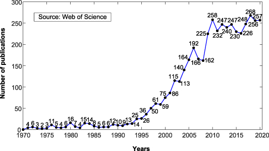
Figure 2. Number of publications on Zernike polynomials from 1970 to 2020. Source: Web of Science; keyword: Zernike polynomials; search criteria: topic.
Download figure:
Standard image High-resolution image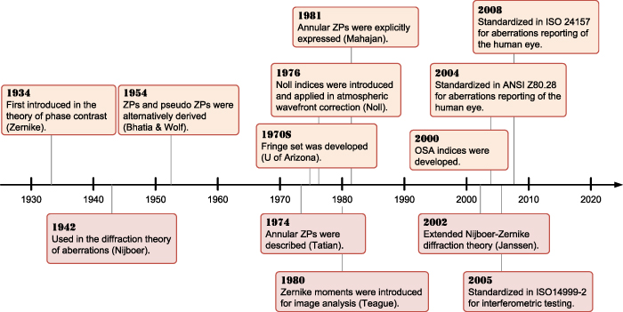
Figure 3. Key events in the history of Zernike polynomials (ZPs).
Download figure:
Standard image High-resolution imageThe widespread use of Zernike polynomials stems from their unique mathematical properties. First, Zernike polynomials are orthogonal over a unit circle. The orthogonality makes the expansion coefficients of a wavefront function independent of the number of terms [18]. This also enables convenient mathematical manipulations of wavefronts, such as addition, subtraction, translation, rotation, and scaling. Second, while other polynomials orthogonal over a unit disk also exist, Zernike polynomials are unique in the sense that they have good corresponding relationships with classical aberrations, such as astigmatism, coma, and spherical aberration [19, 20]. This enables fast classifications and quantifications of wavefront aberrations. Third, Zernike polynomials make the evaluation of the image quality of an optical system easy since the system PSF can be analytically computed from the Zernike expansion coefficients of wavefront aberrations based on the (extended) Nijboer–Zernike theory [6, 8, 21]. In addition, Zernike polynomials can serve as a basis set for wavefront reconstruction in slope sensitive wavefront sensors, such as the Shack–Hartmann wavefront slope sensor [22, 23] and the lateral shearing interferometers [24], which are important wavefront sensing tools in ophthalmic optics and adaptive optics.
Nowadays, a variety of indices for Zernike polynomials are in use by authors and authorities around the world. Well-known ones include the Noll indices [9, 25], the OSA/ANSI indices [13–15, 17, 26, 27], the Fringe/University of Arizona indices [10, 19], the ISO 14999 indices [16, 28], the Born and Wolf indices [29], and the Malacara indices [30, 31]. Each indexing scheme adopts a different naming, normalization, and indexing strategy and even the coordinate system may be different, which causes great confusion to researchers working with the polynomials and hinders effective communication. Moreover, mathematical properties of Zernike polynomials developed in the past few decades, such as derivatives, Fourier transform, and recurrence relations, are scattered in the literature and no work summarizes these results. This motivates us to prepare a review paper on the Zernike polynomials with the aims of clearing up the confusion of different indices, summarizing mathematical properties, surveying state-of-the-art applications, and providing a quick reference guide for scientists and engineers in this community.
The remainder of this review is organized as follows (see figure 4). Section 2 reviews different indexing schemes for the Zernike circle polynomials, their mathematical properties, roles in wavefront fitting, relationships with classical Seidel aberrations and the Strehl ratio, connections with other important functions, such as the XY monomials and the Legendre polynomials. Section 3 discusses orthonormal polynomials over noncircular pupils based on the Zernike circle polynomials with an emphasis on Zernike annular polynomials, whose definition, mathematical properties, and roles in wavefront fitting are presented. Section 4 surveys state-of-the-art applications of Zernike polynomials in a range of fields, including diffraction theory, optical design, optical testing, ophthalmic optics, adaptive optics, and image analysis. Finally, section 5 draws concluding remarks. Table 1 lists the acronyms and symbols used in this review.

Figure 4. Major topics discussed in this review.
Download figure:
Standard image High-resolution imageTable 1. List of acronyms and symbols.
| Symbols | Meaning |
|---|---|
| 3D | Three-dimensional |
| PSF | Point spread function |

| Cartesian coordinates and polar version in the spatial domain |

| Cartesian coordinates and polar version in the frequency domain |

| Orthonormal polynomials over arbitrary pupil shapes |

| Zernike resizing factor |
| I | Intensity; moment invariants |

| Bessel functions |

| Zernike moments |

| Normalization factor |

| Jacobi polynomials |

| Legendre polynomials |

| Pupil function |

| Zernike radial polynomials |

| XY monomials |

| Complex amplitude on the image plane |
| Un | Chebyshev polynomials |

| Complex Zernike circle polynomials of degree n with an azimuthal frequency l |

| Wavefront aberration |

| Wavefront mean value |
| Zernike circle polynomials of degree n with an azimuthal frequency m |
| Zernike annular polynomials with an obscuration ratio of 
|

| Phase function |

| Zernike expansion coefficients |

| Transformed Zernike expansion coefficients |

| Original images |

| Degraded images |

| Weighting factor for (complex) annular Zernike radial polynomials |

| Basis functions |

| Pseudo Zernike moments |

| Pseudo Zernike radial polynomials |

| Radon transform of Zernike radial polynomials |

| Pseudo Zernike polynomials |

| Fourier transform of Zernike circle polynomials |

| Fourier transform of Zernike annular polynomials |

| Coefficient matrix |

| Zernike expansion coefficients vector |

| Wavefront vector |

| Wavefront slope vector |
2. Zernike polynomials over circular pupils
2.1. Definitions
Zernike polynomials over circular pupils are called Zernike circle polynomials or simply Zernike polynomials. They are defined over a unit disk and can be most conveniently expressed in polar coordinates (ρ, θ), where ρ is the normalized radial coordinate (0 ⩽ ρ⩽ 1) and θ is the polar angle measured counterclockwise from the +x-axis (0 ⩽ θ < 2π), as shown in figure 5(a). The polar coordinates ρ and θ can be converted to the Cartesian coordinates x and y using the trigonometric functions:

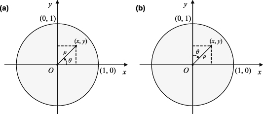
Figure 5. Definition of a unit circle: (a) Coordinate system used in this review. (b) Coordinate system not recommended.
Download figure:
Standard image High-resolution imageLikewise, the Cartesian coordinates x and y can be converted to polar coordinates ρ and θ by:
It is worth noting that while most people follow the convention that θ is positive when measured counterclockwise from the +x-axis, some authors, such as Born [32] and Malacara [30, 31], measure the polar angle from the +y-axis in the clockwise direction [33], which stems from early (pre-computer) aberration theory and is not recommended [27].
Zernike polynomials have several different indexing schemes during evolution, causing confusion to researchers, especially beginners. In this section, we classify indices in the literature into six groups, i.e. the Noll indices, the OSA/ANSI indices, the Fringe indices, the ISO 14999 indices, the Born and Wolf indices, and the Malacara indices, and compare their naming, normalization, and indexing strategies.
2.1.1. The Noll indexing scheme.
When Zernike first introduced the orthogonal polynomials, radial polynomials and azimuthal functions were explicitly given [1, 2]. However, the normalization and ordering methods for these polynomials were not specified. Noll in 1976 sorted and normalized Zernike polynomials to facilitate statistical analysis of wavefront distortion caused by atmospheric turbulence [9]. The indexing scheme was later followed by many authors [34–36] and was used in commercial software, such as Zemax [25] as the standard indices. Note that the 'standard' indices in Zemax are not associated with any ANSI or ISO standards. In this section, we summarize the Noll indexing scheme, discuss normalized and non-normalized Zernike circle polynomials, and extend the definitions from the real domain to the complex domain.
2.1.1.1. Real Zernike circle polynomials.
In the Noll indices, the normalized or orthonormal Zernike circle polynomials are defined as the products of normalization factors, radial polynomials, and azimuthal (angular) functions, which are written as [9]:
where the index n is the degree of the radial polynomials,  ; the index m is the azimuthal frequency describing the repetition of the angular function; n and m are non-negative integers and satisfy n − m⩾ 0 and n − m= even; j is a mode-ordering number starting from 1 and its relationships with n and m are presented in equation (8). There are a total of (n + 1)(n + 2)/2 linearly independent polynomials for a degree ⩽ n. The radial polynomial
  is defined as [1, 6]:
The radial polynomials of the first few degrees are shown in figure 6. It is easy to verify the following relations:

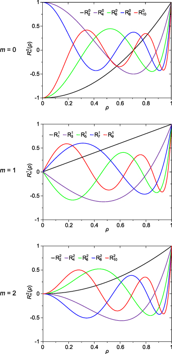
Figure 6. Zernike radial polynomials of the first few degrees when m = 0, 1, and 2.
Download figure:
Standard image High-resolution imageThe normalized Zernike circle polynomials meet the following orthonormality condition:
where  is the Kronecker delta function.
The orthonormal Zernike circle polynomials can be sorted by either the single index, j, or the double indices, n and m. The former is useful for describing Zernike expansion coefficients while the latter is useful for unambiguously describing the functions. To convert a given value j to n and m, one can use the following relationships [36]:
where ⌊x⌋ denotes the floor function that gives as output the greatest integer less than or equal to x. For example, ⌊2.4⌋ = 2. To convert given values of n and m to j, the following relationship can be used:
Table 2 lists the first 37-term real orthonormal Zernike circle polynomials in the polar and Cartesian coordinate systems and the values for n, m, and j.
Table 2. First 37-term orthonormal Zernike circle polynomials under the Noll indices [25, 36].
| j | n | m | Zj (ρ, θ) | Zj (x, y) | Aberration |
|---|---|---|---|---|---|
| 1 | 0 | 0 | 1 | 1 | Piston |
| 2 | 1 | 1 |

|

| x-tilt |
| 3 | 1 |

|

| y-tilt | |
| 4 | 2 | 0 |

|
![$\sqrt 3 [2({x^2} + {y^2}) - 1]$](https://content.cld.iop.org/journals/2040-8986/24/12/123001/revision3/joptac9e08ieqn44.gif)
| Defocus |
| 5 | 2 |

|

| 45° Primary astigmatism | |
| 6 | 2 |

|

| 0° Primary astigmatism | |
| 7 | 3 | 1 |

|
![$\sqrt 8 y[3({x^2} + {y^2}) - 2]$](https://content.cld.iop.org/journals/2040-8986/24/12/123001/revision3/joptac9e08ieqn50.gif)
| Primary y-coma |
| 8 | 1 |
|
![$\sqrt 8 x[3({x^2} + {y^2}) - 2]$](https://content.cld.iop.org/journals/2040-8986/24/12/123001/revision3/joptac9e08ieqn52.gif)
| Primary x-coma | |
| 9 | 3 |

|

| ||
| 10 | 3 |

|

| ||
| 11 | 4 | 0 |
|
![$\sqrt 5 [6{({x^2} + {y^2})^2} - 6({x^2} + {y^2}) + 1]$](https://content.cld.iop.org/journals/2040-8986/24/12/123001/revision3/joptac9e08ieqn58.gif)
| Primary spherical aberration |
| 12 | 2 |
|
![$\sqrt {10} ({x^2} - {y^2})[4({x^2} + {y^2}) - 3]$](https://content.cld.iop.org/journals/2040-8986/24/12/123001/revision3/joptac9e08ieqn60.gif)
| 0° Secondary astigmatism | |
| 13 | 2 |

|
![$2\sqrt {10} xy[4({x^2} + {y^2}) - 3]$](https://content.cld.iop.org/journals/2040-8986/24/12/123001/revision3/joptac9e08ieqn62.gif)
| 45° Secondary astigmatism | |
| 14 | 4 |

|
![$\sqrt {10} [{({x^2} + {y^2})^2} - 8{x^2}{y^2}]$](https://content.cld.iop.org/journals/2040-8986/24/12/123001/revision3/joptac9e08ieqn64.gif)
| ||
| 15 | 4 |

|
| ||
| 16 | 5 | 1 |
|
![$\sqrt {12} x[10{({x^2} + {y^2})^2} - 12({x^2} + {y^2}) + 3]$](https://content.cld.iop.org/journals/2040-8986/24/12/123001/revision3/joptac9e08ieqn68.gif)
| Secondary x-coma |
| 17 | 1 |

|
![$\sqrt {12} y[10{({x^2} + {y^2})^2} - 12({x^2} + {y^2}) + 3]$](https://content.cld.iop.org/journals/2040-8986/24/12/123001/revision3/joptac9e08ieqn70.gif)
| Secondary y-coma | |
| 18 | 3 |
|
![$\sqrt {12} x({x^2} - 3{y^2})[5({x^2} + {y^2}) - 4]$](https://content.cld.iop.org/journals/2040-8986/24/12/123001/revision3/joptac9e08ieqn72.gif)
| ||
| 19 | 3 |

|
![$\sqrt {12} y(3{x^2} - {y^2})[5({x^2} + {y^2}) - 4]$](https://content.cld.iop.org/journals/2040-8986/24/12/123001/revision3/joptac9e08ieqn74.gif)
| ||
| 20 | 5 |

|
![$\sqrt {12} x[16{x^4} - 20{x^2}({x^2} + {y^2}) + 5{({x^2} + {y^2})^2}]$](https://content.cld.iop.org/journals/2040-8986/24/12/123001/revision3/joptac9e08ieqn76.gif)
| ||
| 21 | 5 |

|
![$\sqrt {12} y[16{y^4} - 20{y^2}({x^2} + {y^2}) + 5{({x^2} + {y^2})^2}]$](https://content.cld.iop.org/journals/2040-8986/24/12/123001/revision3/joptac9e08ieqn78.gif)
| ||
| 22 | 6 | 0 |
|
![$\sqrt 7 [20{({x^2} + {y^2})^3} - 30{({x^2} + {y^2})^2} + 12({x^2} + {y^2}) - 1]$](https://content.cld.iop.org/journals/2040-8986/24/12/123001/revision3/joptac9e08ieqn80.gif)
| Secondary spherical |
| 23 | 2 |

|
![$2\sqrt {14} xy[15{({x^2} + {y^2})^2} - 20({x^2} + {y^2}) + 6]$](https://content.cld.iop.org/journals/2040-8986/24/12/123001/revision3/joptac9e08ieqn82.gif)
| 45° Tertiary astigmatism | |
| 24 | 2 |

|
![$\sqrt {14} ({x^2} - {y^2})[15{({x^2} + {y^2})^2} - 20({x^2} + {y^2}) + 6]$](https://content.cld.iop.org/journals/2040-8986/24/12/123001/revision3/joptac9e08ieqn84.gif)
| 0° Tertiary astigmatism | |
| 25 | 4 |

|
![$4\sqrt {14} xy({x^2} - {y^2})[6({x^2} + {y^2}) - 5]$](https://content.cld.iop.org/journals/2040-8986/24/12/123001/revision3/joptac9e08ieqn86.gif)
| ||
| 26 | 4 |

|
![$\sqrt {14} [{({x^2} + {y^2})^2} - 8{x^2}{y^2}][6({x^2} + {y^2}) - 5]$](https://content.cld.iop.org/journals/2040-8986/24/12/123001/revision3/joptac9e08ieqn88.gif)
| ||
| 27 | 6 |

|
![$\sqrt {14} xy[32{x^4} - 32{x^2}({x^2} + {y^2}) + 6{({x^2} + {y^2})^2}]$](https://content.cld.iop.org/journals/2040-8986/24/12/123001/revision3/joptac9e08ieqn90.gif)
| ||
| 28 | 6 |

|
![$\begin{gathered} \sqrt {14} [32{x^6} - 48{x^4}({x^2} + {y^2})\, + \\ 18{x^2}{({x^2} + {y^2})^2} - {({x^2} + {y^2})^3}] \\ \end{gathered} $](https://content.cld.iop.org/journals/2040-8986/24/12/123001/revision3/joptac9e08ieqn92.gif)
| ||
| 29 | 7 | 1 |

|
![$4y[35{({x^2} + {y^2})^3} - 60{({x^2} + {y^2})^2} + 30({x^2} + {y^2}) - 4]$](https://content.cld.iop.org/journals/2040-8986/24/12/123001/revision3/joptac9e08ieqn94.gif)
| Tertiary y-coma |
| 30 | 1 |

|
![$4x[35{({x^2} + {y^2})^3} - 60{({x^2} + {y^2})^2} + 30({x^2} + {y^2}) - 4]$](https://content.cld.iop.org/journals/2040-8986/24/12/123001/revision3/joptac9e08ieqn96.gif)
| Tertiary x-coma | |
| 31 | 3 |

|
![$4y(3{x^2} - {y^2})[21{({x^2} + {y^2})^2} - 30({x^2} + {y^2}) + 10]$](https://content.cld.iop.org/journals/2040-8986/24/12/123001/revision3/joptac9e08ieqn98.gif)
| ||
| 32 | 3 |

|
![$4x({x^2} - 3{y^2})[21{({x^2} + {y^2})^2} - 30({x^2} + {y^2}) + 10]$](https://content.cld.iop.org/journals/2040-8986/24/12/123001/revision3/joptac9e08ieqn100.gif)
| ||
| 33 | 5 |

|
![$\begin{gathered} 4[4{x^2}y({x^2} - {y^2}) + y{({x^2} + {y^2})^2} - 8{x^2}{y^3}]\\ \times [7({x^2} + {y^2}) - 6]\qquad\quad\qquad\quad\quad\quad\;\; \\ \end{gathered} $](https://content.cld.iop.org/journals/2040-8986/24/12/123001/revision3/joptac9e08ieqn102.gif)
| ||
| 34 | 5 |

|
![$\begin{gathered} 4[x{({x^2} + {y^2})^2} - 8{x^3}{y^2} - 4x{y^2}({x^2} - {y^2})]\, \\ \times[7({x^2} + {y^2}) - 6]\qquad\quad\qquad\quad\quad\quad\;\; \\ \end{gathered} $](https://content.cld.iop.org/journals/2040-8986/24/12/123001/revision3/joptac9e08ieqn104.gif)
| ||
| 35 | 7 |

|
![$\begin{gathered} 8{x^2}y[3{({x^2} + {y^2})^2} - 16{x^2}{y^2}]\,\;\quad\quad\;\; \\ + 4y({x^2} - {y^2})[{({x^2} + {y^2})^2} - 16{x^2}{y^2}] \\ \end{gathered} $](https://content.cld.iop.org/journals/2040-8986/24/12/123001/revision3/joptac9e08ieqn106.gif)
| ||
| 36 | 7 |

|
![$\begin{gathered} 4x({x^2} - {y^2})[{({x^2} + {y^2})^2} - 16{x^2}{y^2}] \\ - 8x{y^2}[3{({x^2} + {y^2})^2} - 16{x^2}{y^2}]\;\;\quad \\ \end{gathered} $](https://content.cld.iop.org/journals/2040-8986/24/12/123001/revision3/joptac9e08ieqn108.gif)
| ||
| 37 | 8 | 0 |

|
![$\begin{gathered} 3[70{({x^2} + {y^2})^4} - 140{({x^2} + {y^2})^3}\,\quad \\ + 90{({x^2} + {y^2})^2} - 20({x^2} + {y^2}) + 1] \\ \end{gathered} $](https://content.cld.iop.org/journals/2040-8986/24/12/123001/revision3/joptac9e08ieqn110.gif)
| Tertiary spherical |
The non-normalized real Zernike circle polynomials can be obtained by dropping the normalization factors from the normalized Zernike circle polynomials as:
They satisfy the following relationship:

The orthogonality of non-normalized Zernike circle polynomials can be written as:
Note that the integral in the denominator is equal to π. Figures 7 and 8 show the three-dimensional (3D) visualization of the non-normalized Zernike circle polynomials up to the sixth degree and their corresponding interferometric fringe patterns as in optical testing [37].
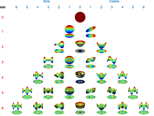
Figure 7. Pyramid of the non-normalized Zernike circle polynomials up to the sixth degree under the Noll indexing scheme.
Download figure:
Standard image High-resolution image
Figure 8. Interferometric fringe patterns corresponding to the Zernike aberrations shown in figure 7.
Download figure:
Standard image High-resolution image2.1.1.2. Complex Zernike circle polynomials.
The Zernike circle polynomials in the complex domain were not defined in Noll's original definition [9]. However, they can be obtained based on Bhatia and Wolf's work [3] by replacing the azimuthal functions in real Zernike circle polynomials with a complex exponential function. The orthonormal complex Zernike circle polynomials can be written as [4]:

where n is a non-negative integer, l is an integer, n − |l| ⩾ 0 and is even. The radial polynomial is defined as:
The normalized complex Zernike circle polynomials meet the following orthonormality condition:
where * denotes complex conjugate.
The non-normalized version of the complex Zernike circle polynomials are defined as [32]:

The orthogonality can be expressed as:
The complex and real definitions of Zernike circle polynomials are related via the Euler's formula [3, 32]. The complex version is useful to define Zernike moments in image analysis, which will be discussed in section 4.6.
2.1.2. The OSA/ANSI indexing scheme.
The OSA/ANSI indices for Zernike circle polynomials were initially developed by an OSA Standards Taskforce in 1999 to reach consensus recommendations on definitions, conventions, and standards for reporting of optical aberrations of human eyes [26, 27]. It was later standardized in ANSI Z80.28 [13, 14] and ISO 24157 [15, 17] and adopted in some commercial software, such as COMSOL Ray Optics Module [38].
The Zernike circle polynomials in the OSA/ANSI indices employ a right-handed coordinate system, as shown in figure 9, and are defined in the real domain as [13, 14, 26, 27].

Figure 9. Conventional right-handed coordinate system for the eye in Cartesian and polar forms.
Download figure:
Standard image High-resolution imagewhere n is a non-negative integer, m is an integer, n − |m| ⩾ 0 and is even, j is a mode-ordering number starting from 0. The radial polynomial,  , is defined as:
The normalization factor,  , can be written as:
The Zernike circle polynomials under the OSA/ANSI indices can be sorted by either the single index, j, or the double indices, n and m. To achieve conversion among these indices, one can use the following relationships [26, 27]:
where ⌈x⌉ denotes the ceiling function that gives as output the least integer greater than or equal to x. For example, when j = 4, n = ⌈1.7⌉ = 2, m = 0. Table 3 lists the first 37-term Zernike circle polynomials in the OSA/ANSI indices and the values for n, m, and j.
Table 3. First 37-term Zernike polynomials under the OSA/ANSI indices [14, 27, 39].
| j | n | m | Zj | Aberration |
|---|---|---|---|---|
| 0 | 0 | 0 | 1 | Piston |
| 1 | 1 | −1 |

| y-tilt |
| 2 | 1 |

| x-tilt | |
| 3 | 2 | −2 |

| 45° Primary astigmatism |
| 4 | 0 |

| Defocus | |
| 5 | 2 |

| 0° Primary astigmatism | |
| 6 | 3 | −3 |

| |
| 7 | −1 |
| Primary y-coma | |
| 8 | 1 |

| Primary x-coma | |
| 9 | 3 |

| ||
| 10 | 4 | −4 |

| |
| 11 | −2 |
| 45° Secondary astigmatism | |
| 12 | 0 |

| Primary spherical aberration | |
| 13 | 2 |

| 0° Secondary astigmatism | |
| 14 | 4 |

| ||
| 15 | 5 | −5 |

| |
| 16 | −3 |
| ||
| 17 | −1 |
| Secondary y-coma | |
| 18 | 1 |

| Secondary x-coma | |
| 19 | 3 |

| ||
| 20 | 5 |

| ||
| 21 | 6 | −6 |

| |
| 22 | −4 |
| ||
| 23 | −2 |

| 45° Tertiary astigmatism | |
| 24 | 0 |

| Secondary spherical | |
| 25 | 2 |

| 0° Tertiary astigmatism | |
| 26 | 4 |
| ||
| 27 | 6 |

| ||
| 28 | 7 | −7 |

| |
| 29 | −5 |

| ||
| 30 | −3 |

| ||
| 31 | −1 |

| Tertiary y-coma | |
| 32 | 1 |

| Tertiary x-coma | |
| 33 | 3 |

| ||
| 34 | 5 |
| ||
| 35 | 7 |

| ||
| 36 | 8 | −8 |

|
2.1.3. The Fringe indexing scheme.
The Zernike circle polynomials under the fringe indexing scheme (also known as the USAF set) were first developed by John Loomis in an interferogram analysis program called FRINGE at the University of Arizona, Optical Sciences Center in the 1970s [10, 11, 40, 41]. They are a low-order Zernike set supplemented with radial polynomials of higher order and are preferred for lens design and optical metrology because they group terms according to optical wavefront aberration order [42, 43].
The Zernike circle polynomials under the fringe indices do not have normalization factors and can be written as:
where n is a non-negative integer, m is an integer, n − |m| ⩾ 0 and is even, j is a mode-ordering number starting from 0 (In CODE V and Zemax, j starts from 1 instead of 0). The radial polynomial is expressed as:

Note that the above formulas are modified from the Wyant and Creath formula [19] to facilitate comparisons with other indices. The final mathematical expression for each term, as listed in table 4, is the same as that in Wyant's notation.
Table 4. Fringe set of the Zernike circle polynomials [19, 25, 29].
| j | N | n | m | Zj (ρ, θ) | Aberration |
|---|---|---|---|---|---|
| 0 | 0 | 0 | 0 | 1 | Piston |
| 1 | 1 | 1 | +1 |

| Tilt X |
| 2 | 1 | −1 |

| Tilt Y | |
| 3 | 2 | 0 |

| Defocus | |
| 4 | 2 | 2 | +2 |

| Astigmatism X |
| 5 | 2 | −2 |

| Astigmatism Y | |
| 6 | 3 | +1 |

| Coma X | |
| 7 | 3 | −1 |

| Coma Y | |
| 8 | 4 | 0 |

| Primary spherical | |
| 9 | 3 | 3 | +3 |

| Trefoil X |
| 10 | 3 | −3 |

| Trefoil Y | |
| 11 | 4 | +2 |

| Secondary X astigmatism | |
| 12 | 4 | −2 |

| Secondary Y astigmatism | |
| 13 | 5 | +1 |
| Secondary X coma | |
| 14 | 5 | −1 |

| Secondary Y coma | |
| 15 | 6 | 0 |
| Secondary spherical | |
| 16 | 4 | 4 | +4 |

| Tetrafoil X |
| 17 | 4 | −4 |

| Tetrafoil X | |
| 18 | 5 | +3 |

| Secondary X trefoil | |
| 19 | 5 | −3 |

| Secondary Y trefoil | |
| 20 | 6 | +2 |

| Tertiary X astigmatism | |
| 21 | 6 | −2 |
| Tertiary Y astigmatism | |
| 22 | 7 | +1 |

| Tertiary X coma | |
| 23 | 7 | −1 |

| Tertiary Y coma | |
| 24 | 8 | 0 |

| Tertiary spherical | |
| 25 | 5 | 5 | +5 |

| Pentafoil X |
| 26 | 5 | −5 |

| Pentafoil Y | |
| 27 | 6 | +4 |

| Secondary X Tetrafoil | |
| 28 | 6 | −4 |

| Secondary Y Tetrafoil | |
| 29 | 7 | +3 |
| Tertiary X Trefoil | |
| 30 | 7 | −3 |
| Tertiary Y Trefoil | |
| 31 | 8 | +2 |

| Quaternary X astigmatism | |
| 32 | 8 | −2 |

| Quaternary Y astigmatism | |
| 33 | 9 | +1 |

| Quaternary X coma | |
| 34 | 9 | −1 |

| Quaternary Y coma | |
| 35 | 10 | 0 |

| Quaternary Spherical | |
| 36 | 6 | 12 | 0 |

|
Defining N = (n + |m|)/2, Zernike fringe polynomials can be sorted as follows. First arrange N in ascending order from 0 to 6; then sort n in ascending order for a given value of N; finally organize m in descending order for given values of N and n. Compared with other Zernike sets, the Zernike fringe set is unique in the sense that it only has 37 terms (N ⩽ 6). This small polynomial set is useful for interferogram analysis and automatic lens design and is widely adopted in commercial optical software, such as Zemax [25], CODE V [29], OSLO [44, 45], and MetroPro [46].
2.1.4. The ISO-14999 indexing scheme.
The ISO-14999 indices were first published by ISO in the ISO/TR 14999–2 technical report in 2005 [28] for the description of wavefront in interferometric measurement of optical elements and optical system and then updated in 2019 [16].
The Zernike circle polynomials under the ISO-14999 indexing scheme do not have normalization factors and can be written as [16, 28]:
where n is a non-negative integer, m is an integer, n − |m| ⩾ 0 and is even, j is a mode-ordering number starting from 0 (j = 0, 1, 2, ..., ∞). The radial polynomial is expressed as:
Defining N = n + |m|, the Zernike circle polynomials under the ISO-14999 indices are sorted as follows. First arrange N in ascending order from 0 to ∞; then sort n in ascending order for a given value of N; finally organize m in descending order for given values of N and n. One may find that the ISO-14999 indices share almost the same definition as the fringe indices except that the former contains infinite terms. Actually, the fringe set is a subset of the ISO-14999 set, which is called the Extended Fringe Zernike Polynomials in CODE V [29]. Table 5 lists the first 37 terms of the ISO-14999 set and the values for n, m, N, and j.
Table 5. First 37-term Zernike circle polynomials under the ISO-14999 indices [16, 28].
| j | N | n | m | Zj | Aberration |
|---|---|---|---|---|---|
| 0 | 0 | 0 | 0 | 1 | Piston |
| 1 | 2 | 1 | 1 |

| x-Tilt |
| 2 | 1 | −1 |

| y-Tilt | |
| 3 | 2 | 0 |

| Defocus | |
| 4 | 4 | 2 | 2 |

| 0° Primary astigmatism |
| 5 | 2 | −2 |

| 45° Primary astigmatism | |
| 6 | 3 | 1 |
| Primary x-coma | |
| 7 | 3 | −1 |

| Primary y-coma | |
| 8 | 4 | 0 |

| Primary spherical aberration | |
| 9 | 6 | 3 | 3 |

| |
| 10 | 3 | −3 |

| ||
| 11 | 4 | 2 |

| 0° Secondary astigmatism | |
| 12 | 4 | −2 |

| 45° Secondary astigmatism | |
| 13 | 5 | 1 |

| Secondary x-coma | |
| 14 | 5 | −1 |
| Secondary y-coma | |
| 15 | 6 | 0 |

| Secondary spherical | |
| 16 | 8 | 4 | 4 |

| |
| 17 | 4 | −4 |

| ||
| 18 | 5 | 3 |

| ||
| 19 | 5 | −3 |

| ||
| 20 | 6 | 2 |

| 0° Tertiary astigmatism | |
| 21 | 6 | −2 |

| 45° Tertiary astigmatism | |
| 22 | 7 | 1 |

| Tertiary x-coma | |
| 23 | 7 | −1 |

| Tertiary y-coma | |
| 24 | 8 | 0 |

| Tertiary spherical | |
| 25 | 10 | 5 | 5 |

| |
| 26 | 5 | −5 |

| ||
| 27 | 6 | 4 |
| ||
| 28 | 6 | −4 |
| ||
| 29 | 7 | 3 |

| ||
| 30 | 7 | −3 |

| ||
| 31 | 8 | 2 |

| 0° Quaternary astigmatism | |
| 32 | 8 | −2 |

| 45° Quaternary astigmatism | |
| 33 | 9 | 1 |

| Quaternary x-coma | |
| 34 | 9 | −1 |

| Quaternary y-coma | |
| 35 | 10 | 0 |

| Quaternary spherical | |
| 36 | 12 | 6 | 6 |

|
2.1.5. The Born and Wolf indexing scheme.
In the classic textbook Principle of Optics, Born and Wolf reviewed the definition of Zernike circle polynomials and used it for the expansion of aberration functions [32, 47]. Many people [12, 48] later follow the Born and Wolf definition and treat it as the 'standard' indexing scheme. However, as pointed out in Born and Wolf's book (appendix VII in the 7th expanded edition [32]), the indices actually originated from Bhatia and Wolf's work published in 1954 [3].
The Zernike circle polynomials under the Born and Wolf indices do not have normalization factors and can be written as [3, 32]:
where n is a non-negative integer, m is an integer, n − |m| ⩾ 0 and is even, j is a mode-ordering number starting from 1 (j = 1, 2, ..., ∞). The radial polynomial is expressed as:
The Zernike circle polynomials under the Born and Wolf indices are sorted as follows. First arrange n in ascending order from 0 to ∞ and then sort m in descending order for a given value of n. The Born and Wolf indices are used by several authors [12, 48] and software [29]. For example, although the software CODE V does not explicitly define the standard Zernike polynomials, the tabulated polynomials in its manual [29] have the same expressions as those in the Born and Wolf indices. Table 6 lists the first 37-term Zernike polynomials under the Born and Wolf indices and the values for n, m, and j.
Table 6. First 37-term Zernike circle polynomials under the Born and Wolf indices [29].
| j | n | m | Zj (ρ, θ) | Aberration |
|---|---|---|---|---|
| 1 | 0 | 0 | 1 | Piston |
| 2 | 1 | 1 |

| x-tilt |
| 3 | −1 |

| y-tilt | |
| 4 | 2 | 2 |

| 0° Primary astigmatism |
| 5 | 0 |

| Defocus | |
| 6 | −2 |

| 45° Primary astigmatism | |
| 7 | 3 | 3 |

| |
| 8 | 1 |

| Primary x-coma | |
| 9 | −1 |
| Primary y-coma | |
| 10 | −3 |

| ||
| 11 | 4 | 4 |

| |
| 12 | 2 |
| 0° Secondary astigmatism | |
| 13 | 0 |

| Primary spherical aberration | |
| 14 | −2 |

| 45° Secondary astigmatism | |
| 15 | −4 |

| ||
| 16 | 5 | 5 |

| |
| 17 | 3 |

| ||
| 18 | 1 |

| Secondary x-coma | |
| 19 | −1 |

| Secondary y-coma | |
| 20 | −3 |

| ||
| 21 | −5 |

| ||
| 22 | 6 | 6 |

| |
| 23 | 4 |

| ||
| 24 | 2 |

| 0° Tertiary astigmatism | |
| 25 | 0 |

| Secondary spherical | |
| 26 | −2 |

| 45° Tertiary astigmatism | |
| 27 | −4 |

| ||
| 28 | −6 |

| ||
| 29 | 7 | 7 |

| |
| 30 | 5 |

| ||
| 31 | 3 |

| ||
| 32 | 1 |

| Tertiary x-coma | |
| 33 | −1 |

| Tertiary y-coma | |
| 34 | −3 |

| ||
| 35 | −5 |
| ||
| 36 | −7 |

| ||
| 37 | 8 | 8 |

|
2.1.6. The Malacara indexing scheme.
Different from the aforementioned five indexing schemes, the Malacara indices use a different coordinate convention, where the polar angle, θ, is measured clockwise from the +y-axis. The Zernike circle polynomials under the Malacara indices do not have normalization factors and can be written as:
where n is a non-negative integer, m is an integer, n − |m| ⩾ 0 and is even, j is a mode-ordering number starting from 1 (j = 1, 2, ..., ∞). The radial polynomial is expressed as:
The Zernike circle polynomials in the Malacara indices have the same ordering scheme as the Born and Wolf indices and are sorted as follows. First arrange n in ascending order from 0 to ∞ and then sort m in descending order for a given value of n. The Malacara indices are mainly used in the first and second editions of the well-known book Optical Shop Testing [30, 31], the third edition of which, however, defines the Zernike circle polynomials under the Noll indexing scheme [36]. Table 7 lists the first 37-term Zernike circle polynomials under the Malacara indices and the values for n, m, and j.
Table 7. First 37-term Zernike circle polynomials under the Malacara indices [31].
| j | n | m | Zj (ρ, θ) | Aberration |
|---|---|---|---|---|
| 1 | 0 | 0 | 1 | Piston |
| 2 | 1 | 1 |

| x-tilt |
| 3 | −1 |

| y-tilt | |
| 4 | 2 | 2 |

| 0° Primary astigmatism |
| 5 | 0 |

| Defocus | |
| 6 | −2 |

| 45° Primary astigmatism | |
| 7 | 3 | 3 |

| |
| 8 | 1 |

| Primary x-coma | |
| 9 | −1 |

| Primary y-coma | |
| 10 | −3 |

| ||
| 11 | 4 | 4 |

| |
| 12 | 2 |
| 0° Secondary astigmatism | |
| 13 | 0 |

| Primary spherical aberration | |
| 14 | −2 |

| 45° Secondary astigmatism | |
| 15 | −4 |

| ||
| 16 | 5 | 5 |

| |
| 17 | 3 |
| ||
| 18 | 1 |

| Secondary x-coma | |
| 19 | −1 |

| Secondary y-coma | |
| 20 | −3 |
| ||
| 21 | −5 |

| ||
| 22 | 6 | 6 |

| |
| 23 | 4 |

| ||
| 24 | 2 |

| 0° Tertiary astigmatism | |
| 25 | 0 |

| Secondary spherical | |
| 26 | −2 |
| 45° Tertiary astigmatism | |
| 27 | −4 |

| ||
| 28 | −6 |

| ||
| 29 | 7 | 7 |

| |
| 30 | 5 |

| ||
| 31 | 3 |

| ||
| 32 | 1 |

| Tertiary x-coma | |
| 33 | −1 |

| Tertiary y-coma | |
| 34 | −3 |

| ||
| 35 | −5 |
| ||
| 36 | −7 |

| ||
| 37 | 8 | 8 |

|
2.1.7. Comparisons.
The different indexing schemes of Zernike circle polynomials are compared and summarized in table 8 from the perspectives of coordinate system, normalization, and ordering strategy. In particular, the sorting of the polynomials under different indices is shown in figure 10 for the first few degrees. An illustration of the sources and applications of the six indices is presented in figure 11. For convenience, the Noll indices will be used in the remaining part of the article unless otherwise stated.
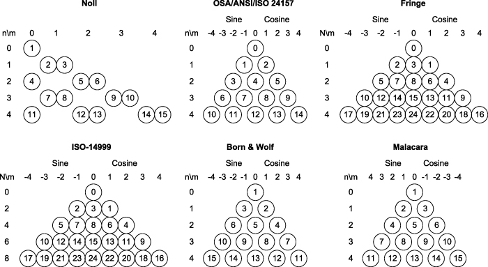
Figure 10. Comparison of the low-order sequences of different indices.
Download figure:
Standard image High-resolution image
Figure 11. Summary of the different indexing schemes and their sources. ZPs: Zernike polynomials.
Download figure:
Standard image High-resolution imageTable 8. Comparison of different indices for Zernike circle polynomials in the real domain.
| Noll | OSA/ANSI | Fringe/U of Arizona | ISO-14999 | Born and Wolf | Malacara | |
|---|---|---|---|---|---|---|
| Sources | Noll, 1976 [9] Zemax Standard ZPs [25] Optical Shop Testing (3rd ed), 2007 [36] | OSA VSIA Standards Taskforce, 2000 [26] ANSI Z80.28 [13, 14] ISO 24157 [15, 17] COMSOL Ray Optics Module [38] | Loomis, 1970s [10, 49]
Wyant, 1992 [19]
Zemax Fringe ZPs | ISO/TR 14999–2, 2005 [16, 28]
CODE V Extended Fringe ZPs | Bhatia and Wolf, 1954 [3] Born and Wolf, 1964 [50] CODE V Standard ZPs [29] | Optical Shop Testing (1st & 2nd eds), 1978 and 1992 [30, 31] |
| Domain | Real | Real | Real | Real | Real | Real |
| Coordinate system | 0 ⩽ ρ ⩽ 1, θ from +x axis anticlockwise | 0 ⩽ ρ ⩽ 1, θ from +x axis anticlockwise | 0 ⩽ ρ ⩽ 1, θ from +x axis anticlockwise | 0 ⩽ ρ ⩽ 1, θ from +x axis anticlockwise | 0 ⩽ ρ ⩽ 1, θ from +x axis anticlockwise | 0 ⩽ ρ ⩽ 1, θ from +y axis clockwise |
| Definition |
|
|

|

|
|
|
| Radial polynomial |
|
| ||||
| Normalization | Yes | Yes | No | No | No | No |
| Normalization factor |
|

| — | — | — | — |
| Term number | Infinite | Infinite | 37 | Infinite | Infinite | Infinite |
| Double indices | n: non-negative integer m: non-negative integer n − m ⩾ 0 and even | n: non-negative integer m: integer n − |m| ⩾ 0 and even | n: non-negative integer m: integer n − |m| ⩾ 0 and even N = (n + |m|)/2 | n: non-negative integer m: integer n−|m| ⩾ 0 and even N = n + |m| | n: non-negative integer m: integer n−|m| ⩾ 0 and even | n: non-negative integer m: integer n−|m| ⩾ 0 and even |
| Single index | j = 1, 2, 3, ..., ∞ | j = 0, 1, 2, ..., ∞ | j = 0, 1, 2, ..., 36 | j = 0, 1, 2, ..., ∞ | j = 1, 2, 3, ..., ∞ | j = 1, 2, 3, ..., ∞ |
| Indexing scheme | n from 0 to ∞ m in ascending order | n from 0 to ∞ m in ascending order | N from 0 to 6 n in ascending order m in descending order | N from 0 to ∞ n in ascending order m in descending order | n from 0 to ∞ m in descending order | n from 0 to ∞ m in descending order |
| Major applications | General optics | Ophthalmic optics | Optical metrology | Optical metrology | Optical design | Rarely used |
a In CODE V and Zemax, the single index j for the fringe Zernike polynomials (ZPs) starts from 1. b In OSLO, the polar angle θ is measured from the +y axis [44].
2.2. Mathematical properties
In this section, we review major mathematical properties of Zernike circle polynomials, including orthogonality, symmetry, Fourier transform, integral representation of radial polynomials, derivatives, and recurrence relations. For more properties, one can refer to [51, 52].
2.2.1. Orthogonality.
The orthogonal relationships of real and complex Zernike circle polynomials have been presented and can be found in equations (7), (12), (15) and (17). Moreover, the radial and azimuthal functions of Zernike circle polynomials are also orthogonal and satisfy the following relationships [36]:
Note that the Noll indices are used here.
2.2.2. Symmetry.
The symmetry of Zernike circle polynomials can be expressed as:

2.2.3. The Fourier transform.
Define the Fourier transform pair as:


where  is the Fourier transform of Zj
and (u, v) are Cartesian coordinates in the frequency domain. Use (r, φ) to denote the polar coordinates in the frequency domain and apply the transformation relationships x = ρcosθ, y = ρsinθ, u = rcosφ, v = rsinφ, the Fourier transform of Zernike circle polynomials can be written as [9, 53]:
is the Fourier transform of Zj
and (u, v) are Cartesian coordinates in the frequency domain. Use (r, φ) to denote the polar coordinates in the frequency domain and apply the transformation relationships x = ρcosθ, y = ρsinθ, u = rcosφ, v = rsinφ, the Fourier transform of Zernike circle polynomials can be written as [9, 53]:
where Jn (x) is the nth-order Bessel function of the first kind and is defined as [54]:
The Fourier transform of Zernike circle polynomials is useful for the conversion between Zernike coefficients and Fourier series coefficients of a wavefront [53].
2.2.4. Integral representation of radial polynomials.
Substituting equation (35) into the inverse Fourier transform of Zernike circle polynomials (equation (34)), an integral representation of Zernike radial polynomials can be obtained as [2, 6]:
This integral representation is useful for deriving a recurrence relation of the derivatives of Zernike radial polynomials [9].
2.2.5. Derivatives.
The integral representation for the radial polynomials provides a good starting point for calculating derivatives. The derivatives of radial polynomials can be written in a recursion relation as [9]:
In polar coordinate system, the partial derivatives of Zernike circle polynomials under the Noll indices with respect to x and y can be written as [18, 55]:
where the normalization factor and the azimuthal function are:
In Cartesian coordinate system, the partial derivatives of Zernike circle polynomials under the OSA/ANSI indices with respect to x and y can be written as [14]:
where n' increases with a step of 2 in the summations and in the case that (|m| + 1) is larger than (n − 1), the first summation term does not exist. The Cartesian derivatives of Zernike circle polynomials can also be obtained using recurrence relations, as reported in [55–57]. The derivatives of Zernike circle polynomials are useful for certain problems, such as ray tracing in optical design [58] and wavefront reconstruction in wavefront sensing [22, 24].
2.2.6. Recurrence relations.
Computation of high-order of Zernike circle polynomials is necessary for some applications, such as Zernike moments-based image analysis. Although the radial polynomials are explicitly formulated (equation (19)), direct numerical computation suffers from the problem of low computational efficiency and possible cancellation errors [59–61]. To deal with these problems, various recurrence relations have been proposed for evaluating the radial polynomials [60–64]. Here we briefly review four widely-used recurrence methods, including the modified Kintner method [59, 65], the Prata's method [66], the q-recursive method [59], and the Shakibaei and Paramesran method [62].
The modified Kintner method was first proposed by Kintner in 1976 [65] and improved by Chong et al in 2003 [59] by adding recurrence relations for special cases when n − m = 0 and 2. The improved recurrence relation can be expressed as:
where n and m are non-negative integers and satisfy n − m ⩾ 0 and n − m = even; the coefficients are given by:
The modified Kintner method is a degree-varying (n-varying) approach that computes radial polynomials at higher order from those at lower order for a fixed value of m.
The Prata method was proposed by Prata and Rusch in 1989 [66] and the recurrence relation can be written as:
where,
The q-recursive method was proposed by Chong et al [59] and the three-term recurrence relation can be written as:
where the coefficients are given by:
Different from the modified Kintner method and the Prata method, the q-recursive method is an m-varying method that computes radial polynomials at lower m from those at higher m for a fixed radial order n.
The Shakibaei and Paramesran method uses a particularly simple recursion, in which a radial polynomial is expressed as a linear combination of three earlier computed radial polynomials as [62]:

The recursion can be initialized with the conditions  and
and  when n < m. According to [67], the speed and accuracy of the recursion outperforms the Prata method and the q-recursive method in an image processing setting.
2.2.7. Summary.
The mathematical properties of Zernike circle polynomials are summarized in table 9.
Table 9. Properties of Zernike circle polynomials and their radial polynomials.
| Properties | Radial polynomials | Zernike circle polynomials |
|---|---|---|
| Commutativity |
|

|
| Homogeneity |
|

|
| Distributivity |
|

|
| Zero mean value | — |

|
| Orthogonality |
|
![$\begin{array}{l} {\text{Non-normalized real ZPs:}} \\[4pt] \;\;\frac{1}{{{\pi }}}\int_0^{2{{\pi }}} {\int_0^1 {{Z_j}} } {Z_{{j}{^{\prime}}}}(\rho )\rho {\text{d}}\rho {\text{d}}\theta = \frac{{1 + {\delta _{m0}}}}{{2(n + 1)}}{\delta _{jj^{\prime}}} \\[4pt] {\text{Normalized real ZPs:}} \\[4pt] \;\;\frac{1}{{{\pi }}}\int_0^{2{{\pi }}} {\int_0^1 {{Z_j}} } {Z_{{j}{^{\prime}}}}(\rho )\rho {\text{d}}\rho {\text{d}}\theta = {\delta _{jj^{\prime}}} \\[4pt] {\text{Non - normalized complex ZPs:}} \\[4pt] \;\;\frac{1}{{{\pi }}}\int_0^{2{{\pi }}} {\int_0^1 {{{[V_n^m(\rho )]}^ * }} } V_{{n}{^{\prime}}}^{{m}{^{\prime}}}(\rho )\rho {\text{d}}\rho {\text{d}}\theta = \frac{1}{{n + 1}}{\delta _{mm^{\prime}}}{\delta _{{nn}{^{\prime}}}} \\[4pt] {\text{Normalized complex ZPs:}} \\[4pt] \;\;\frac{1}{{{\pi }}}\int_0^{2{{\pi }}} {\int_0^1 {{{[V_n^m(\rho )]}^ * }} } V_{{n}{^{\prime}}}^{{m}{^{\prime}}}(\rho )\rho {\text{d}}\rho {\text{d}}\theta = {\delta _{mm^{\prime}}}{\delta _{{nn}{^{\prime}}}} \\[4pt] \end{array} $](https://content.cld.iop.org/journals/2040-8986/24/12/123001/revision3/joptac9e08ieqn314.gif)
|
| Symmetry |
|

|
| Fourier transform | — |
![$\begin{aligned} & {{\mathcal{Z}}_j}(k,\phi ) \\ & = \left\{ {\begin{array}{*{20}{l}} {\sqrt {2(n + 1)} {{( - 1)}^{n/2 - m}}\frac{{{J_{n + 1}}(2{{\pi }}k)}}{k}\cos (m\phi ),}&{m \ne 0,\;j {\text{ is }} {\text{even}}} \\[6pt] {\sqrt {2(n + 1)} {{( - 1)}^{n/2 - m}}\frac{{{J_{n + 1}}(2{{\pi }}k)}}{k}\sin (m\phi ),}&{m \ne 0,\;j {\text{ is }} {\text{odd}}} \\[6pt] {\sqrt {(n + 1)} {{( - 1)}^{n/2}}\frac{{{J_{n + 1}}(2{{\pi }}k)}}{k},}&{m = 0} \end{array}} \right. \\ \end{aligned}$](https://content.cld.iop.org/journals/2040-8986/24/12/123001/revision3/joptac9e08ieqn317.gif)
|
| Integral representation |

| — |
| Derivative |
![$\frac{{{\text{d}}R_n^{|m|}(\rho )}}{{{\text{d}}\rho }} = n\left[R_{n - 1}^{|m| - 1}(\rho ) + R_{n - 1}^{|m| + 1}(\rho )\right] + \frac{{{\text{d}}R_{n - 2}^{|m|}(\rho )}}{{{\text{d}}\rho }}$](https://content.cld.iop.org/journals/2040-8986/24/12/123001/revision3/joptac9e08ieqn319.gif)
|
![$\begin{gathered} \frac{{\partial {Z_j}(\rho ,\theta )}}{{\partial x}} = \left[ {\frac{{\partial R_n^m(\rho )}}{{\partial \rho }}{\Theta ^m}(\theta )\cos \theta - \frac{{R_n^m(\rho )}}{\rho }\frac{{\partial {\Theta ^m}(\theta )}}{{\partial \theta }}\sin \theta } \right] \\ \frac{{\partial {Z_j}(\rho ,\theta )}}{{\partial y}} = \left[ {\frac{{\partial R_n^m(\rho )}}{{\partial \rho }}{\Theta ^m}(\theta )\sin \theta + \frac{{R_n^m(\rho )}}{\rho }\frac{{\partial {\Theta ^m}(\theta )}}{{\partial \theta }}\cos \theta } \right] \\ \end{gathered} $](https://content.cld.iop.org/journals/2040-8986/24/12/123001/revision3/joptac9e08ieqn320.gif)
|
| Recurrence relation |
![$\begin{gathered} R_n^m = \frac{1}{{{k_1}}}\left[ {({k_2}{\rho ^2} + {k_3})R_{n - 2}^m(\rho ) + {k_4}R_{n - 4}^m(\rho )} \right]\; \\ R_n^m(\rho ) = {k_1}\rho R_{n - 1}^{\left| {m - 1} \right|}(\rho ) + {k_2}R_{n - 2}^m(\rho )\quad\qquad\;\; \\ R_n^m(\rho ) = {k_1}R_n^{m + 4}(\rho ) + \left( {{k_2} + \frac{{{k_3}}}{{{\rho ^2}}}} \right)R_n^{m + 2}(\rho )\; \\ \end{gathered} $](https://content.cld.iop.org/journals/2040-8986/24/12/123001/revision3/joptac9e08ieqn321.gif)
| — |
a Angle brackets denote the inner product of two functions. b c is a constant.
2.3. Wavefront fitting
2.3.1. Mathematical formulation.
A wavefront function W defined over a unit circle can be represented by the linear combination of finite terms of Zernike circle polynomials as [31, 34, 68, 69]:
where R is the radius of the pupil, 0 ⩽ ρ⩽ 1, J is the maximum number of terms of the polynomials, aj is the expansion coefficients, and Zj is the jth-term Zernike circle polynomial. The equation can be equivalently expressed in Cartesian coordinates as:
Written in discrete and matrix forms, equation (51) becomes:

where,
where K is the total number of data points within the unit circle. Generally, equation (52) is an overdetermined linear system, where there are more equations (K) than unknowns (J). It can be written into the normal equation [34, 68]:

where the superscript T denotes matrix transpose. The solution can be obtained by matrix inversion as:

Figure 12 shows an example illustrating circular wavefront decomposition using orthonormal 37-term Zernike circle polynomials under the Noll indices. The amplitude of each coefficient indicates the strength of corresponding aberrations (table 2).

Figure 12. Wavefront decomposition using orthonormal Zernike circle polynomials under the Noll indices: (a) wavefront and (b) 37 expansion coefficients.
Download figure:
Standard image High-resolution imageThe Zernike-based wavefront fitting has several useful properties [18]. First, the truncation of the expansion of a wavefront does not change the expansion coefficients. In other words, the expansion coefficients are independent from each other:
Second, all Zernike terms except the piston term have a mean value of zero and, therefore, the mean value of a wavefront equals the piston coefficient, i.e.:
Third, wavefront variance equals the sum of the square of each expansion coefficient, excluding the piston coefficient, i.e.:
The properties of Zernike based wavefront fitting are summarized in table 10.

2.3.2. Transformation of Zernike coefficients with pupil translation, rotation, or resizing.
Zernike polynomials and their associated coefficients are commonly used to quantify the wavefront aberrations of the eye. When the aberrations of different eyes, pupil sizes, or corrections are compared or averaged, it is important that the Zernike coefficients have been calculated for the correct position, orientation, and size of the pupil. In this section, we discuss transformation relationships of Zernike expansion coefficients for translated, rotated, and resized pupils, which are shown in figure 13.

Figure 13. Coordinate transformations of a wavefront: (a) original wavefront, (b) translated wavefront by Δx and Δy, (c) rotated wavefront by an angle α, (d) resized wavefront from a larger pupil (radius: R1) to a smaller pupil (radius: R2).
Download figure:
Standard image High-resolution image2.3.2.1. Translation.
Translating a pupil (figure 13(b)) changes the expansion coefficients of a wavefront defined over it. Assuming that the displacements along the x and the y axis are Δx and Δy, respectively, the translated wavefront function can be expanded using the Taylor series [14, 70] as:
New wavefront expansion coefficients  can be obtained by computing the first-order derivatives of the Zernike circle polynomials in equation (59), which can be expressed as linear combinations of the untransformed Zernike circle polynomials (see section 2.2.5).
2.3.2.2. Rotation.
Rotating a pupil (figure 13(c)) similarly changes the expansion coefficients of a wavefront defined over it, which should be taken into consideration for applications such as vision correction surgery [71]. For a wavefront counterclockwise rotated with respect to its original coordinate system by an angle α, transformed Zernike expansion coefficients  can be derived from original expansion coefficients
  as [18]:
2.3.2.3. Resizing.
Comparison of Zernike expansion coefficients of wavefronts over different non-normalized pupils requires the same aperture size. Therefore, it is necessary to calculate expansion coefficients for an arbitrary pupil size based on the expansion coefficients of the full pupil. Many transformation relationships for pupil resizing have been developed [72–81] and two simpler methods were described by Dai [18, 82] and Janssen [79, 83].
Suppose there are two wavefronts, W1 and W2, defined over concentric pupils with radii of R1 and R2, respectively, as shown in figures 13(a) and (d). W2 is part of W1 and R2 ⩽ R1. The Zernike expansion of the wavefront W2 can be written as:
where 0 ⩽ ρ⩽ 1, bj
is the expansion coefficients in the OSA/ANSI indices for the wavefront W2. Define a scale factor = R2/R1 and the expansion can also be written as:
where aj is the expansion coefficients for the wavefront W1. Connecting equations (61) and (62), Dai gives [18, 82]:
where nmax is the maximum radial degree of the Zernike circle polynomials and  is a resizing factor, defined as [18]:
where i ⩽ ⌊(nmax
−
n)/2⌋ and ⌊x⌋ denotes the floor function that gives as output the greatest integer less than or equal to x. The results suggest that the transformed expansion coefficient  is a linear combination of
  and more untransformed coefficients
  are involved for the calculation of transformed coefficients
  for lower degrees. Table 11 lists the expressions for the resizing factor
  and transformed expansion coefficients
  for nmax = 6.
Table 11. Resizing factor  and transformed expansion coefficients
  for nmax = 6 [18].
| nmax | n | i |

|

|
|---|---|---|---|---|
| 6 | 0 | 0 | 1 |

|
| 1 |

| |||
| 2 |
| |||
| 3 |
| |||
| 1 | 0 |

|

| |
| 1 |
| |||
| 2 |
| |||
| 2 | 0 |

|

| |
| 1 |
| |||
| 2 |
| |||
| 3 | 0 |

|
| |
| 1 |
| |||
| 4 | 0 |

|
| |
| 1 |
| |||
| 5 | 0 |

|

| |
| 6 | 0 |

|

|
In addition to the Dai's formula (equation (63)), a concise expression with an elegant proof is given by Janssen and Dirksen as [79, 83]:

where n' = n, n + 2, ..., and  . The Janssen and Dirksen expression is mathematically equivalent to the Dai's formula but has the advantages of simplicity and only involving the radial polynomials, Zernike which can provide better numerical stability for high radial degrees.
A simple numerical simulation is presented in figure 14 to demonstrate the idea of wavefront resizing. Figure 14(a) is the original wavefront defined over a 3 mm-radius pupil and its first 37 expansion coefficients, aj , under the OSA/ANSI indices are shown in figure 14(b). Figure 14(c) illustrates the Zernike expansion coefficients bj for the 2 mm-radius portion of the original wavefront based on the conversion relationship in equation (63). Figures 14(d) and (e) show the reconstructed wavefront using the transformed coefficients bj and the ground truth, respectively. The wavefront difference map is displayed in figure 14(d). The simulation suggests that equation (63) is effective for Zernike expansion coefficients computation over an arbitrary pupil size in wavefront resizing.

Figure 14. Wavefront resizing example. (a) and (b) Wavefront over a 3 mm-radius pupil and its first 37 expansion coefficients aj in the OSA/ANSI indices. (c) Transformed Zernike expansion coefficients bj for a 2 mm-radius portion of the original wavefront. (d) Reconstructed wavefront using bj . (e) True wavefront within the 2 mm-radius aperture. (f) Wavefront difference map between (d) and (e).
Download figure:
Standard image High-resolution image2.4. Relationships with Seidel aberrations and Strehl ratio
2.4.1. Relation with Seidel aberrations.
The performance of an optical system can be characterized by the deformation of the wavefront emerging from the exit pupil relative to its reference sphere, that is, wavefront aberration, as shown in figure 15. The wavefront aberration for a rotationally symmetric system can be expanded by a set of power series in the four variables (ρ, θ) (polar coordinates of the exit pupil) and (r, φ = 0) (polar coordinates of an image point on the image plane) as [19, 20, 84, 85]:

Figure 15. Wavefront aberration of a rotationally symmetric optical system. Wa: aberrated wavefront. Wr: reference sphere.  and
and  : object point and its Gaussian image point, respectively. (r, φ): polar coordinates of the Gaussian image point on the image plane. Since the optical system is rotationally symmetric, the coordinate system of the image plane can be chosen such that φ = 0.
Download figure:
Standard image High-resolution imagewhere l is a non-negative integer describing the dependence of the given term upon the distance of the image point from the axis; n and m are two non-negative integers determining the type of aberration. The first two terms in equation (66) represent the transverse (W111) and the longitudinal (W020) focal shifts, respectively. The remaining aberration terms constrained by the relation l + n = 4 are called primary or Seidel aberrations, which include five monochromatic aberrations, namely, spherical aberration (W040), coma (W131), astigmatism (W222), field curvature (W220), and distortion (W311). These aberrations are sometimes called third-order aberrations when referring to ray aberration, which can be obtained as the derivative of wavefront aberration. For a fixed image point, r is a constant and can be absorbed into the coefficients. Assuming the relative aperture and the size of the field to be such that higher-order terms can be ignored, the expression of the wavefront aberration in equation (66) reduces to [19, 20]:
Table 12 lists the first- and third-order aberrations.
Table 12. First- and third- order aberrations [84].
| l | n | m | Coefficients | Expressions | Aberrations |
|---|---|---|---|---|---|
| 1 | 1 | 1 | W111 |

| Transverse focal shift |
| 0 | 2 | 0 | W020 |

| Longitudinal focal shift |
| 2 | 2 | 2 | W222 |

| Astigmatism |
| 0 | 4 | 0 | W040 |

| Spherical aberration |
| 1 | 3 | 1 | W131 |

| Coma |
| 2 | 2 | 0 | W220 |

| Field curvature |
| 3 | 1 | 1 | W311 |

| Distortion |
The wavefront aberration for a rotationally symmetric system can also be expanded by a set of Zernike series instead of power series. Assuming the first nine terms of Zernike circle polynomials are used for the expansion, the wavefront aberration can be written as [20]:
It can be further rearranged as [20]:
wherein the expressions for the coefficients and phase angles are tabulated in table 13. The expansion in equation (69) has a similar form to equation (67) indicating the coefficients of Seidel aberrations can be converted from Zernike expansion coefficients. However, one should keep in mind that without considering field dependence, the terms in equation (69) are not true Seidel aberrations. Wavefront measurement using an interferometer only provides data at a single field point. For this reason, field curvature looks like defocus and distortion like tilt. A set of wavefronts from different object points should be measured to determine the Seidel aberrations unambiguously from a Zernike expansion.
Table 13. Relationship between Zernike coefficients and Seidel aberrations [20].
| Aberrations | Coefficients | Phase |
|---|---|---|
| Piston |
| — |
| Tilt |
|
![${\phi _t} = \arctan \left[ {({a_2} - 2{a_7})/({a_1} - 2{a_6})} \right]$](https://content.cld.iop.org/journals/2040-8986/24/12/123001/revision3/joptac9e08ieqn374.gif)
|
| Defocus |
| — |
| Astigmatism |
|
|
| Coma |
|
|
| Spherical |

| — |
a The sign in the defocus coefficient is chosen to minimize the magnitude of the coefficient [20]. b The sign in the astigmatism coefficient is chosen to be opposite to the sign in the defocus coefficient [20].
2.4.2. Relation with Strehl ratio.
The Strehl ratio is defined as the ratio of the intensity I at the Gaussian image point in the presence of aberration, divided by the intensity I0 when no aberration was present, as shown in figure 16. It is given by [19]:

Figure 16. The Strehl ratio is the ratio of the central irradiance in an aberrated image to the central irradiance in an aberration-free image. This plot shows the irradiance distribution along the x axis normalized by its aberration-free value at the center. NA: numerical aperture.
Download figure:
Standard image High-resolution imagewhere W is the wavefront aberration with respect to the best reference sphere in the unit of wavelength. The Strehl ratio is a good measure of image quality when an optical system is well corrected. For modest amounts of aberrations, equation (70) can be approximated as [86, 87]:

where σ2 is the variance of the wavefront across the pupil and is defined as [19]:
The Strehl ratio is inversely proportional to the variance of a wavefront, which can be characterized by Zernike expansion coefficients.
2.5. Relationships with other functions
2.5.1. XY monomials.
XY monomials are power series in x and y and in Cartesian coordinates are defined as [88]:

where n and m are non-negative integers and n ⩾ m. The XY monomials are also frequently used for representing wavefront aberrations, largely because they are a simple and complete set of basis functions. However, they are less popular than Zernike polynomials, especially after the 1980s, due to their non-orthogonality [88]. The conversions of wavefront expansion coefficients based on XY monomials and Zernike polynomials have been discussed by several authors and can be found in [88, 89].
2.5.2. Jacobi polynomials.
The Jacobi polynomials are a class of classical orthogonal polynomials and can be defined by Rodrigues formula as [51]:
where α, β > −1. Their explicit expressions are given as [51]:
They are orthogonal with respect to the weight (1 − x)α (1 + x)β on the interval [−1, 1]:
The Zernike radial polynomials are a special case of the Jacobi polynomials multiplied by ρm with [90]:

The first few terms of the Jacobi polynomials are illustrated in figure 17. For more information about the Jacobi Polynomials, one can refer to [51, 91].

Figure 17. Jacobi polynomials up the 5th degree for α = β = 3.
Download figure:
Standard image High-resolution image2.5.3. Legendre polynomials.
The Legendre polynomials, sometimes called Legendre functions of the first kind, are solutions to the Legendre differential equation. They are a special class of the Jacobi polynomials with α = β = 0 and can be defined by Rodrigues formula as [51]:
Their explicit expressions are given as [51]:
The Legendre polynomials are orthogonal over the interval [−1, 1]:
They relate to the Zernike radial polynomials via [21]:

The first few terms of the Legendre polynomials are illustrated in figure 18. For more information about the Legendre Polynomials, one can refer to [51, 92].
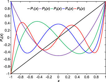
Figure 18. Legendre polynomials up to the 5th degree.
Download figure:
Standard image High-resolution image2.5.4. Bessel functions.
The nth-order Bessel function of the first kind is defined as [92]:
They relate to the Zernike radial polynomials via [32]:
which is of great importance for the reduction of the diffraction integral in the Nijboer–Zernike theory [6, 21]. The first few terms of the Bessel functions are illustrated in figure 19.

Figure 19. Bessel functions of the first kind up to the 4th degree.
Download figure:
Standard image High-resolution image2.5.5. Chebyshev polynomials.
The Chebyshev polynomials of the second kind and of degree n are defined as [51]:
They relate to the Radon transforms of Zernike radial polynomials  via [93]:
The equation (85) can be used to compute the Zernike radial polynomials for large values of the degree n [94]. The first few terms of the Chebyshev polynomials of the second kind are illustrated in figure 20.

Figure 20. Chebyshev polynomials of the second kind up to the 4th degree.
Download figure:
Standard image High-resolution image2.5.6. Pseudo Zernike polynomials.
The pseudo Zernike polynomials (see table 14), first derived by Bhatia and Wolf in 1954 [3], are a set of polynomials orthogonal over a unit circle and analogous to complex Zernike circle polynomials. They are obtained by eliminating the condition n − |l| = even from the definition of the complex Zernike circle polynomials in equation (16). Specifically, the pseudo Zernike polynomials are defined as:

Table 14. Pseudo Zernike polynomials up to the 5th degree.
| j | n | l | νj (ρ, θ) |
|---|---|---|---|
| 1 | 0 | 0 | 1 |
| 2 | 1 | −1 |

|
| 3 | 0 |

| |
| 4 | 1 |

| |
| 5 | 2 | −2 |

|
| 6 | −1 |
| |
| 7 | 0 |
| |
| 8 | 1 |
| |
| 9 | 2 |

| |
| 10 | 3 | −3 |

|
| 11 | −2 |
| |
| 12 | −1 |

| |
| 13 | 0 |
| |
| 14 | 1 |

| |
| 15 | 2 |
| |
| 16 | 3 |

| |
| 17 | 4 | −4 |

|
| 18 | −3 |
| |
| 19 | −2 |

| |
| 20 | −1 |

| |
| 21 | 0 |

| |
| 22 | 1 |

| |
| 23 | 2 |

| |
| 24 | 3 |
| |
| 25 | 4 |

| |
| 26 | 5 | −5 |

|
| 27 | −4 |

| |
| 28 | −3 |

| |
| 29 | −2 |

| |
| 30 | −1 |

| |
| 31 | 0 |

| |
| 32 | 1 |

| |
| 33 | 2 |

| |
| 34 | 3 |

| |
| 35 | 4 |
| |
| 36 | 5 |

|
where n is a nonnegative integer, l is an integer, and n − |l| ⩾ 0; the radial polynomials of pseudo Zernike polynomials can be written as:
The relation between the pseudo Zernike radial polynomials (equation (87)) and the Zernike radial polynomials (equation (19)) is given by [3]:
The first few terms of the pseudo Zernike radial polynomials are illustrated in figure 21. Pseudo Zernike polynomials can be used for wavefront sensing [83], and to define pseudo Zernike moments, which can generate moment invariants as shape descriptors for pattern recognition (section 4.6.2).

Figure 21. Pseudo Zernike radial polynomials with the azimuthal index l = 1.
Download figure:
Standard image High-resolution image3. Zernike polynomials over noncircular pupils
3.1. Zernike polynomials over arbitrary pupil shapes
Zernike circle polynomials are in widespread use for wavefront analysis in optical systems with circular pupils. They are unique in the sense that they are not only orthogonal across a unit circle, but they also represent balanced aberrations yielding minimum variance. However, in practice, optical systems do not always have circular pupil shapes. Non-circular pupils, such as annular, hexagonal, elliptical, rectangular, and square, are also very common. For example, many telescopes, such as the Hubble space telescope, have annular pupils [95, 96]; some mirrors of large telescopes are segmented into small hexagonal segments to facilitate fabrication, testing, and alignment [97]; the pupil of a human eye is slightly elliptical [98]; rectangular or square optics are applied in anamorphic optical systems [99, 100] and high-powered laser systems [101]. In such cases, Zernike circle polynomials are no longer orthogonal and their advantages are lost. It is necessary to construct new orthonormal polynomials for aberration representation. Methods for constructing orthonormal polynomials mainly include the recursive Gram–Schmidt process [37] and the nonrecursive matrix approach [102]. The Gram–Schmidt orthogonalization approach is briefly summarized below.
Using the Gram–Schmidt orthonormalization process [103], a set of polynomials Fj (x, y) orthogonal over noncircular pupils can be constructed from Zernike circle polynomials as [4, 37, 104]:
where  denotes the mean value of
  and is defined as:
where A is the area of the region of integration. Nj +1 is a normalization factor and can be expressed as:
The constructed polynomials satisfy the following orthonormality condition:
Since an orthonormal polynomial is a linear combination of Zernike circle polynomials (equation (89)), the wavefront decomposition with a set of orthonormal polynomials over noncircular pupils is identical to the decomposition with a corresponding set of Zernike circle polynomials. However, in this case, the Zernike circle polynomials do not represent balanced aberrations and their expansion coefficients lack physical significance [105].
The constructed orthogonal polynomials are determined recursively and each term is a linear combination of Zernike circle polynomials with no higher radial order. The Gram–Schmidt orthonormalization approach can be applied to construct orthonormal polynomials over any pupil shape [106, 107]. Figure 22 presents five common noncircular pupils, including annular, rectangular, square, hexagonal, and elliptical pupils. Orthonormal polynomials over these noncircular pupils can be obtained using the Gram–Schmidt orthogonalization process and are tabulated in table 15.

Figure 22. Common noncircular pupils inscribed inside a unit circle. (a) Annular pupil (obscuration ratio: ). (b) Rectangular pupil (half width: a). (c) Square pupil. (d) Hexagonal pupil. (e) Elliptical pupil (semi-minor axis: a).
Download figure:
Standard image High-resolution image
![${F_{j + 1}} = {N_{j + 1}}\left[ {{Z_{j + 1}} - \sum\limits_{i = 1}^j {\overline {{Z_{j + 1}}{F_i}} } {F_i}} \right]$](https://content.cld.iop.org/journals/2040-8986/24/12/123001/revision3/joptac9e08ieqn418.gif)
3.2. Zernike polynomials over annular pupils
Annular pupil plays an important role in optical systems, such as telescopes for astronomical observation [96] and stitching interferometers for aspheric wavefront testing by annular sub-apertures [109–111]. Orthonormal Zernike polynomials over annular pupils, called Zernike annular polynomials, can be constructed using the Gram–Schmidt orthogonalization process based on Zernike circle polynomials. Zernike annular polynomials first appeared in a report of Perkin-Elmer Corporation in 1971 [4], were later discussed by Tatian in 1976 [5] and systematically studied and explicitly given by Mahajan in 1981 [4].
Zernike annular polynomials are defined over a unit annular disk with an obscuration ratio of (0 ⩽ < 1) and can be most conveniently expressed in polar coordinates (ρ, θ), where ρ is the normalized radial coordinate ( ⩽ ρ⩽ 1) and θ is the polar angle measured counterclockwise from the +x-axis (0 ⩽ θ < 2π), as shown in figure 23.

Figure 23. Unit annular pupil with an obscuration ratio of .
Download figure:
Standard image High-resolution image3.2.1. Definition.
3.2.1.1. Real Zernike annular polynomials
Real Zernike annular polynomials have normalized and non-normalized forms. The normalized form defined under the Noll indexing scheme can be written as [4, 35, 112]:
where the index n is the degree of the radial polynomials,  ; the index m is the azimuthal frequency describing the repetition of the angular function; n and m are non-negative integers and satisfy n − m⩾ 0 and n − m= even; j is a mode-ordering number starting from 1, and is the obscuration ratio. There are a total of (n + 1)(n + 2)/2 linearly independent polynomials for a specific degree of n. The radial polynomials
  can be obtained by Gram–Schmidt orthogonalization and are given by:
where:
and the weighting factor  can be determined according to the orthogonality condition of the radial polynomials as:
Exemplary profiles of the radial polynomials are shown in figure 24. It is easy to verify that when = 0, Zernike annular polynomials reduce to circle polynomials. The normalized Zernike annular polynomials meet the following orthonormality condition:

Figure 24. Annular Zernike radial polynomials ( = 0.5) of the first few degrees when m = 0, 1, and 2.
Download figure:
Standard image High-resolution imagewhere  is the Kronecker delta function.
Similar to Zernike circle polynomials, orthonormal Zernike annular polynomials can be sorted by either the single index, j, or the double indices, n and m. The former is useful for describing Zernike expansion coefficients while the latter is useful for unambiguously describing the functions. To convert between the indices n, m, and j, one can use the relationships described in equation (8) and (9). Table 16 lists the first 28-term orthonormal real Zernike annular polynomials in the polar coordinate system and the values for n, m, and j. For more terms up to the 45th, one can refer to the tables 5–7 in [104].
Table 16. Zernike annular polynomials under the Noll indices up to the sixth degree (n = 6).
| j | n | m |

|

| Aberration |
|---|---|---|---|---|---|
| 1 | 0 | 0 | 1 |

| Piston |
| 2 | 1 | 1 |

|

| X Tilt |
| 3 | 1 |

| Y Tilt | ||
| 4 | 2 | 0 |

|

| Defocus |
| 5 | 2 |

|
| Primary Y astigmatism | |
| 6 | 2 |
| Primary X astigmatism | ||
| 7 | 3 | 1 |
![$\frac{{3(1 + {\varepsilon ^2}){\rho ^3} - 2(1 + {\varepsilon ^2} + {\varepsilon ^4})\rho }}{{(1 - {\varepsilon ^2}){{[(1 + {\varepsilon ^2})(1 + 4{\varepsilon ^2} + {\varepsilon ^4})]}^{1/2}}}}$](https://content.cld.iop.org/journals/2040-8986/24/12/123001/revision3/joptac9e08ieqn441.gif)
|
| Primary Y coma |
| 8 | 1 |
| Primary X coma | ||
| 9 | 3 |

|
| ||
| 10 | 3 |
| |||
| 11 | 4 | 0 |
![$\frac{{[6{\rho ^4} - 6(1 + {\varepsilon ^2}){\rho ^2} + 1 + 4{\varepsilon ^2} + {\varepsilon ^4}]}}{{{{(1 - {\varepsilon ^2})}^2}}}$](https://content.cld.iop.org/journals/2040-8986/24/12/123001/revision3/joptac9e08ieqn447.gif)
|

| Primary spherical |
| 12 | 2 |
![$\frac{{4{\rho ^4} - 3[(1 - {\varepsilon ^8})/(1 - {\varepsilon ^6})]{\rho ^2}}}{{{{\left\{ {{{(1 - {\varepsilon ^2})}^{ - 1}}\left[ {16(1 - {\varepsilon ^{10}}) - 15{{(1 - {\varepsilon ^8})}^2}/(1 - {\varepsilon ^6})} \right]} \right\}}^{1/2}}}}$](https://content.cld.iop.org/journals/2040-8986/24/12/123001/revision3/joptac9e08ieqn449.gif)
|
| Secondary X astigmatism | |
| 13 | 2 |
| Secondary Y astigmatism | ||
| 14 | 4 |
|
| ||
| 15 | 4 |
| |||
| 16 | 5 | 1 |
![$\frac{{\left[ 10(1 + 4{\varepsilon ^2} + {\varepsilon ^4}){\rho ^5} - 12(1 + 4{\varepsilon ^2} + 4{\varepsilon ^4} + {\varepsilon ^6}){\rho ^3} + 3(1 + 4{\varepsilon ^2} + 10{\varepsilon ^4} + 4{\varepsilon ^6} + {\varepsilon ^8})\rho \right]}}{{{{(1 - {\varepsilon ^2})}^2}{{[(1 + 4{\varepsilon ^2} + {\varepsilon ^4})(1 + 9{\varepsilon ^2} + 9{\varepsilon ^4} + {\varepsilon ^6})]}^{1/2}}}}$](https://content.cld.iop.org/journals/2040-8986/24/12/123001/revision3/joptac9e08ieqn455.gif)
|
| Secondary X coma |
| 17 | 1 |

| Secondary Y coma | ||
| 18 | 3 |
![$\frac{{5{\rho ^5} - 4[(1 - {\varepsilon ^{10}})/(1 - {\varepsilon ^8})]{\rho ^3}}}{{{{\left\{ {{{(1 - {\varepsilon ^2})}^{ - 1}}[25(1 - {\varepsilon ^{12}}) - 24{{(1 - {\varepsilon ^{10}})}^2}/(1 - {\varepsilon ^8})]} \right\}}^{1/2}}}}$](https://content.cld.iop.org/journals/2040-8986/24/12/123001/revision3/joptac9e08ieqn458.gif)
|
| ||
| 19 | 3 |
| |||
| 20 | 5 |
|
| ||
| 21 | 5 |
| |||
| 22 | 6 | 0 |
![$\frac{{[20{\rho ^6} - 30(1 + {\varepsilon ^2}){\rho ^4} + 12(1 + 3{\varepsilon ^2} + {\varepsilon ^4}){\rho ^2} - (1 + 9{\varepsilon ^2} + 9{\varepsilon ^4} + {\varepsilon ^6})]}}{{{{(1 - {\varepsilon ^2})}^3}}}$](https://content.cld.iop.org/journals/2040-8986/24/12/123001/revision3/joptac9e08ieqn464.gif)
|

| Secondary spherical |
| 23 | 2 |
![$\scriptsize{\frac{{\left[ \begin{array}{l} 15(1 + 4{\varepsilon ^2} + 10{\varepsilon ^4} + 4{\varepsilon ^6} + {\varepsilon ^8}){\rho ^6} - 20(1 + 4{\varepsilon ^2} + 10{\varepsilon ^4} + 10{\varepsilon ^6} + 4{\varepsilon ^8} \\ + {\varepsilon ^{10}}){\rho ^4} + 6(1 + 4{\varepsilon ^2} + 10{\varepsilon ^4} + 20{\varepsilon ^6} + 10{\varepsilon ^8} + 4{\varepsilon ^{10}} + {\varepsilon ^{12}}){\rho ^2} \\ \end{array} \right]}}{{\left\{ {{{(1 - {\varepsilon ^2})}^2}{{\left[ \begin{array}{l} (1 + 4{\varepsilon ^2} + 10{\varepsilon ^4} + 4{\varepsilon ^6} + {\varepsilon ^8})(1 + 9{\varepsilon ^2} + 45{\varepsilon ^4} \\ + 65{\varepsilon ^{\text{6}}} + 45{\varepsilon ^8} + 9{\varepsilon ^{10}} + {\varepsilon ^{12}}) \\ \end{array} \right]}^{1/2}}} \right\}}}}$](https://content.cld.iop.org/journals/2040-8986/24/12/123001/revision3/joptac9e08ieqn466.gif)
|
| Tertiary Y astigmatism | |
| 24 | 2 |
| Tertiary X astigmatism | ||
| 25 | 4 |
![$\frac{{6{\rho ^6} - 5[(1 - {\varepsilon ^{12}})/(1 - {\varepsilon ^{10}})]{\rho ^4}}}{{{{\left\{ {{{(1 - {\varepsilon ^2})}^{ - 1}}[36(1 - {\varepsilon ^{14}}) - 35{{(1 - {\varepsilon ^{12}})}^2}/(1 - {\varepsilon ^{10}})]} \right\}}^{1/2}}}}$](https://content.cld.iop.org/journals/2040-8986/24/12/123001/revision3/joptac9e08ieqn469.gif)
|
| ||
| 26 | 4 |
| |||
| 27 | 6 |
|

| ||
| 28 | 6 |

|
The non-normalized Zernike annular polynomials can be obtained by dropping the normalization factors from the orthonormal Zernike annular polynomials as:
They satisfy the following orthogonality condition:
Figures 25 and 26 show the 3D visualization of the non-normalized Zernike annular polynomials up to the sixth degree for = 0.6 and their corresponding interferometric fringe patterns as in optical testing [37].

Figure 25. Pyramid of the non-normalized Zernike annular polynomials up to the sixth degree with an obstruction ratio of 0.6.
Download figure:
Standard image High-resolution image
Figure 26. Interferometric fringe patterns of the Zernike annular aberrations shown in figure 25.
Download figure:
Standard image High-resolution image3.2.1.2. Complex Zernike annular polynomials
Complex Zernike annular polynomials have normalized and non-normalized forms. The normalized complex Zernike annular polynomials defined in the Noll indices can be written as [4, 35]:

where n is a non-negative integer, l is an integer, n − |l| ⩾ 0 and is even, and the radial polynomial is defined as:
and the weighting factor  is given by:
The normalized complex Zernike annular polynomials satisfy the following orthonormality condition:
The non-normalized complex Zernike annular polynomials can be written as:

They satisfy the following orthogonality condition:
3.2.1.3. Summary.
The definitions for the real and complex Zernike annular polynomials are summarized in table 17.
Table 17. Summary of the definition of Zernike annular polynomials.
| Real Zernike annular polynomials | Complex Zernike annular polynomials | |
|---|---|---|
| Sources | Tatian, 1974 [5] Mahajan, 1981 [4] Zemax [25] | Mahajan, 1981 [4] |
| Indexing | The Noll indices | The Noll indices |
| Definition |
![$\begin{array}{l} {Z_j}(\rho ,\theta ;\varepsilon ) = Z_n^m(\rho ,\theta ;\varepsilon ) \\[4pt] = N_n^m\left\{ {\begin{array}{*{20}{l}} {R_n^m(\rho ;\varepsilon )\cos m\theta ,}\;{m \ne 0, \;j {\text{ is even}}} \\[4pt] {R_n^m(\rho ;\varepsilon )\sin m\theta ,}\;\;{m \ne 0,\; j {\text{ is odd}}} \\[4pt] {R_n^m(\rho ;\varepsilon ),}\;\qquad \quad {m = 0} \end{array} } \right. \\ \end{array} $](https://content.cld.iop.org/journals/2040-8986/24/12/123001/revision3/joptac9e08ieqn476.gif)
|

|
| Radial polynomials | Equation (94) | Equation (101) |
| Coordinate system | 0 ⩽ ρ ⩽ 1 θ from +x axis anticlockwise | 0 ⩽ ρ ⩽ 1 θ from +x axis anticlockwise |
| Normalization | Optional | Optional |
| Normalization factor |
![$N_n^m = \left\{ \begin{array}{l} 1,\;\;\;\;\;\;\;\;\;\;\;\;\;\;{\text{non-normalized}} \\[6pt] \sqrt {\frac{{2(n + 1)}}{{(1 + {\delta _{m0}})}}} ,\;{\text{normalized}} \\ \end{array} \right.$](https://content.cld.iop.org/journals/2040-8986/24/12/123001/revision3/joptac9e08ieqn478.gif)
|
![$N_n^l = \left\{ \begin{array}{l} 1,\;\;\;\;\;\;\;\;{\text{non-normalized}} \\[6pt] \sqrt {n + 1} ,\;{\text{normalized}} \\ \end{array} \right.$](https://content.cld.iop.org/journals/2040-8986/24/12/123001/revision3/joptac9e08ieqn479.gif)
|
| Term number | Infinite | Infinite |
| Indices | j = 1, 2, 3, ..., ∞ n: non-negative integer m: non-negative integer n − m ⩾ 0 and even | n: non-negative integer l: integer n − |l| ⩾ 0 and even |
| Relationship between indices |
![$j = \left\{ {\begin{array}{*{20}{l}} {\frac{{n(n + 1)}}{2} + 1,}&{m = 0} \\[6pt] {\left[ {\frac{{n(n + 1)}}{2} + m,\frac{{n(n + 1)}}{2} + m + 1} \right],}&{m \ne 0} \end{array}} \right.$](https://content.cld.iop.org/journals/2040-8986/24/12/123001/revision3/joptac9e08ieqn480.gif)
![$\begin{array}{l} n = \left\lfloor {\left( {\sqrt {2j - 1} + 0.5} \right) - 1} \right\rfloor \\[8pt] m = \left\{ {\begin{array}{*{20}{l}} {2 \times \left\lfloor {\frac{{2j + 1 - n\left( {n + 1} \right)}}{4}} \right\rfloor ,}&{n{\text{ is even}}} \\[8pt] {2 \times \left\lfloor {\frac{{2\left( {j + 1} \right) - n\left( {n + 1} \right)}}{4}} \right\rfloor - 1,}&{n{\text{ is odd}}} \end{array}} \right. \\ \end{array} $](https://content.cld.iop.org/journals/2040-8986/24/12/123001/revision3/joptac9e08ieqn481.gif)
| — |
| Ordering | n, m both in ascending order | — |
3.2.2. Mathematical properties.
3.2.2.1. Orthogonality.
The orthogonal relationships of real and complex Zernike annular polynomials have been presented and can be found in equations (97), (99), (103) and (105). Moreover, the radial polynomials of Zernike annular polynomials are also orthogonal over the annular aperture and satisfy the following relationships [4]:
3.2.2.2. Recurrence relation.
The recurrence relationship for generating radial polynomials of Zernike annular polynomials was derived by Tatian in 1974 [4, 5] and can be written as:
where n and m obey the same conditions defined in Zernike annular polynomials (n and m are non-negative integers, n − m⩾ 0 and is even); k is a non-negative integer (k = 0, 1, 2, ..., ∞); l = (n − m)/2; u = ρ2;  is a set of orthogonal polynomials obtained by orthogonalizing the sequence 1, u, ..., ul
over the interval (2, 1) with a weight function um
and can be written as [4, 5]:
is a set of orthogonal polynomials obtained by orthogonalizing the sequence 1, u, ..., ul
over the interval (2, 1) with a weight function um
and can be written as [4, 5]:
The coefficient  is:
is:
Especially, when m = n,
The above recurrence relationship can be initialized with  .
.
3.2.2.3. The Fourier transform.
The Fourier transform of Zernike annular polynomials is derived by Dai and Mahajan [95] and can be written as:
where (r, φ) denotes the polar coordinates in the frequency domain and:
where J is the Bessel function of the first kind (equation (82)) and:
A list of the first few terms for  ,
,  , and
, and  can be found in [95]. The expression in equation (111) reduces to the Fourier transform of Zernike circle polynomials (equation (30)) when = 0.
3.2.3. Wavefront fitting.
The orthogonality of Zernike annular polynomials makes them an excellent basis for wavefront analysis in annular optical systems. An annular wavefront can be represented by the linear combination of finite terms of Zernike annular polynomials as [113]:
where J is the total terms of the polynomials, aj is the expansion coefficients, and Zj is the jth-term Zernike annular polynomial. The equation can be equivalently expressed in Cartesian coordinates as:
Written in discrete and matrix forms, equation (51) becomes:

where:
where K is the total number of data points within the unit circle. Generally, equation (117) is an overdetermined linear system, where there are more equations (K) than unknowns (J). It can be written into the normal equation [34, 68]:

where the superscript T denotes matrix transpose. The solution can be obtained by matrix inversion as:

Figure 27 shows an example illustrating annular wavefront decomposition using 28-term orthonormal Zernike annular polynomials under the Noll indices. The amplitude of each coefficient indicates the strength of corresponding aberrations (table 16).

Figure 27. Annular wavefront decomposition using orthonormal Zernike annular polynomials under the Noll indices: (a) wavefront and (b) 28 expansion coefficients.
Download figure:
Standard image High-resolution image4. Applications
The unique properties of Zernike polynomials have enabled them to be an attractive mathematical tool in many fields. In this section, we survey their applications in a range of fields, including diffraction theory, optical design, optical testing, adaptive optics, ophthalmic optics, and image analysis, as illustrated in figure 28.

Figure 28. Major applications of Zernike polynomials.
Download figure:
Standard image High-resolution image4.1. Diffraction theory
4.1.1. The diffraction theory of aberrations.
Zernike polynomials have important applications in the diffraction theory of aberrations, which is concerned with the study of how wavefront aberrations affect image formation in practical optical systems [32, 47]. In a perfect optical imaging system, the light waves from a point object emerge in the image space as spherically convergent waves and form the well-known Airy pattern. However, a perfect imaging system never exists in practice. Waves emerging from a practical optical system deviate from a spherical wave and possess complicated forms.
Consider the wave propagation model illustrated in figure 29, where an aberrated wavefront at the exit pupil converges to the image plane. Let Wa and Wr denote the aberrated wavefront and its Gaussian reference wavefront in the unit of length, respectively. The position of the exit pupil is defined by the Cartesian coordinates (x, y, z) or the cylindrical coordinates (ρ, θ, z); the position of the image plane is defined by the Cartesian coordinates (ξ, η, ζ) or the cylindrical coordinates (r, φ, υ). The complex amplitude distribution at the exit pupil, called the pupil function, can be written as [114]:


Figure 29. Geometry of wave propagation from the exit pupil to the image plane. Wa: aberrated wavefront; Wr: reference wavefront.
Download figure:
Standard image High-resolution imagewhere A(ρ, θ) is the amplitude function and Φ is the phase function in the form of:
where λ is the wavelength. According to the scalar Debye integral [32, 114], the normalized complex amplitude, U(r, φ, υ), in the focal region of the image plane is given by:
where υ is defined as the negative axial coordinate (-ζ) normalized with respect to the axial diffraction unit,  , and s0 is the numerical aperture (NA) of the focusing beam. When the image plane is at the best focus (υ = 0), the complex amplitude U(r, φ, υ) in equation (123) reduces to the Fourier transform of the pupil function P(ρ, θ).
The PSF, defined as the diffraction pattern of a point object in the image plane, can be written as the squared modulus of the complex amplitude U [115, 116], i.e.

The image of an extended object formed by an optical system is the convolution of the object itself with the PSF of the system, which can be mathematically modeled as [117]:

where f and g denote the object and the image, respectively, and ∗ represents convolution. To understand the impact of wavefront aberrations on the final image quality, the PSF needs to be evaluated. In the next section, we briefly review the analytical PSF computation approaches first developed by Nijboer and Zernike [6, 21] and later extended by Janssen [8], where expanding wavefront aberrations at the exit pupil using Zernike circle polynomials is the key.
4.1.2. PSF computation using the Nijboer–Zernike theory.
In general, analytical evaluation of the diffraction integrals in equation (123) is difficult except for some specific cases. In 1942, Bernard Nijboer, a PhD, student of Zernike, expanded the aberration function at the exit pupil into a series of Zernike circle polynomials and formulated an efficient representation of the complex amplitude distribution in the image plane [6, 21]. This work allows analytical evaluation of the diffraction integral and the PSF of a general optical system and is referred to as the Nijboer–Zernike theory. For completeness, we briefly review the basic principle of the theory, which is well summarized in [114].
In the Nijboer–Zernike theory, the pupil function is assumed to be uniform in amplitude and thus can be written as a purely phase-aberrated function, i.e.

Expanding the pupil function into the Taylor series, the diffraction integral in equation (123) becomes:
Expanding the phase function, Φ(ρ, θ), into a set of Zernike circle polynomials gives:
Substituting the Zernike expansion into the integral (equation (127)) and performing the integration over θ using elementary Bessel function operations, we obtain:
where  is the Zernike expansion coefficients and Jm
is a Bessel function of the first kind and of order m. Note that in the reduction, the phase aberration is considered small enough so that truncation of the infinite series in equation (128) after the term k = 1 is allowed. The above equation can be further reduced using the relationship in equation (83) as:
is the Zernike expansion coefficients and Jm
is a Bessel function of the first kind and of order m. Note that in the reduction, the phase aberration is considered small enough so that truncation of the infinite series in equation (128) after the term k = 1 is allowed. The above equation can be further reduced using the relationship in equation (83) as:
where the prime indicating that m = n = 0 should be excluded from the summation.
The expression of the complex amplitude, U, provides an analytical method for evaluating the PSF of an optical system. Although elegant in expression, the Nijboer–Zernike approach is not widely used in practice [114], largely because that the derivation requires the amplitude over the pupil to be uniform and the wavefront aberration is restricted to be sufficiently small (in the order of a fraction of the wavelength [32]).
Figure 30 illustrates the appearance of the PSF of an optical system when only a single Zernike term (root mean square value: 0.1 μm, wavelength: 570 nm) is present in the wavefront aberration. Figure 31 presents an example showing that wavefront aberrations degrade the image quality of an optical system.

Figure 30. PSFs of the Zernike circle polynomials (root mean square value: 0.1 μm) up to the fourth degree under the Noll indices.
Download figure:
Standard image High-resolution image
Figure 31. Convolution of an object with the PSF of an optical system leads to degraded images.
Download figure:
Standard image High-resolution image4.1.3. PSF computation using the extended Nijboer–Zernike theory.
The Nijboer–Zernike theory is only valid in the case of small aberrations and can only produce accurate values of PSF at positions close to geometrical focus. To deal with the problem, Janssen in 2002 formulated a general expression in terms of the power-Bessel series and extended the Nijboer–Zernike theory for optical systems with large aberrations [8, 114, 118, 119]. The extended Nijboer–Zernike theory can analytically compute the PSF of an aberrated optical system described by Zernike coefficients and accelerates further developments in focused field diffraction theory.
The extended Nijboer–Zernike theory adopts a generalized definition for the pupil function and expands it using Zernike circle polynomials as [114]:

where the amplitude, A(ρ, θ), and phase aberration, Φ(ρ, θ), are real-valued; the coefficients,  , is in general complex-valued;
  is the non-normalized complex Zernike circle polynomials defined in equation (16). Substituting the pupil function into the diffraction integral (equation (123)), the complex amplitude, U, can be expressed as:
where:
Janssen derived a Bessel series representation for the integral in equation (133) and reformulate the above equation as:
where:
The symbol  denotes combination and is defined as:
Note that the equation (134) suffers from loss-of-digits and slow convergence for larger υ under standard precision. An advanced version of the ENZ-theory has been developed to virtually eliminate the convergence problem by replacing the power-Bessel series in equation (134) with Bessel-Bessel series [120]. Using equation (134), we can compute the PSF of an optical system with an exit pupil defined by a set of β-coefficients (equation (131)). The extended Nijboer–Zernike theory has been used in several applications, such as aberration retrieval in high-NA optical lithography systems [121–123] and acoustic diffraction problems [124, 125].
4.2. Optical design
Optical design is the process of designing an optical system to meet specific performance requirements and constraints. Owing to their unique properties, Zernike polynomials are beneficial to wavefront analysis and surface representation in modern lens design programs. In wavefront analysis, since Zernike expansion coefficients are independent and directly represent balanced aberrations, it is convenient to decompose wavefront aberrations of an optical system into a set of Zernike polynomials to evaluate the contribution of each aberration [25]. Moreover, the coefficients of Zernike polynomials can also be used as variables of the merit function of a lens system to facilitate system optimization [126].
In surface representation, Zernike polynomials have emerged as a means of describing the shape of freeform optical surfaces [127–131]. State-of-the-art lens design programs, such as Zemax and CODE V, empower optical designers to use Zernike polynomials to represent freeform surfaces, which are called Zernike surfaces. For example, Zernike phase surfaces and Zernike sag surfaces are defined and used in Zemax. The Zernike phase surfaces are standard surfaces, such as planes, spheres, and conics, superimposed with phase terms defined by Zernike polynomials [132]. The phase term can be written as:
where m represents the diffraction order, Zj is Zernike circle polynomials, and aj is the expansion coefficients, ρ is the normalized radial coordinate and θ is the polar angle. This surface type is well suited to modeling system aberrations for which measured interferometer data is available [132]. The Zernike sag surfaces are defined as the conic surface (figure 32) plus additional deformation terms characterized by even orders of the power series and finite terms of Zernike polynomials [58, 132]. They are given by:
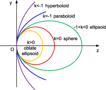
Figure 32. Conic surfaces.
Download figure:
Standard image High-resolution imagewhere c denotes the curvature of the base conic; r = x2 + y2 is the radial ray coordinate in lens unit; k is the conic constant; αj and aj are the coefficients of the power series and the Zernike polynomials, respectively; J is the maximum number of terms of the Zernike polynomials; ρ is the normalized radial coordinate and θ is the polar angle. The Zernike phase surfaces (equation (138)) describe phase variation of a surface while the Zernike sag surfaces (equation (139)) characterize surface deformations. These Zernike surfaces can also employ Zernike annular polynomials to define the aspheric terms when an optical system has an annular pupil. Figure 33 is an example showing the design of a long wave infrared reflective imaging system optimized with Zernike surfaces [133].

Figure 33. Optical system design with Zernike polynomials. (a) Optical layout of a long wave infrared reflective imaging system optimized with Zernike surfaces. (b) Housing structure of the optical system. Reprinted with permission from [133] © The optical Society.
Download figure:
Standard image High-resolution image4.3. Optical testing
Optical testing is concerned with testing the optical quality of optical systems by optical techniques [134, 135]. The applications of Zernike polynomials in optical testing are mainly concentrated in the field of optical surface or wavefront measurement by phase-shifting interferometry [136], the principal purpose of which is to determine the aberrations present in an optical component or an optical system [19]. There are many different types of phase-shifting interferometers used in practice, such as the Fizeau, Mach-Zehnder, and Twyman-Green interferometers [137–140]. Here we use a phase-shifting Twyman-Green interferometer as an example to demonstrate the usefulness of Zernike polynomials in precise surface figure measurement.
A typical optical layout of a phase-shifting Twyman-Green interferometer is shown in figure 34. The emitted beam from a laser source is first collimated by a beam expander and then divided by a beam splitter into two parts. The reflected part (red) propagates to a reference mirror and is then reflected back serving as the reference beam. The transmitted part (blue), after passing through a compensation lens, is incident onto the optical surface under test and then reflected back along the same path. The reference beam and the measurement beam meet at the beam splitter, interfere with each other, and produce fringe patterns with periodic intensity modulation. The fringe patterns carry the surface figure information of the optical component under test and are finally recorded by a charge-coupled device (CCD) detector. Phase shifting is achieved by moving the reference mirror a certain amount with a piezoelectric transducer (PZT).

Figure 34. A phase-shifting Twyman-Green interferometer for optical surface testing. PZT: piezoelectric transducer. CCD: charge-coupled device. Adapted with permission from [141] © The optical Society.
Download figure:
Standard image High-resolution imageThe intensity of a fringe pattern can be mathematically modeled as [142–144]:

where a(x, y) and b(x, y) are the background and the modulation terms, respectively, and Φ(x, y) is the phase map to be recovered. There are three unknowns in equation (140), indicating at least three frames of phase-shifted interferograms are needed to recover the phase function. This is known as the three-step or three-bucket phase demodulation algorithm. In practice, there are many more different phase-shifting algorithms in use, such as the four-step, five-step, and least- squares algorithms [137, 138, 142]. Herein the four-step algorithm will be introduced. Suppose that four interferograms with phase shifts of 0, π/2, π, and 3π/2 are collected. Their intensity functions can be written as:
The phase, Φ(x, y), can be simply calculated as:
Since the value of the inverse tangent function is within [−π, π], the calculated phase, Φ(x, y), is typically wrapped. An extra process, called phase unwrapping [145, 146], is needed to yield a continuous phase map.
Generally, misalignment errors, such as tilt and defocus, are present in the phase function, Φ(x, y) and need to be removed to reveal the true surface figure. This can be achieved by expanding the phase function into finite terms of Zernike polynomials and eliminating the coefficients of the tilt and defocus terms. Mathematically, the phase expansion can be written as:
where aj is the expansion coefficients and can be computed by the least-squares method described in section 2.3.1. The final figure map of the surface under test can be obtained as [141, 147]:

where a0, a1, a2, and a3 represent the coefficients of the piston, x-tilt, y-tilt, and defocus terms of the Zernike expansion, respectively. The Zernike expansion coefficients, aj , can be further used to calculate the PVr (peak-to-valley robust) [148], which is a robust amplitude parameter for describing the figure error of the optical surface under test.
For ease of understanding, the whole procedure for surface figure retrieval from a set of phase-shifted fringe patterns is illustrated in figure 35 and a state-of-the-art commercial Fizeau interferometer for optical testing is shown in figure 36.

Figure 35. Surface figure retrieval from a set of phase-shifted fringe patterns. (a) Phase-shifted interferograms. (b) Demodulated phase. (c) Unwrapped continuous phase. (d) 37 expansion coefficients of the Zernike circle polynomials under the fringe indices. (e) Recovered surface figure. λ: wavelength.
Download figure:
Standard image High-resolution image
Figure 36. A commercial laser Fizeau interferometer for optical surface testing. Reproduced with permission from Zygo Corporation. ©2021 Zygo Corporation.
Download figure:
Standard image High-resolution image4.4. Ophthalmic optics
The eye, like any other optical system, suffers from a number of specific optical aberrations [149]. Aberrations of eyes with refractive errors include lower-order aberrations and higher-order aberrations. Lower-order aberrations, such as myopia, hyperopia, and regular astigmatism, account for approximately 90% of the overall ocular aberration and are the most common causes of visual impairment [150]. In contrast, higher-order aberrations, such as spherical aberration, coma, and trefoil, account for less than 10% of ocular aberrations but they may significantly impact on visual performance when the pupil is large [149, 151]. Measuring the aberrations of the human eye can provide objective and quantitative data for vision correction and is of critical importance to certain corrective measures [23, 152], such as wavefront-guided refractive surgery [153, 154], which has been a paradigm shift in the field of refractive error correction. The most commonly used tool for the measurement of ocular aberrations is the Shack–Hartmann wavefront slope sensor [155], which was developed by Shack and Platt in the late 1960s [156, 157] and is an evolutionary technology of the Hartmann Screen test. The Shack–Hartmann wavefront slope sensor can measure wavefront like an interferometer but uses optical components less expensive.
The setup and principle for aberrations measurement of the eye using a Shack–Hartmann wavefront slope sensor are illustrated in figure 37. An incident infrared light beam is reflected by a beam splitter and focused onto the retina. Since the beam diameter is small (approximately 1 mm), the light spot on the retina can be regarded as a point source independent of eye aberrations. This point source emits spherical waves, which will be affected by eye aberrations and become aberrated planar waves when leaving the eye. The aberrated waves pass through the beam splitter and are detected by a Shack–Hartmann wavefront slope sensor, which consists of a 2D microlens array and a CCD camera located at the focal plane of the microlenses. In this arrangement, the whole aberrated wavefront is actually divided into many smallareas, which can be locally treated as plane waves and are individually focused onto the CCD camera. When the eye is aberration-free, the outgoing wavefront from the eye is planar and the CCD camera detects a regular spot pattern (shown as black dots in figure 37(b)). In contrast, when the eye has aberrations, the outgoing wavefront from the eye is aberrated and individual parts of the wavefront are tilted with respect to the reference wavefront, resulting in displaced focal spots (shown as red dots in figure 37(b)) after being imaged onto the CCD camera. The magnitude of the position shifts of the displaced spots reflects the tilt amount of the measured wavefront and can be used to recover the original wavefront using the algorithm described below.

Figure 37. Measurement of ocular wavefront aberration with a Shack–Hartmann wavefront slope sensor. (a) Setup schematic. (b) Principle of Shack–Hartmann wavefront sensing. Aberrated wavefront passing through the lenslet array is focused on a CCD. f: focal length of the lenslet array; Δx and Δy: shift of the actual spot with respect to the ideal spot in the x and y directions, respectively.
Download figure:
Standard image High-resolution imageIn a Shack–Harmann wavefront slope sensor, the relationship between the position shift of an actual spot and the slope of an aberrated wavefront can be written as [22, 23]:
where f is the focal length of the microlens array; Δx and Δy denote the shifts of the actual spot with respect to its ideal position in the x and y directions, respectively. Based on these relationships, the aberrated wavefront, W(x, y), can be recovered using either zonal or modal algorithms [22, 24]. In a modal reconstruction, the wavefront is represented by finite terms of Zernike circle polynomials as:
where aj is the expansion coefficients. Taking the derivatives with respect to x and y for both side of equation (146) at each sampling points gives [23]:
where K is the total number of sampling points. Substituting equation (145) into equation (147) yields a matrix equation as:

where:

s is a 2 K× 1 column vector containing measured wavefront slope data, a is a J× 1 column vector containing the unknown Zernike expansion coefficients, A is a 2 K× J coefficient matrix whose elements can be computed using the derivative formulas of Zernike polynomials in equation (42). The unknown a can be computed by matrix inversion as:

Substituting the expansion coefficients (equation (152)) into equation (146) gives the wavefront aberrations of the eye. The first measurement of ocular aberration using a Shack–Hartmann wavefront slope sensor was performed by Liang et al in 1994 [23]. The wavefront sensor was later improved by increasing sampling density to provide more complete descriptions of the aberrations of the eye, including irregular and classical aberrations [152]. Since then, measuring ocular aberrations by Shack–Hartmann wavefront slope sensor has become common in clinical practice. Ocular aberrations can also be measured by a wavefront curvature sensor, in which curvature polynomials can be used to obtain Zernike aberration coefficients [158].
In addition to wavefront reconstruction in a Shack–Hartmann wavefront slope sensor, Zernike polynomials are also very useful in the analysis of the aberrations of the eye [159]. Since Zernike polynomials are orthogonal over a circular disk, their expansion coefficients contain a wealth of measurable metrics, such as root mean square error, equivalent defocus, spherocylindric refraction values [155] can be derived for more illustrative description of eye aberrations. Consensus recommendations on definitions, conventions, and standards of Zernike polynomials were developed by OSA in 1999 for reporting of optical aberrations of the human eye [27]. The recommendations were later standardized in ANSI Z80.28 [14] and ISO 24157 [15, 17] and accepted by the vision community.
Figure 38 shows a photograph of a commercially available aberrometer, which uses a Shack–Hartmann wavefront slope sensor for aberrations measurement. Zernike polynomials are used for wavefront reconstruction and aberration reporting of the eye [155].
Figure 38. Photograph of a commercially available aberrometer that uses a Shack–Hartmann wavefront slope sensor. Left: Photograph of ZEISS i.Profiler. Right: interface of its analysis software. Reproduced with permission from © ZEISS.
Download figure:
Standard image High-resolution image4.5. Adaptive optics
Ground-based telescope is an important tool to explore the universe. Its image quality is critical to astronomical observations but can be degraded significantly by atmospheric turbulence-induced optical aberrations. Naturally, light coming from distant stars is plane waves before reaching the atmosphere of the earth and can theoretically form images limited only by the optical diffraction limit. However, due to the effect of atmospheric turbulence, the light wavefront will be distorted when propagating through the atmosphere, degrading the image quality of a telescope. Adaptive optics is such a technology that can improve the performance of an astronomical telescope by compensating wavefront aberrations induced by atmospheric turbulence using wavefront correctors [160, 161]. The technique was first envisioned by Babcock in 1953 [162] but did not come into common usage until the 1990s.
A typical adaptive optics system for an astronomical telescope consists of three principal subsystems: a wavefront sensor, a deformable mirror, and a control computer [163], as illustrated in figure 39. Its working principle is sketched in figure 40 and can be understood as follows. A telescope captures the light from the object of interest, such as a distant star or a satellite. Before being focused on the camera, the light is first sampled by a wavefront sensor, such as a Shack–Hartmann wavefront sensor, and the sampling data are transferred to a control computer. The control computer performs mathematical reconstruction to recover the wavefront distortion of the sampled light and drives a servo system to control the wavefront corrector, such as a deformable mirror, to compensate for the wavefront distortion. After compensation, the wavefront of the light should be less distorted, yielding images with improved quality at the camera. If the light from the object is too faint to determine the wavefront distortion, reference sources, such as nearby natural guide stars or artificial guide stars, can be used to facilitate the correction process. Figure 41 is an example showing that adaptive optics can improve the image quality of a telescope significantly.

Figure 39. Schematic of an astronomical telescope equipped with an adaptive optics system, which contains a deformable mirror, a wavefront sensor, and a control computer. Reproduced with permission from [163].
Download figure:
Standard image High-resolution image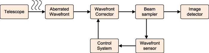
Figure 40. Working principle of adaptive optics.
Download figure:
Standard image High-resolution image
Figure 41. Adaptive optics sharpens a telescope's view. (a) No adaptive optics. (b) With adaptive optics. AO: adaptive optics. Reproduced from [164], with permission from Springer Nature.
Download figure:
Standard image High-resolution imageThe use of Zernike polynomials in adaptive optics can be reflected in two aspects. On one hand, Zernike polynomials provide a unique set of functions for the representation, reconstruction, and analysis of wavefront distortions in adaptive optics. Generally, atmospheric turbulence, described by the Kolmogorov model [160], generates smoothly varying optical wavefronts [161], which can be decomposed into different modes by Zernike polynomials [9, 161]. The decomposition makes it possible to use modal algorithms to reconstruct and analyze wavefronts measured by slope-sensitive wavefront sensors, such as the Shack-Harmann wavefront slope sensor described in section 4.4. On the other hand, Zernike polynomials offer a modal basis for the compensation of wavefront distortions caused by atmospheric turbulence. In practice, both zonal and modal approaches are used for wavefront compensation in adaptive optics [161]. The zonal approach achieves the compensation by an array of independent subapertures while the modal approach compensates for distorted wavefronts over the whole aperture. High-order aberrations are suitable for the use of the zonal method while low-order aberrations described can be compensated for more effectively by Zernike based modal methods. Although Zernike polynomials are not statistically orthogonal and are not independent [161] when used for turbulence compensation, they are near optimum for low-order corrections [9, 161, 165].
To date, adaptive optics has become a standard instrumentation suite and is in widespread use in a range of biomedical and industrial applications, such as retinal imaging [166–168], optical microscopy [169–172], optical tweezer [173], micro/nanofabrication [174–176], and optical storage [177]. Figure 42 shows representative applications of adaptive optics in laser fabrication, optical coherence tomography (OCT), and super-resolution microscopy with improved performance.

Figure 42. Applications of adaptive optics in industry and biomedicine. (a) Ultrafast laser fabrication beneath the surface of diamond without and with aberration correction. Adapted with permission from [174] © The optical Society. (b) Ultrafast laser writing of structures in glasses without and with wavefront correction. Adapted with permission from [175] © The optical Society (c) In vivo OCT tomograms of a normal human eye in the foveal region without and with adaptive optics. Adapted with permission from [178] © The optical Society. (d) Mitochondria (magenta) and the plasma membrane (green) in a cell ∼150 μm deep in a zebrafish hindbrain imaged without and with aberration correction and deconvolution. Reproduced from [172], with permission from Springer Nature.
Download figure:
Standard image High-resolution image4.6. Image analysis
In addition to applications in optics, Zernike polynomials also play an important role in moments-based image analysis. Image moments are real- or complex-valued quantities used to characterize an image function and describe its features. They are commonly used in statistics to characterize the distribution of random variables and in mechanics to measure the mass distribution of a body. The use of moments for image analysis is straightforward if we treat the pixel intensity of a binary or gray level image as a random variable. Image moments, M, can be considered as projections of an image function onto a set of basis functions and are mathematically defined as:
where f(x, y) is the image function and ψ(x, y) is the basis function.
Image moments have been intensively studied in image analysis because they can be used to construct moment invariant features for the description and recognition of deformed objects and patterns. Common moments used for image analysis include geometric moments, rotational moments, complex moments, and orthogonal moments [48, 179]. Among them, geometric moments, which use a power series as the basis function [ψ(x, y) = xnyl ], are the earliest. Based on geometric moments, Hu first introduced moment invariants in 1962 using the theory of algebraic invariants and constructed seven moment invariants to linear transformations (translation, rotation, scaling, and skew) [180]. This work opens the door to moment invariants based image analysis and pattern recognition. In contrast to geometric moments, orthogonal moments are a family of image moments that use orthogonal polynomials as the kernel. Orthogonal moments have simple inverse transform and minimum information redundancy compared with geometric moments and are widely used in practice. Zernike moments are an important type of orthogonal moments.
4.6.1. Zernike moments and fast calculation.
Zernike moments for image analysis and pattern recognition were first introduced by Teague in 1980 [12]. They are defined over a unit circle by employing Zernike polynomials as the basis function and can be written as [12]:
where  is the non-normalized complex Zernike polynomials (equation (16)), the asterisk denotes complex conjugate, and Mnl
is the Zernike moment of degree n with repetition l. n is a non- negative integer, l is an integer, n − |l| ⩾ 0 and is even. The completeness and orthogonality of
is the non-normalized complex Zernike polynomials (equation (16)), the asterisk denotes complex conjugate, and Mnl
is the Zernike moment of degree n with repetition l. n is a non- negative integer, l is an integer, n − |l| ⩾ 0 and is even. The completeness and orthogonality of  allow for the representation of a square integrable image function, f(x, y), defined on a unit disk using Zernike polynomials as [181, 182]:
The expression in equation (155) suggests that the image, f(x, y), can be theoretically reconstructed from its Zernike moments. However, the practical importance of this property is not that significant because moments are not a good tool for image compression in general [183]. For a digital image, equation (154) can be written in discrete form as:
where x2 + y2 ⩽ 1.
The fundamental feature of Zernike moments is their rotational invariance. If the image, f(x, y) is rotated by an angle, α, the Zernike moments of the rotated image is given by [184]:

Equation (157) indicates that rotating an image will introduce a phase shift to the Zernike moments but will not alter the magnitudes. This simple property leads to the conclusion that the magnitudes of the Zernike moments,  , can be used as rotationally invariant features of the image function, f(x, y). Moreover, bearing the facts that
  in mind, one may only use
  with l ⩾ 0 as Zernike feature descriptors, as shown in table 18. Based on the Zernike moments, two primary rotation invariants, In
0 and Inl
, can be constructed as [12, 185, 186]:
with l ⩾ 0 as Zernike feature descriptors, as shown in table 18. Based on the Zernike moments, two primary rotation invariants, In
0 and Inl
, can be constructed as [12, 185, 186]:
Table 18. List of Zernike moments from degree zero to nine.
| Degree | Moments | No. of Moments |
|---|---|---|
| 0 |

| 1 |
| 1 |

| 1 |
| 2 |

| 2 |
| 3 |

| 2 |
| 4 |

| 3 |
| 5 |

| 3 |
| 6 |
| 4 |
| 7 |

| 4 |
| 8 |

| 5 |
| 9 |

| 5 |
They are the most important and most frequently used Zernike shape descriptors.
The rotation invariance of Zernike moments is illustrated by a numerical experiment. Figure 43 shows a gray image of 512 × 512 pixels and its five rotated versions with rotation angles of 60°, 120°, 180°, 240°, 300°, respectively. Table 19 presents the magnitudes of the Zernike moments up to the third degree and their statistics (mean μ and standard deviation σ). The data show that the standard deviations of the Zernike moments are close to zero, suggesting that Zernike moments are excellent shape descriptors for object recognition. In this example, the reason for not obtaining exact rotation invariance is due to discretization errors, which have been discussed by several authors [182, 187].

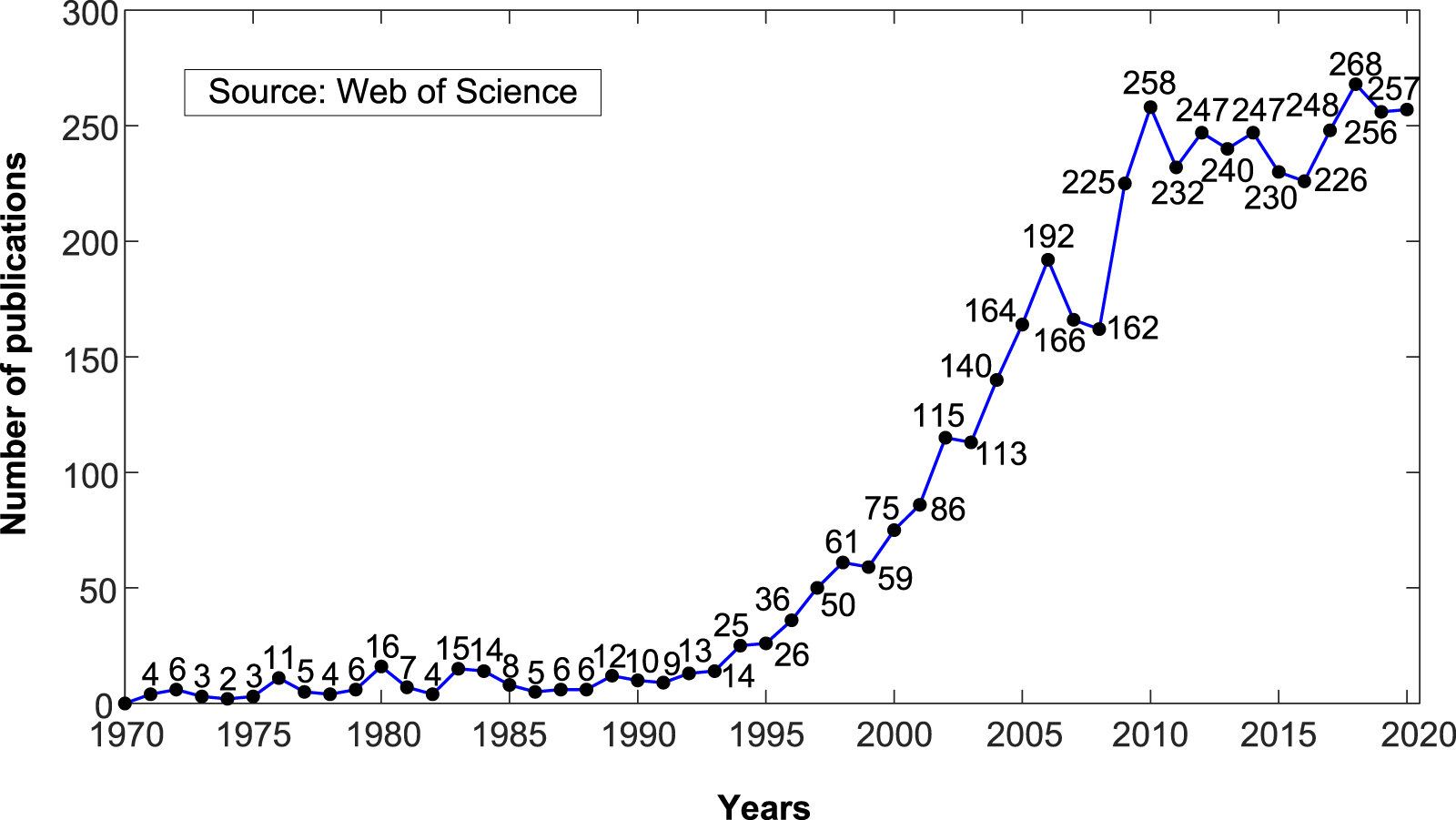
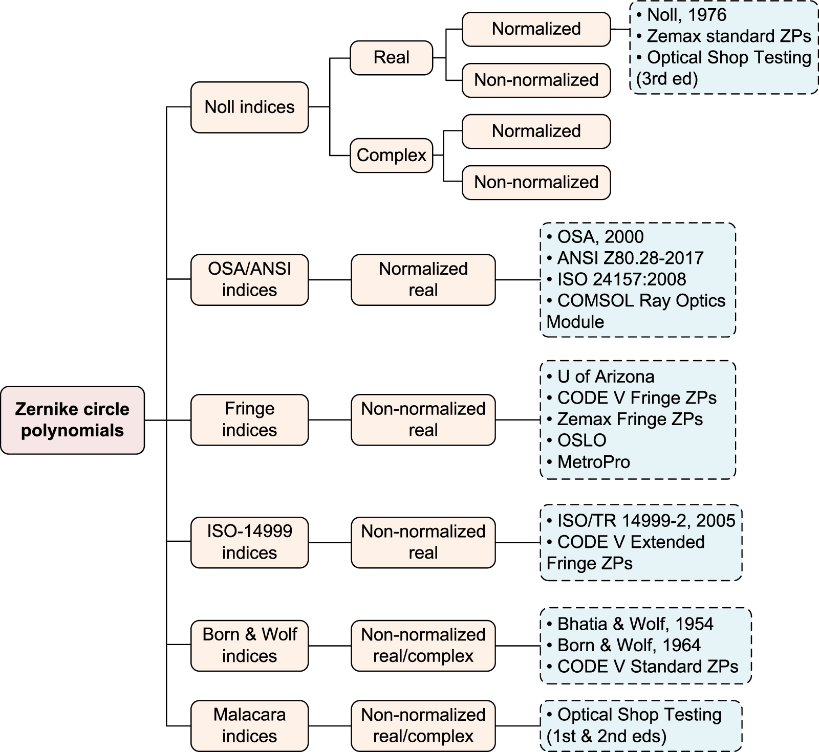
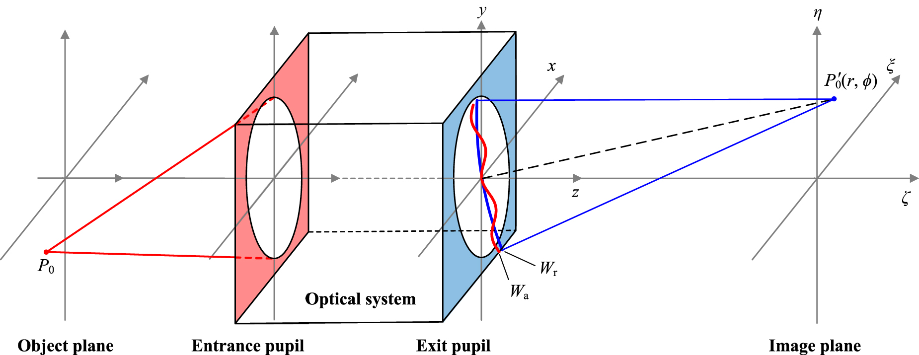
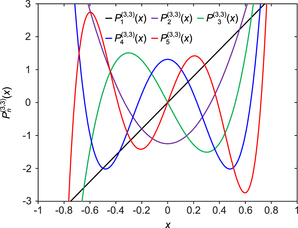
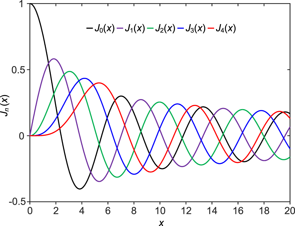
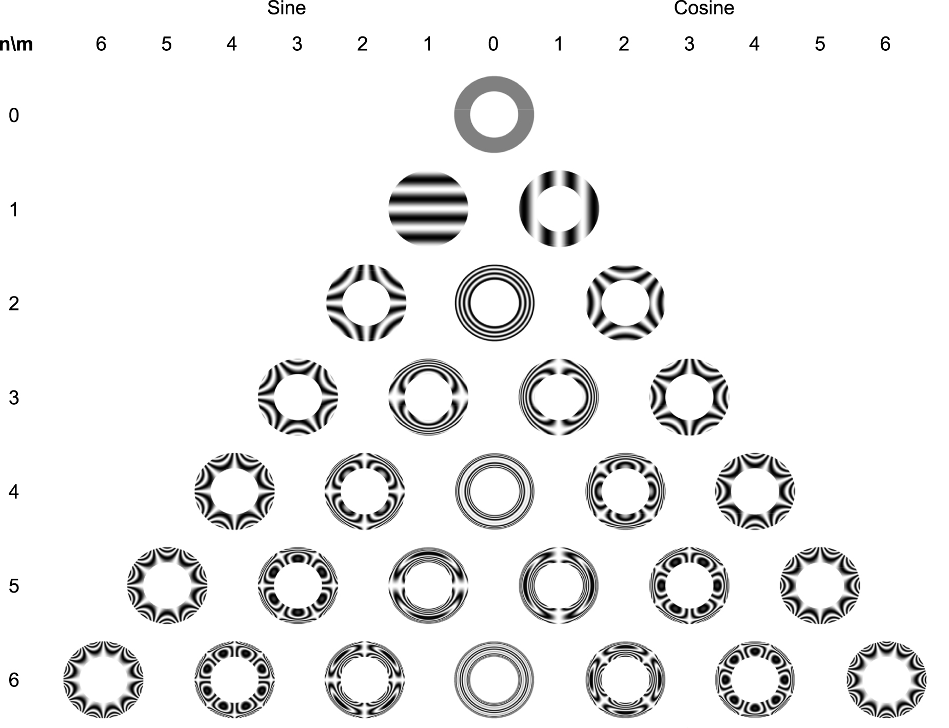
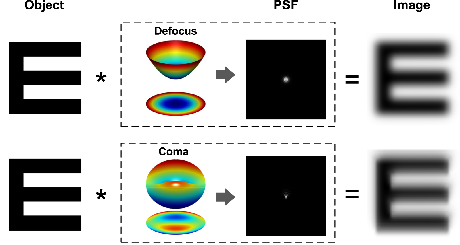
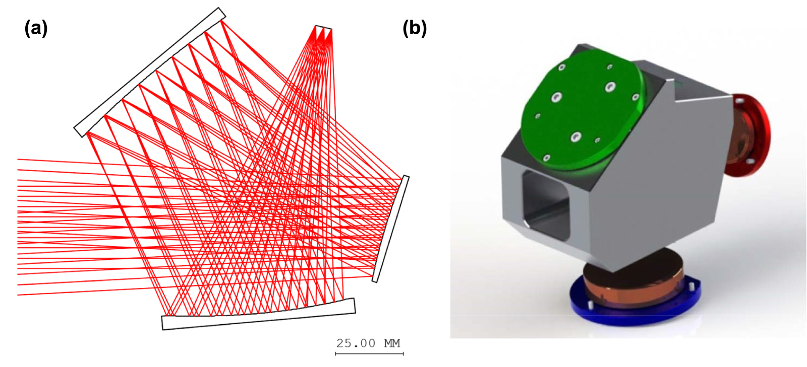
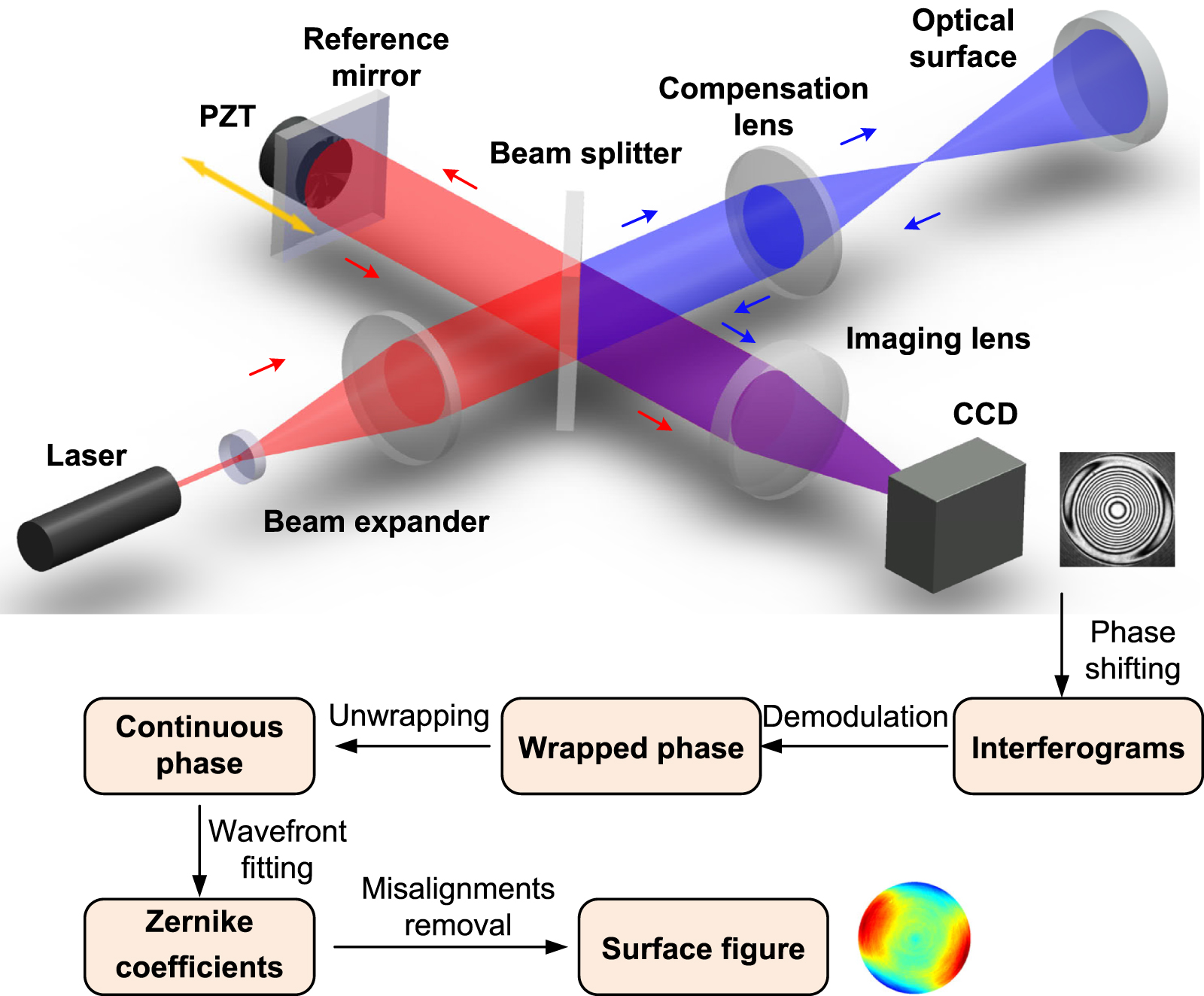
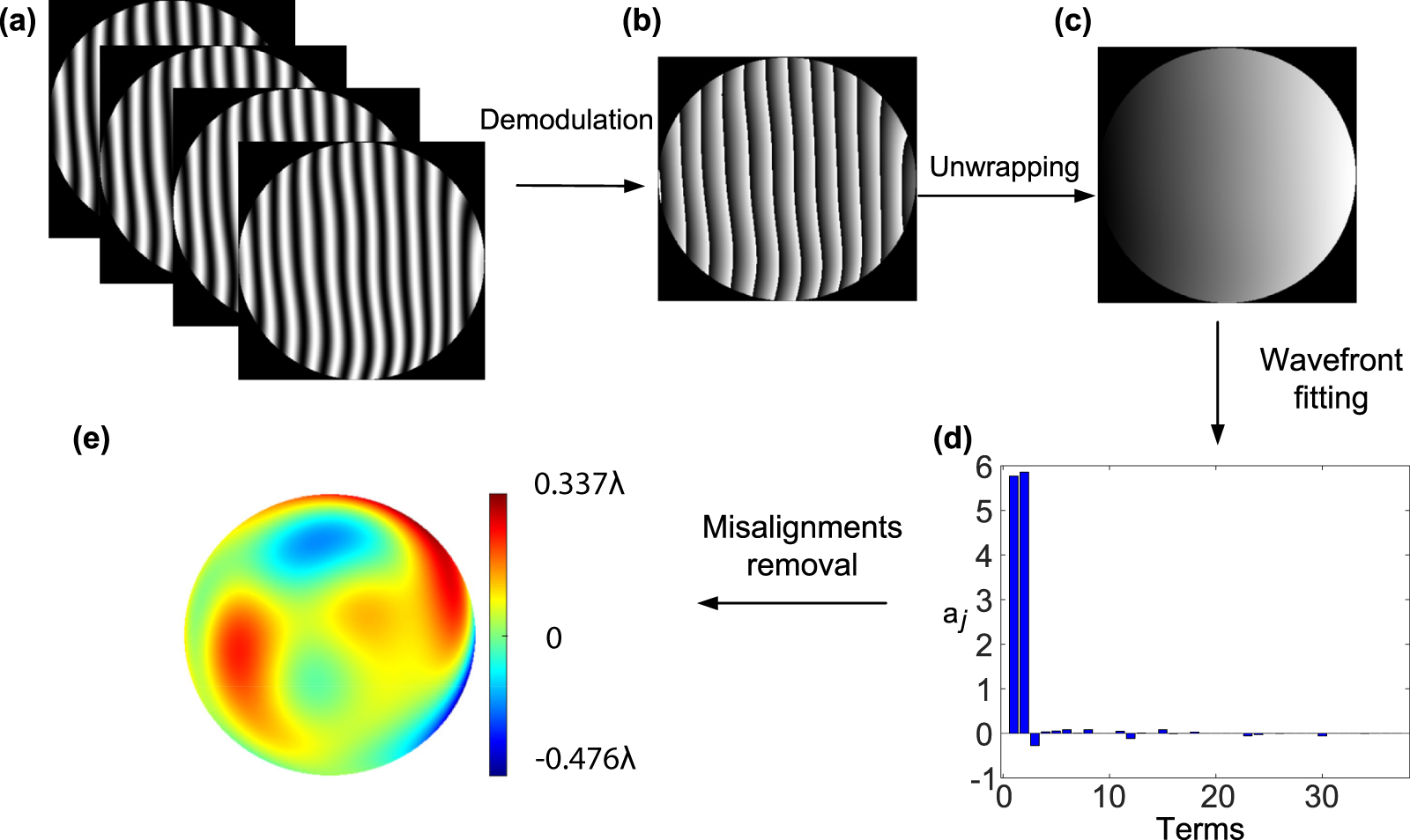
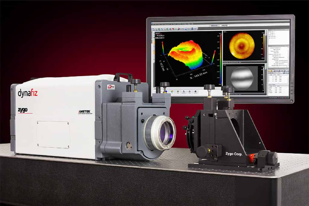
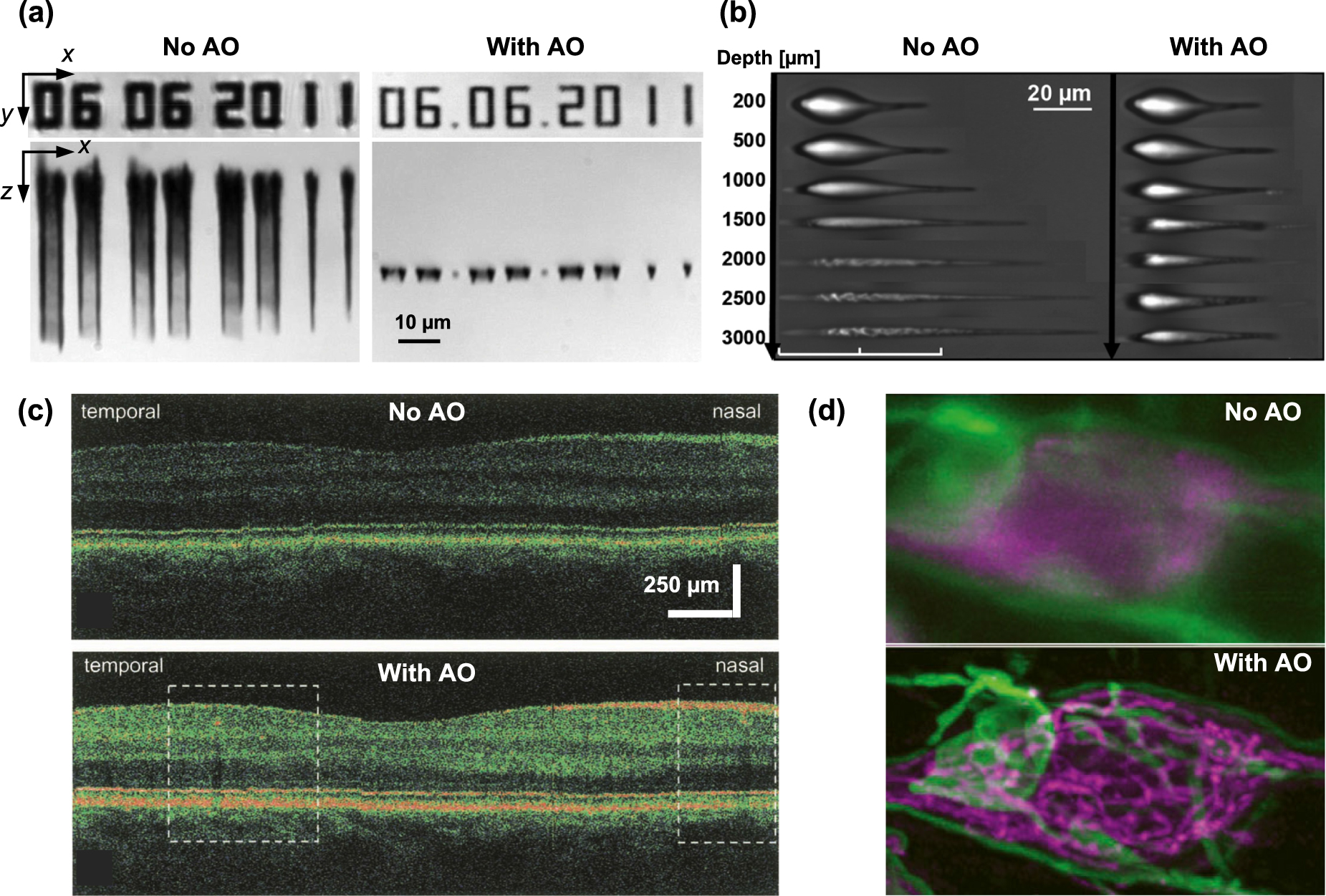
Figure 43. Zernike moments are rotationally invariant. From left to right: image rotated counterclockwise by an angle of 60 degrees.
Download figure:
Standard image High-resolution image
Table 19. Magnitudes of some Zernike moments for the rotated images in figure 43 and their statistics.

|

|

|

|

|

| |
|---|---|---|---|---|---|---|
| 0° | 29 686.85 | 2295.99 | 4959.74 | 3543.28 | 3219.67 | 1585.55 |
| 60° | 29 682.93 | 2296.33 | 4969.33 | 3543.65 | 3217.36 | 1584.38 |
| 120° | 29 685.44 | 2296.22 | 4964.34 | 3548.26 | 3220.37 | 1586.41 |
| 180° | 29 686.85 | 2295.99 | 4959.74 | 3543.28 | 3219.67 | 1585.55 |
| 240° | 29 682.93 | 2296.33 | 4969.33 | 3543.65 | 3217.36 | 1584.38 |
| 300° | 29 685.44 | 2296.22 | 4964.34 | 3548.26 | 3220.37 | 1586.41 |
| μ | 29 685.07 | 2296.18 | 4964.47 | 3545.06 | 3219.13 | 1585.47 |
| σ | 1.78 | 0.15 | 4.29 | 2.48 | 1.41 | 0.91 |
| σ/μ% | 0.006 | 0.007 | 0.09 | 0.07 | 0.04 | 0.06 |
Fast computation of Zernike moments is an important topic in Zernike moments based image analysis. To compute Zernike moments at lower degrees, one can directly use the explicit definition of Zernike polynomials. However, for Zernike moments at higher degrees, this method is not recommended because it involves the calculation of factorial functions present in the radial polynomial, which is computationally expensive [59]. In these cases, one can employ fast computation algorithms, such as the recursive methods based on the recurrence relationships of the radial polynomials (section 2.2.6) [59, 62, 64], among others [63, 188]. The recursive algorithms are reportedly more efficient and particularly suitable for fast calculation of Zernike moments.
As an important orthogonal moment, Zernike moments employ Zernike polynomials as the basis function and overcome the drawbacks of geometric moments. They have minimum information redundancy and can represent features in a more efficient, irredundant way. To date, Zernike moments have been widely used in many applications, such as pattern recognition [184, 189–191], multimedia watermarking [192, 193], and medical image analysis [194, 195].
4.6.2. Pseudo Zernike moments.
Pseudo Zernike moments stem from the pseudo Zernike polynomials (described in section 2.5.5), which are also a set of polynomials orthogonal over a unit circle analogous to the conventional Zernike polynomials. Pseudo Zernike moments, denoted by  , are defined as [48, 186]:
where  is the pseudo Zernike polynomials defined in equation (86), n is a nonnegative integer, l is an integer, and n − |l| ⩾ 0. Pseudo Zernike moments are analogous to conventional Zernike moments (equation (154)) and also hold the property of rotation invariance. However, they eliminate the constrain of n − |l| = even and thus have more moment invariants for the same degree n [Pseudo Zernike moments contain (n+ 1)2 invariants while Zernike moments have (n + 1)(n + 2)/2]. It is shown that pseudo Zernike moments are less sensitive to image noise than conventional Zernike moments [48]. Pseudo Zernike moments also have fast computation algorithms [196, 197] and have been used in a range of image analysis and pattern recognition applications [198, 199].
5. Discussion and conclusion
Although Zernike polynomials have been successfully used in a range of fields, it is important to be aware of potential pitfalls. First, Zernike circle polynomials are only orthogonal over a unit circle. For systems with non-circular pupils, such as annular and hexagonal pupils, Zernike circle polynomials are neither orthogonal nor represent balanced aberrations. In these cases, orthonormal polynomials can be constructed by orthogonalizing Zernike circle polynomials across the pupil [37, 105], as discussed in section 3.1. Second, Zernike polynomials are only orthogonal in a continuous fashion. This suggests that in general, they are not or at least not strictly orthogonal over a discrete set of data points in numerical simulation or real experiments. Potential errors should be taken into consideration when data points are sparse or unevenly distributed [200, 201]. Third, when comparing Zernike expansion coefficients of two wavefronts, it is important to specify the pupil diameters since the expansion coefficients vary with aperture size. This is especially true when comparing the aberrations of the eye from two measurements. Furthermore, Zernike polynomials may fail to represent some complex, irregular surfaces or shapes using a reasonable number of terms. Representative examples include fabrication errors present in the single-point diamond turning process [19] and irregular corneal aberrations of postsurgical or pathological eyes [202, 203].
In conclusion, we provide a comprehensive account of the development of Zernike polynomials in the past several decades, including the history, definitions, mathematical properties, roles in wavefront fitting, relationships with associated physical concepts, and connections with other polynomials, and survey their state-of-the-art applications. Potential pitfalls when using the Zernike polynomials are also discussed.
For Zernike polynomials over circular pupils, there are at least six different indexing schemes used by national and international standards, commercial software, and prominent scientists, including the Noll, OSA/ANSI, Fringe (University of Arizona), ISO-14999, Born and Wolf, Malacara indices. All indices share the same expression for the radial polynomials, which is the eigenfunctions of a second-order rotationally invariant partial differential equation [1, 6]. However, they differ from each other in naming, normalization, and indexing strategies, which are compared and summarized (table 8). Zernike polynomials possess rigorous mathematical properties, such as orthogonality and symmetry, and are closely related to other functions, such as XY monomials, Jacobi polynomials, Legendre polynomials, Bessel functions, and pseudo Zernike polynomials. Their Fourier transform, integration representation, derivative, and recurrence relations can be explicitly obtained to facilitate solving complex problems. Zernike polynomials are well-suited for wavefront analysis in optics because they have good corresponding relationships with Seidel aberrations. The wavefront fitting problem can be solved using the least-squares method. Expansion coefficients represent the standard deviations of corresponding aberration terms (except the piston term) and contain a wealth of information about the wavefront. The expansion coefficients can be easily transformed when the original wavefront is translated, rotated, or resized (section 2.3.2).
Zernike circle polynomials are only orthogonal over the interior of a unit circle. Polynomials orthogonal over non-circular pupils can be constructed based on Zernike circle polynomials. The most commonly used construction approach is the recursive Gram–Schmidt orthogonalization method. Based on this method, orthonormal polynomials over five noncircular pupils, including annular, rectangular, square, hexagonal, and elliptical pupils common in optics, are discussed. The orthonormal polynomials over annular pupils, called Zernike annular polynomials, are reviewed with emphasis due to their practical significance. The Zernike annular polynomials are defined based on the Noll indices and their recurrence relations and Fourier transform are explicitly presented. The Zernike annular polynomials have similar corresponding relationships with Seidel aberrations as Zernike circle polynomials and are well-suited for wavefront analysis over annular pupils.
In addition, we also survey state-of-the-art applications of Zernike polynomials in a range of fields, including the diffraction theory of aberrations, optical design, optical testing, ophthalmic optics, adaptive optics, and image analysis. In the diffraction theory of aberrations, Zernike polynomials are used to expand the wavefront aberration at the exit pupil of an optical system and corresponding expansion coefficients are used to compute the PSF at the image plane according to the (extended) Nijboer–Zernike theory. In optical design, Zernike polynomials are used to analyze the wavefront aberration of a designed optical system, represent freeform surfaces, and facilitate system optimization. In optical testing, Zernike polynomials are used to fit measured interferometric wavefronts and remove misalignment errors. In ophthalmic optics, Zernike polynomials are used to reconstruct ocular wavefront measured by a Shack–Hartmann wavefront slope sensor and report optical aberrations of the eye. In adaptive optics, Zernike polynomials are used for the representation, reconstruction, and compensation of optical wavefronts distorted by atmospheric turbulence. In image analysis, Zernike polynomials are used to define Zernike moments and pseudo Zernike moments, which hold the property of rotation invariance and can be used as shape descriptors for pattern recognition.
This review is aimed to clear up the confusion of different indexing schemes, provide a self-contained reference guide for beginners as well as specialists, and facilitate further developments and applications of Zernike polynomials.
Acknowledgments
We thank Xiaoxiao Ma, Heren Li and Jin Wei for proofreading the manuscript. This work is supported in part by the National Natural Science Foundation of China (NSFC) under Grant Nos. 62122072, 12174368, and 61705216, the National Key R&D Program under Grant No. 2022YFA1404400, the Institute of Artificial Intelligence at Hefei Comprehensive National Science Center under Grant No. 21KT016, the Anhui Science and Technology Department under Grant Nos. 202203a07020020 and 18030801138, the Zhejiang Lab under Grant No. 2019MC0AB01, the Research Fund of the Chinese Academy of Sciences (CAS), and the Research Fund of the Double First Class Initiative.
Data availability statement
The data generated and/or analyzed during the current study are not publicly available for legal/ethical reasons but are available from the corresponding author on reasonable request.
Conflict of interest
The authors declare no conflicts of interest.