

Abstract
We consider the general problem of matching rheological models to experiments. We introduce the concept of identifiability of models from a given set of experiments. To illustrate this in detail, we study two rheology models, the grade-two and Oldroyd 3-parameter models, and consider two hypothetical rheometers to see if the coefficients of the rheology models are identifiable from experimental measurements or not. For the Oldroyd models, we show that the coefficients can be estimated from experiments from the two rheometers. But for the grade-two model, it is not possible to distinguish the two nonNewtonian parameters, only their sum can be estimated, and thus the grade-two model is not identifiable by the two hypothetical rheometers. However, our results imply that a different rheometer may be able to do that.
Export citation and abstract BibTeX RIS

Content from this work may be used under the terms of the Creative Commons Attribution 4.0 licence. Any further distribution of this work must maintain attribution to the author(s) and the title of the work, journal citation and DOI.
Recommended by Professor Hyung Jin Sung
There are many models for non-Newtonian fluids, as highlighted by the so-called Rheology Drugstore of Joseph (2013). Similarly, there are many types of rheometers (Lodge et al 1991, Gallot et al 2013, Nyström et al 2017) designed to measure the properties of different fluids. Our goal here is to consider a small subset of each and ask the question: to what extent do the rheometers distinguish coefficients in different models?
The next objective is to turn this question around, and ask what coefficients in different models best match experimental data, and ultimately, which model bests fits the experiments (Robert et al 1985). However, the prerequisite for such a study is the requirement that given rheometers can distinguish the different parameters, a property that we can describe as identifiability.
To begin this study, we consider two different rheology models: the grade-two model (Girault and Scott 2001) and the Oldroyd models (Girault and Scott 2018). We chose these models in part because of the Tanner (1982), Girault and Scott (2021a, 2021b)duality property for these models. There are of course many other models that are used for rheology. One simple but popular one is the power-law model. This has been extensively studied (Saramito 2016).
We begin by considering geometries and flow profiles that provide exact solutions for these models, for two reasons. First of all, they give test problems for computer simulation codes. But more importantly, they allow a clear view of what a given rheometer will distinguish in a given model, or not. More realistic rheometer designs are considered in Pollock and Scott (2022b).
We describe two hypothetical rheometers related to the exact solutions for the two models, both of which involve two parameters in addition to viscosity. We will show that the Oldroyd model is identifiable with these two rheometers but the grade-two model is not. On the other hand, recent computational evidence (Pollock and Scott 2022b) indicates that the grade-two model is identifiable by a contraction rheometer (Nyström et al 2017).
The state of rheology model theory has advanced recently with the advent of rigorous mathematical analyses of some models (Cioranescu et al 2016). This includes both the establishment of a foundational theory for the system of partial differential equations and associated boundary conditions, as well as numerical methods for solving the equations. Despite recent advances in these directions (Pollock and Scott 2022a, 2022c), much still needs to be done to clarify important properties of popular models. A review of Bird et al (1987) indicates the breadth of models that would need to be considered.
We limit our purview to steady flows. Determining rheological properties from time-dependent flows is likely much more complicated.
1. Rheology modeling challenge
The challenge of rheology modeling is to match apples and oranges. Let us say that the apples are the models, of which there are many (Joseph 2013), and they have many parameters. The oranges are rheological measurements, done by devices called rheometers, essentially machines that do experiments to determine quantities such as a force as a function of flow rate.
Experimental quantities and concepts include
- normal-stress difference (Lodge et al 1991),
- excess pressure drop (Nyström et al 2017)
- extensional viscosity (Petrie 2006),
- apparent viscosity (Tanveer et al 2006),
- shear thinning/thickening (dilatant),
- rheopectic versus thixotropic (time dependent).
How do we match them to models? A quote by Pearson in Petrie (2006) sums up the challenge this way:
'... if you want to predict flow in all circumstances, you need a REoS [a rheological equation of state or constitutive equation], nothing less. Rheometric functions can be useful in classification and categorization, involving qualitative statements, and can provide engineering approximations in particular flow fields, but they cannot be inserted in CFD packages.'
In a very simple case, we can consider a particular model (e.g. Oldroyd) and ask how we can determine its parameters x from the measurements y of a given rheometer, or multiple rheometers. What computational simulations of rheometers produce is  . But we want to determine an inverse function
  . To do so, we need to know if the given rheometer can distinguish the parameters x of the model. That is, for different values of x, do you get some different data y? If not, then there could be multiple x for a single y, and so g is not a function. We will see that, for example, measurements from a shear-flow rheometer will be identical, independent of the key parameter of the grade-two model. Thus it may not be possible to find a function g just using that one rheometer.
The parameters of a model cannot be reliably determined from a single experiment, or even a number of experiments matching the number of parameters. Rather, a larger set of experiments are used to determine parameters. For example, this can be done by varying the flow rate, and thus the Reynolds number, e.g. by simply increasing the flow rate as a function of time and measuring the resulting experimentally determined data. The flow rate can be stabilized at different times to insure steady flow is established at each successive Reynolds number.
2. Rheology models
All models of steady flow have the basic equation

where T is the extra (or deviatoric) stress. The models only differ depending on how the stress is related to the velocity u. In the case of a Newtonian fluid

where ν is the kinematic viscosity (Landau and Lifshitz 1959) and  . Thus, when
  , it follows that
  , and we obtain the well known Navier–Stokes equations for Newtonian flow,

where f is a possible body force. Table 1 gives the kinematic viscosity ν for various fluids at various temperatures. One feature indicated by the table is that gases increase in viscosity as temperature is increased, whereas liquids decrease in viscosity as temperature is increased. The unit chosen (stokes) makes it natural to measure lengths in centimeters and fluid speeds in centimeters per second. For many rheometers, these are natural units.
Table 1. Kinematic viscosity coefficients in stokes (cm2 s−1) for various fluids (Kestin et al 1978, Gokdogan et al 2015).
| Fluid | Kinematic viscosity | Conditions |
|---|---|---|
| Castor oil | 2.41 |
 40 40  104 F 104 F |
| Air | 0.100 |

 F F |
| Air | 0.170 |
 40 40  104 F 104 F |
| Water | 0.010 |
 20 20  68 F 68 F |
| Water | 0.006 |
 45 45  113 F 113 F |
| Mercury | 0.001 |
 20 20  68 F 68 F |
Typically, nonhomogeneous boundary conditions are imposed:  on
on  , the bounding surface of the volume Ω.
2.1. Viscosity definition
The dynamic (or absolute) viscosity µ is defined typically as the ratio of stress σ and strain rate:

Stress is defined as the force per unit area across an infinitesimal surface. Force has units  , so stress has units
  . Therefore the units in (2.3) are consistent. But v and x are vector quantities, so in general µ would have to be a tensor of order (or arity) 4 in general (Nunan and Keller 1984). For Newtonian fluids, this tensor reduces to a scalar times the identity tensor.
The units of µ are mass divided by length×time, and the units of mass density ρ are mass divided by length cubed. Thus the units of  are
are

which are the units for diffusion.
The kinematic viscosity ν is simply  . Table 1 gives the kinematic viscosity for various fluids under various conditions.
2.2. Apparent viscosity
Apparent viscosity is typically defined as (2.3) without significant elaboration. In Nijenhuis et al (2007), more complicated notions are explored. But there are various ways to generate v and the resulting σ will often have several components. So a precise experimental or computational framework is necessary to make a clear definition. Here we will give two such examples. We will see that the ultimate relationship is tensorial, so it is not so clear how to define a scalar value for 'viscosity.' Indeed, we seem to be lacking a good term to explain the principal effect of rheology beyond Newtonian viscosity. One way is simply to define the apparent viscosity νa as

for some norm on matrices, where T is the observed stress related to the flow velocity v. The same fluid could produce different values of apparent viscosity in different flow geometries, however.
2.3. Thin/thick-ening
If we use the definition (2.4) for apparent viscosity, then we can say that the fluid is thinning if

when t > 1. When this holds for the expression (2.4) involving a norm, then any other notion thinning would also apply. But (2.4) may be too strong to catch subtle behaviors.
Thickening would involve the reverse inequality:

when t > 1. Often, the terminology suggests a particular flow regime such as shear, which we will study. But we will also consider a flow problem involving pure extension, in which  has quite different structure.
3. Oldroyd models
The simplest subset of the Oldroyd models involves three parameters, the fluid kinematic viscosity ν and two rheological parameters λ1 and µ1. This subset lacks any explicit dissipation mechanism, and Renardy (1985) suggested one way to incorporate one. Another approach was explored in Girault and Scott (2018) that has a strong theoretical base and provides an algorithm for approximation.
A three parameter subset of the eight parameter model of Oldroyd (1958) for the extra stress takes the form

where the five parameters λ2, µ2, µ0, ν0, and ν1 in Oldroyd (1958) are set to zero, and

We have used the notation  to mean tensor multiplication, which is in this case the same as matrix multiplication. Note that
  ,
,  ,
,  , and
, and  .
.
We can write the full model in the steady case as


The general case (3.6) can thus be written similarly as

When  , (3.6) is known as the upper-convected Maxwellian model (Tanner 1982, Renardy 1985):

When  , (3.6) is known as the lower-convected Maxwellian model. There are physical reasons to assume that
  , but we will allow
  as well. The case
  corresponds to the incompressible Navier–Stokes equations.
The difficulty with this set of Oldroyd-type models is that there is no explicit dissipation (Girault and Scott 2018) in the basic equation (2.1).
3.1. Extensional flow
For a given constant speed U, extensional flow  , depicted in figure 1, exhibits a constraint for the Oldroyd models. This flow is evidently incompressible, and we will show that there is a corresponding solution with constant T, so that
  . We have

Thus
so we can take

and solve

for any β.

Figure 1. Extensional flow in a two-dimensional channel.
Download figure:
Standard image High-resolution image3.2. Extensional stress for 3 parameter Oldroyd
If we take
then (3.6) (for constant T) simplifies to

Suppose that

for unknown constants a, b, c. Then

From (3.8) and (3.11), we conclude that
Thus b = 0 and

We can simplify this using the expressions

with  . Thus there is a solution with constant T given by
for extensional flow  . The first part of the stress T is the Newtonian stress
and the second part we can think of as the Oldroydian part:
There is a well known singularity (Owens and Phillips 2002) for flow at speed

For  , the coefficient a becomes singular for this value of U, and if µ1 were negative, the coefficient c in (3.12) would be the one to indicate a singularity, instead of a. The limitation U on µ1 can be viewed as a defect, but it can also be viewed as just a feature of the model. That is, it says that there is a limit on the size of
  related to the range of appropriate flow speeds being modeled.
By considering extensional flow for the Oldroyd model, we have learned that
- the parameter µ1 can be very small and yet have a big effect, and
- the Oldroyd stress in extension does not depend directly on λ1.
3.3. Extensional rheometer
We can imagine an extensional rheometer where we measure the normal stress on the outlet of the channel

where  and L indicates the end of the channel. Physically, we could put a membrane over the outlet and measure its deformation, at least for small deformations. The integral of the normal stress gives the force on the membrane.
If we are mainly interested in how (3.16) differs from Newtonian flow, this simplifies to be

since the pressure is the same for Newtonian flow. Thus the Oldroyd fluid can be shear-thickening or shear-thinning depending on the sign of µ1.
3.4. Computing coefficients from data
The force F measured in the extensional flow rheometer, that is the Newtonian component together with the non-Newtonian force in (3.17), is

where (3.9) implies that

We claim that plotting (3.18) as a function of U allows identification of ν and µ1, although it would give no information on λ1. We will demonstrate this as follows.
We can measure the slope  from the plot of (3.18) as a function of U to get

We have  . In particular, this shows that the extensional rheometer can measure the viscosity. Moreover,
where

Differentiating (3.21) with respect to U, we find

Thus

so that  . Therefore
But
Thus

Moreover,

so g is monotonically increasing. From (3.26)

Since g is monotonically increasing, the function φ defined by

is also monotonically increasing for  . Thus we can write

Note that solving  can easily be done via Newton's method. Both the slope and its derivative can be obtained reliably from the data via the Savitsky–Golay algorithm (Scott and Scott 1989). The value of µ1 can thus be reliably estimated by averaging (3.29) over a suitable range of U values. A plot of
  is in figure 2.
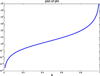
Figure 2. Plot of  where g is defined in (3.25).
Download figure:
Standard image High-resolution imageTo get a more precise understanding of the behavior of µ1 on the data, we can also write

Then
Therefore, q is strictly increasing for  . For U small, we have

so that
and hence

We do not need to differentiate the slope of the data twice to compute µ1 via the formula (3.29). Inverting the function φ can be done numerically to high accuracy via Newton's method, without relying on any smoothness of the data.
3.5. Shear flow
We consider two-dimensional flow in a channel ![${\Omega} = [-L,L]\times [0,1]$](https://content.cld.iop.org/journals/1873-7005/55/1/015501/revision3/fdracafa1ieqn50.gif) . Couette, or shear, flow, has
. Couette, or shear, flow, has  and p constant if T is constant as shown in figure 3. Now we consider (3.7). We have
and suppose that

Then

Similarly,

Therefore
Therefore the equation
reduces to

so that

Therefore
Thus

and so

Let us define the stress  for Newtonian shear flow by

and we can denote the Oldroyd stress (3.36) by  . Then


Figure 3. Shear flow in a two-dimensional channel. the upper channel wall is moving.
Download figure:
Standard image High-resolution image
3.6. Shear rheometer
We can imagine a rheometer based on shear flow, as follows. We have a rotating belt at the top of the channel enforcing the velocity  . If we did not constrain the bottom of the channel, the whole apparatus would move to the right. So we measure the force required to keep it in place. This force must be balanced by the fluid shear stress

Here,  is the outward normal to the bottom of the channel, and
  is tangent to the bottom. But

so that

Thus the force measured for an Oldroyd fluid is the same as that measured for a Newtonian fluid, multiplied by
Plotting
as a function of U would allow identification of both ν and  , but it would not determine λ1 and µ1 separately. But if we combine this with the results of the extensional rheometer, we can recover λ1, although the sign would be ambiguous. In particular,

Thus
Note that for small U,

so that
remains bounded as U → 0.
3.7. Oldroyd rheometer conclusions
We have shown that a shear-flow rheometer can be used to determine both ν and the combination  , whereas the extensional-flow rheometer can be used to determine both ν and µ1, but not λ1. Combining measurements from these two rheometers allows the determination of all three coefficients, and it includes a cross check on the viscosity parameter ν.
4. Grade-two fluid model
The grade-two model of Ericksen and Rivlin (1997), Girault and Scott (1999) can be expressed as a single equation. The stress tensor for the grade-two fluid model satisfies
where  and the material derivative and the lower-convected Oldroydian derivative are given by

for any tensor-valued function f. For the steady-state, grade-two fluid model, the stress tensor simplifies to

where the operator  is just matrix multiplication, but it has been made explicit to simplify interpretation. Thus the equations of steady fluid motion (2.1) can be written

Here

4.1. Extensional flow
We saw in section 3.2 that extensional flow, given by
is a solution of the Navier–Stokes equations (3.10) in the domain depicted in figure 1. Thus we also have a solution of the grade-two model in that domain provided that

is constant. Since  is symmetric in this case, we have
and thus  and
and

where  is the identity matrix. Thus the expression in (4.47) is constant. Then
4.2. Extensional flow rheometer
The extensional flow rheometer would report a difference from Newtonian flow for the normal stress at the outlet given by
Thus the grade-two fluid can be shear-thickening or shear-thinning depending on the sign of  .
.
The force measured will be a combination of ν and  , namely
where cp
is defined in (3.19). By plotting the measured force against U, it is possible to determine both ν and  .
.
4.3. Shear flow: grade two
We saw in section 3.5 that  and p is constant if T is constant. We have
Thus (4.44) implies that

Here we have  where
where

4.4. Shear flow rheometer
The shear-flow rheometer described in section 3.6 for the grade-two model will measure the same quantity as in (3.39) but with  replaced by
  . And like the Oldroyd model,
  , so the simple shear rheometer will give the same result as for a Newtonian fluid, independent of the parameters αi
. Thus a pure shear-flow rheometer will report ν and a pure extensional flow rheometer will report a combination of ν and
, so the simple shear rheometer will give the same result as for a Newtonian fluid, independent of the parameters αi
. Thus a pure shear-flow rheometer will report ν and a pure extensional flow rheometer will report a combination of ν and  . Combining the two rheometers, we can determine
  , but it does not seem possible to determine α1 and α2 separately with these two geometries alone.
4.5. Grade-two rheometer conclusions
We have seen that the simple shear-flow rheometer described here does not distinguish the coefficients α1 and α2 in the grade-two model, despite the fact that the induced stress difference  is quite complex in shear. If we take the definition (2.4) for apparent shear, then the grade-two model is shear thinning when α2 is sufficiently negative, and otherwise it is shear thickening (assuming
  in both cases).
5. Tanner duality
Tanner (1982) realized that there is a duality between the grade-two model (Girault and Scott 2001) and the Oldroyd models Girault and Scott (2018). This duality has been studied more recently from a mathematical perspective (Girault and Scott 2021a, 2021b). More precisely, Tanner observed that the solutions of grade-two were asymptotically the same as those for Oldroyd, with the parameters related by

For clarity, let us write  for the total Oldroyd stress, and
  for the total grade-two stress. We also write
  for the Newtonian stress. With the parameters related by (5.50), we expect that as
  ,
,

for fixed flow rate U and viscosity ν. Since we have computed stresses for these models in shear and extensional flow, we can compare them to test the range of validity of Tanner duality.
5.1. Extensional stresses
For extensional flow (section 3.1), the Newtonian stress  and Oldroyd stress
  are given in (3.14):

Thus  . By contrast, the grade-two stress
  is given in (4.48) as

where we have invoked (5.50). Thus we see that  . But more importantly, we can use (3.13) to show that
in agreement with Tanner duality. On the other hand,  and
and  diverge rapidly as
  in accordance with (3.15). Note that
  displays no singularity in this limit.
5.2. Shear stresses
For shear flow (section 3.5), the Newtonian stress  and Oldroyd stress TO
are given in (3.38):
and Oldroyd stress TO
are given in (3.38):
Therefore

By contrast, the grade-two stress  is given in (4.49) as
Therefore invoking (5.50), we see that

Thus

again confirming Tanner duality.
5.3. Model complementarity
Tanner duality allows us to pick models appropriately that match certain experiments. Let us re-examine shear flow and postulate a rheometer that measures the normal force on the top and bottom of the domain. Such a theoretical rheometer shares some features with the Lodge rheometer (Lodge et al 1991).
Let us simplify to the case where  . The Newtonian stress contributes nothing to the normal force, and the pressure is constant in shear flow, so the normal force is proportional to λ1 for the Oldroyd model and
  for the grade-two model, where the constants of proportionality have the same sign. We can imagine two complementary materials A and B, one that pushes out on the channel walls and one that pulls in, as the fluids are sheared. Both types of materials are known in solid mechanics, so one cannot say a priori either is unrealistic. Then picking the Oldroyd model for material A might require
  , which has several drawbacks from a modeling perspective. Correspondingly, picking the grade-two model for material B would require
  , with its own set of drawbacks. However, picking the Oldroyd model for material B would have
  due to Tanner duality, so it would be the preferred model for simulation. Similarly, picking the grade-two model for material A would have
  due to Tanner duality, so it would be the preferred model for simulation.
6. Real rheometers
There is a variety of actual rheometers that are employed to make measurements. Here we describe just a few.
6.1. Contraction rheometers
A rheometer that emphasizes extensional flow is based on a contraction nozzle (Nyström et al 2017). Fluid is forced through the contraction either by pressure or a rod. The flow domain is defined by

for a given function f.
Since the two theoretical rheometers fail to detect α1 for the grade-two fluid, a natural question is whether or not a contraction rheometer can do so. Since the extensional flow rheometer detects  , a natural approach is the consider the special case
  , for which the grade-two model simplifies (Girault and Scott 1999, 2001). Similarly, it makes sense to consider a two-dimensional contraction as a first step, again simplifying the grade-two model. Such a geometry is considered in Pollock and Scott (2022b).
6.2. Counter-rotating cylinders
One common type of rheometer is based on counter-rotating concentric cylinders, essentially the original experiment of Couette (Gallot et al 2013). What is measured is the torque on one cylinder induced by the other cylinder. For example, the outer cylinder is rotated at a fixed speed and the torque on the inner cylinder required to keep it stationary is recorded. This measures quantities similar to our pure shear rheometer, so we do not pursue this further here.
6.3. X-plate rheometers
There are two different, but related rheometers that involve a plate below and either (a) a cone above or (b) a parallel plate above. For example, the lower plate could be fixed and the upper structure rotated. Thus one obtains the cone-and-plate rheometer (Markovitz et al 1955, Ellenberger and Fortuin 1985) and the parallel-plate rheometer (Yamamoto 1958, Ellenberger and Fortuin 1985). In both cases, the geometry and (steady) flow have radial symmetry.
6.4. Hole-pressure difference rheometer
Lodge (1996) constructed a device to measure normal stress differences. The flow in a two-dimensional version of this device has been proposed as a test problem (Lodge et al 1991). Such approaches have been used effectively in rheological measurements in food technology (Padmanabhan and Bhattacharya 1993).
6.5. Journal bearing flow
In Robert et al (1985), two-dimensional computational simulations of journal bearings were used to evaluate six different rheological models.
7. Thick or thin
We summarize here the results of the exact solutions for both rheological models. Our objective is help assess whether models are thinning or thickening in different contexts. There are two issues to consider. First of all, does the stress change with changing flow rate or strain rate in a substantial way? If it does, does a particular rheometer report that change? We have noted the shortcoming of the shear rheometer for grade-two fluids. But we can see that it is not due to a lack of change of the stress itself.
Since the stress is a symmetric tensor, in two dimensions any stress can be written in terms of three basis vectors:

In general, we can write

Suppose we choose the norm in (2.4) to be the Frobenius norm
This is the norm associated with the inner-product
In this inner-product,  ,
,  , and
, and  are all orthogonal and have Frobenius norm equal to
  . Thus

Now let us use the representation (7.60) to describe our previous calculations of stresses in different flow regimes.
7.1. Oldroyd extensional flow
We first need to resolve the matrix on the right in (3.14). Using (7.60), we have
Therefore
Thus
The strain (3.8) for extensional flow is proportional to U, so the apparent viscosity (2.4) tends to infinity as  , and this would be described as extensional thickening.
7.2. Oldroyd shear flow
From (3.38), we find

If  , this simplifies to
In this special case,
and asymptotically as  ,
,
In the general case,
If  , then
as  . This would qualify as shear thinning, since (3.33) implies that the Frobenius norm of the strain is proportional to U.
7.3. Grade-two extensional flow
From (4.48), we find

Thus

Since the strain (3.8) for extensional flow is proportional to U, the apparent viscosity (2.4) grows monotonically as U increases, and this would be described as extensional thickening.
7.4. Grade-two shear flow
From (4.49), we find

Thus

Again, the strain (3.8) for shear flow is proportional to U, so the apparent viscosity (2.4) grows monotonically as U increases, and this would be described as shear thickening.
7.5. Other metrics
A norm is blunt instrument, but we saw in section 7.2 that it can identify shear thinning. But there may be a finer tool to analyze the impact of stress. The expression  is the force on the plane perpendicular to the unit vector n due to the stress
σ
. Then
is the force on the plane perpendicular to the unit vector n due to the stress
σ
. Then  is the force due to
σ
in the direction n, that is, against the surface represented by the plane. It t is another direction, then
is the force due to
σ
in the direction n, that is, against the surface represented by the plane. It t is another direction, then  is the force due to
σ
in the direction t. One direction of interest would be a direction tangent to the plane.
is the force due to
σ
in the direction t. One direction of interest would be a direction tangent to the plane.
In the two-dimensional case, we can use the decomposition (7.60) for stresses and take t to be orthogonal to n and consider the force magnitudes
These represent the 'observables' for
σ
. Note that for symmetric
σ
,  .
.
To quantify this, let us assume that

Then we have


Therefore

We recognize the matrix in (7.64) as a rotation by  .
.
As a first application, let us apply this methodology to Newtonian fluids. For shear flow,  , and for extensional flow,
  . Thus
For example, if we take θ = 0 (meaning the plane is perpendicular to the x-axis), then the normal force on this plane would be proportional to  in extensional flow (with the shear stress zero), whereas the tangential force on this plane would be proportional to
  in shear flow (with the normal stress zero).
As another application, we apply this methodology to grade-two shear flow. Then

For θ = 0, the normal force on the plane perpendicular to the x-axis is proportional to  . This could be measured with a net held initially in this plane, the deformation of the net being proportional to the force. Together with the measurement of
  via the extensional flow rheometer, α1 can then be determined.
8. Conclusions
We have studied the grade-two and Oldroyd 3-parameter models, and we computed solutions relevant to two hypothetical rheometers to see if the coefficients of the rheology models are identifiable from experimental measurements or not. For the Oldroyd models, we showed that the coefficients can be estimated from experiments from the two rheometers. But for the grade-two model, it was not possible to distinguish the two nonNewtonian parameters, only their sum can be estimated.
Acknowledgments
We would like to thank Sara Pollock and Tabea Tscherpel for valuable discussions. We also thank the referee for valuable suggestions.