
Abstract
Magnetic fluids have been around since the 1940s. They come in different forms: magnetorheological fluids (MR fluids) and ferrofluids. MR fluids characterise themselves by having a large change in viscosity under the influence of a magnetic field. Ferrofluids have a significantly smaller change in viscosity, however ferrofluids are colloidal suspensions. After their discovery many applications followed, such as the MR clutch, magnetic damper and bearing applications, in which the fluids are subjected to ultra high shear rates. Little information is available on what happens to the rheological properties under these conditions. In general, the characteristics determined at lower shear rates are extrapolated and used to design new devices. Magnetic fluids have potential in the high tech and high precision applications and their properties need to be known in particular at shear rates around 106 s−1. Commercially available magnetorheometers are not able to measure these fluids at ultra high shear rates and are limited to 105 s−1. Therefore a new magnetorheometer is required to measure ultra high shear rates. In this paper the physical limitations of current measuring principles are analysed and a concept is designed for ultra high shear rate rheometry in combination with a magnetic field. A prototype is fabricated and the techniques used are described. The prototype is tested and compared to a state of the art commercial rheometer. The test results of the prototype rheometer for magnetic fluids show its capability to measure fluids to a range of 104 s−1– s−1 and the capability to measure the magnetorheological effect of magnetic fluids.
Export citation and abstract BibTeX RIS

Original content from this work may be used under the terms of the Creative Commons Attribution 3.0 licence. Any further distribution of this work must maintain attribution to the author(s) and the title of the work, journal citation and DOI.
1. Introduction
Magnetic fluids come in different forms with different properties. Commonly they are known as magnetorheological fluids (MR fluids) and ferrofluids. In the 1940s Jacob Rabinow created the first MR fluid. These MR fluids alter their rheological properties (viscosity) significantly under the influence of a magnetic field. The first use of ferrofluids is credited to Papell while working for NASA in 1963 [1]. Ferrofluids have significantly less change in their viscosity, however, are the first magnetic fluids that are colloidal suspensions [2–4]. Due to their unique characteristics these magnetic fluids quickly found their applications. In 1948 Rabinow patented the first application of a MR fluid, the MR clutch [5]. Soon after he patented the MR force transmitter [6]. Later on came applications such as magneto rheological damper [7], MR brake [8] and many more [9, 10].
Ferrofluids found applications in bearing applications [11, 12], dynamic sealing applications [13] and more [14].
In these systems the fluid flows at high speed. For example fluid bearings typically have a thin film (10  m) and rotate at high speed (10 m s−1). Little knowledge is available about what happens to the fluid characteristics at these speeds. Prior research has reached shear rates up to 105 s−1 [15–18].
Commercial rheometers are not designed to measure at high shear rates (above 104 s−1) but to measure a large range of fluids and rheological behaviour. These devices are mostly parallel plate or cone plate devices and have a modular design where inserts can be added to extend the functionality of the rheometer. However, they are limited in shear rate. Existing commercial equipment reaches 105 s−1 [19, 20]. There are rheometers available reaching shear rates up to 107 s−1. These are capillary rheometers [21, 22], tapered bearing simulation (TBS) [23], or concentric cylinder rheometers [24]. However, these lack the ability to apply a magnetic field. Therefore, there is a need for a new apparatus which is capable of reaching shear rates in the range of bearings and damper and is able to apply a magnetic field.
This paper focusses on the design of a rheometer capable of measuring magnetic fluids to a shear rate of 106 s−1 under the influence of a homogeneous magnetic field of 1 T. In order to develop the most promising magneto-rheological rheometer for high shear rates, the first part of the paper describes a comprehensive comparison between relevant rheometer types. This comparison is an original contribution to the field of rheometry in general. The second part of the paper describes the design, construction, and testing of the new high shear rate, magnetorheometer. This part in particular is a new contribution to the field of magnetorheometry. A list of the symbols used in this paper can be found in table 1.
Table 1. List of symbols.
| Symbol | Description | Unit | Symbol | Description | Unit |
|---|---|---|---|---|---|
 |
Viscosity temperature sensitivity |  K−1 K−1 |
 |
Measuring length | m |
 |
Shear rate | s−1 |  |
Cylinder length | m |
 |
Apparent hear rate | s−1 |  |
Exit length | m |
 |
Viscosity | Pa s |  |
Channel length capillary | m |
 |
Density | kg m−3 |  |
Channel length slit | m |
 |
Shear stress | Pa | M | Torque | N m |
 |
Surface tension | N m−1 | Na | Nahme number | |
 |
Angular velocity | rad s−1 | P | Pressure | Pa |
| d | Time delay | s |  |
Sensor pressure high | Pa |
| dh | Hydraulic diameter | m |  |
Sensor pressure low | Pa |
 |
Gap height parallel plate | m |  |
Inlet pressure | Pa |
 |
Gap height slit | m | Q | Flow rate | m3 s−1 |
| k | Thermal conductivity | W K−1 m−1 |  |
Capillary radius | m |
| r | Radial distance | m |  |
Inner radius | m |
 |
Response time | s |  |
Outer radius | m |
 |
Velocity | m s−1 |  |
Radius parallel plate | m |
 |
Slip velocity | m s−1 |  |
Radial Reynolds number | |
| w | Channel width | m | Re | Reynolds number | |
| D | Characteristic linear dimension | m | Ta | Taylor number | |
| L | Channel length | m |  |
Fluid velocity | m s−1 |
 |
Entrance length | m |
2. Theory
The physical principles used in rheometers are determined and the theoretical working ranges set out. There are four main principles for measuring at high shear rates.
- 1.Parallel plate
- 2.Concentric cylinder
- 3.Round capillary
- 4.Slit capillary
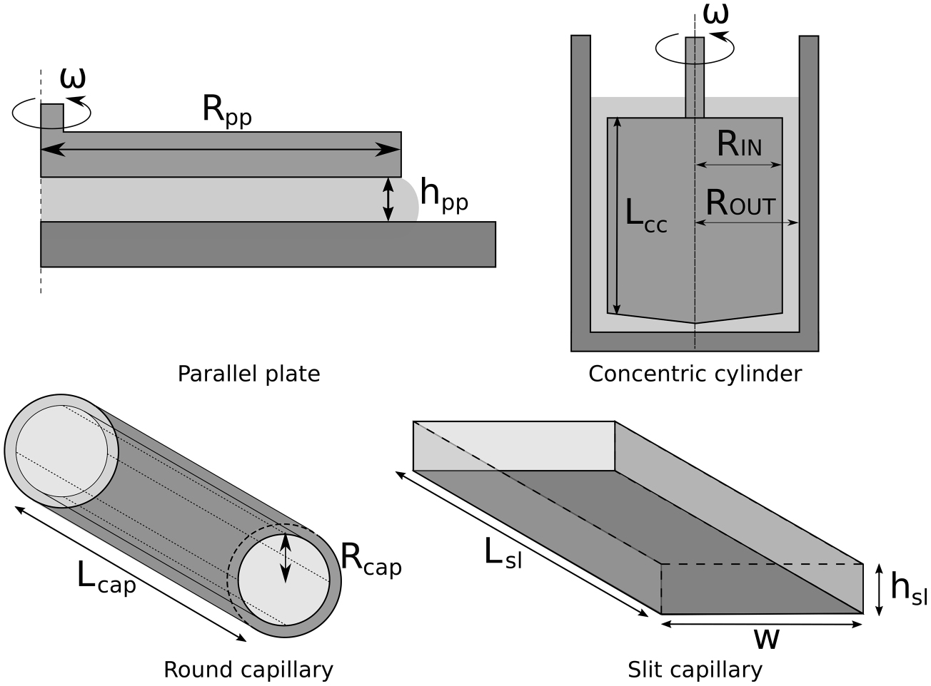
The geometrical definition of these rheometer are given in figure 1 and will be used throughout the paper. The cone plate is left out as it has a similar but smaller measuring range as the parallel plate and is less suited for measuring high shear rates.

Figure 1. Geometrical definitions.
Download figure:
Standard image High-resolution imageThe goal of the measuring device is to determine the rheological properties of a fluid. The viscosity is determined by applying a velocity and measuring the force or torque required or vice versa. These are converted through a model into the viscosity. The model assumes the following conditions for the measurement.
- 1.Unidirectional shear
- 2.Laminar flow
- 3.Wall adherence
- 4.Isothermal flow
- 5.Incompressible flow
Once the assumptions are untrue, errors enter the measurement. Each model assumption is discussed and its limitation derived.
2.1. Unidirectional shear
Unidirectional shear means that no secondary flows are present. At high shear rates the measured fluid is moving at high speed. As long as the viscous force is dominant over the centrifugal force the flow is unidirectional. However, once this is no longer true, the fluid starts moving outwards and unwanted flows occur. This inertial effect is present in all rotational devices, although there is a difference in how the rheometers counteract this inertial effect and thus what range they can measure before the effect dominates the measurement.
2.1.1. Parallel plate.
In the case of these rotary measurement methods the flow towards the outside is the first occurring secondary flow. At one plate the fluid will flow from inside to outside and at the other reversed. The secondary flow is initially laminar but can become turbulent. A dimensionless number can be formed describing the onset of secondary flows [25], according to the following analysis. The secondary flow is characterised by the forces acting on a unit volume. The forces acting on this unit can be evaluated in a steady state in the radial direction. The dimensionless number  is created to give the ratio of these forces, equations (1) and (2). Geometrical definitions for parallel plate from figure 1 are used. The
  number is the Reynolds number in the radial direction.
When the critical  number is exceeded, secondary flows will occur which results in a higher measured viscosity. In particular non-Newtonian fluids will show complex behaviour as the increased shear stress will alter the viscosity. The critical value of the
  number for cone-plate and parallel plate is 6 according to [25].
At the edges of parallel plate measuring geometry, the forces on the unit volume are different. As these devices have open edges the centrifugal force is countered by the surface tension. There is the possibility that the centrifugal force overcomes the surface tension. This phenomenon, known as radial migration, limits the range of the rheometer, equation (3) [26]. The balance between the surface tension and the inertial forces results in a critical shear rate. This critical shear rate is fluid dependent and strongly dependent on the gap height. The equation for the critical shear rate can be found in equation (4) [26]. Geometrical definitions for parallel plate from figure 1 are used.
The result of radial migration can be seen as a drop in measured torque. As there is less fluid, the shear stress is reduced. Repeating the measurement will result in lower torques measured due to the loss of fluid and thus a lower viscosity is measured.
2.1.2. Concentric cylinder.
As with the parallel plate rheometers, the concentric cylinder is influenced by the centrifugal forces in the fluid. However, due to the fluid being held inside by the outside cylinder, the fluid cannot be flung out. A rising pressure gradient occurs between the inner and outer cylinder. This balance is not stable and when the rotational speed exceeds a certain point, secondary flows occur. This phenomenon was first studied by Geoffrey Ingram Taylor in 1923. Through dimensionless analysis a quantification of the relation between viscous forces and the inertial forces was described. He found the critical Taylor number at which Taylor vortices occur. The Taylor number is defined in equation (5) [27, 28]. Geometrical definition from figure 1 for concentric cylinder are used.
When increasing the angular velocity even further, different Taylor vortices occur. The Taylor vortices are initially laminar flows. The increased shearing in the fluid results in a higher torque measured and thus higher viscosities measured. For non-Newtonian fluids the extra shear affects the viscosity in the fluid. The critical Taylor number that defines the first occurrence of the vortices is 1700 [28].
2.2. Laminar flow
Laminar flow is required to generate a well-defined flow profile. The flow profile is used to determine the shear rate in the fluid. As the speed of the fluid increases, the laminar flow transitions into turbulent flow. Turbulence occurs due to layers of fluid moving at different speeds. Turbulence has been studied for many types of pipe flow. The capillary devices are pipe flows and therefore are limited to the onset of turbulence which can be expressed by a critical dimensionless Reynolds number. The Reynolds number is used to quantify the balance between inertia forces and the viscous forces. The Reynolds number is defined in equation (6).
For the capillary devices the Reynolds number is transformed in different shape specific equations, equations (7) and (8). Geometrical definition from figure 1 for round capillary and slit capillary were used respectively. Turbulence creates extra shear stress in the fluid and chaotic flow. This increases the friction and results in higher viscosities measured. The critical Reynolds number defines the limit of the laminar flow.

Turbulence occurs in the rotational devices as well, although it forms after the instabilities discussed in the previous section. The Reynolds number is proportional to the speed of the fluid. This means turbulence starts occurring at the edges of the rotational devices.
2.3. Wall adherence
A key assumption is the zero wall slip condition. This condition states that fluid in contact with a wall does not move along the wall. In reality, this is not always true. When the cohesion forces are stronger than the adhesion forces the fluid is pulled along the walls. When wall slip occurs the flow profile is changed, figure 2. The true shear rate is lower than the apparent shear rate the model assumes. Therefore the viscosity is underestimated.
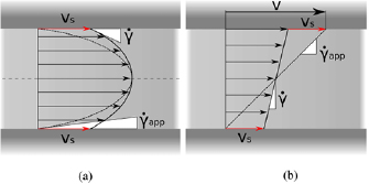
Figure 2. Effect of wall slip on the flow profile. In red the slip velocity. (a) Wall slip pressure driven flow. (b) Wall slip Couette flow.
Download figure:
Standard image High-resolution imageDepending on the fluid and for example the wall material, slip can occur. Slip can also be caused by other factors such as wall depletion, i.e. larger particles are pushed out of the boundary layer. The smaller particles then form a lubricating layer along the walls. The shearing is then mostly limited to the boundary layers, figure 3.

Figure 3. Wall depletion in suspensions.
Download figure:
Standard image High-resolution imageCorrections for wall slip have been developed since 1931 by Mooney. The Mooney analysis is applicable to all the analysed devices [29].
The slip will not be taken into account in the determination of the measuring range as it is fluid and material dependent. Furthermore, current rheometers do not correct for wall slip.
2.4. Isothermal flow
In general, the viscosity of a fluid is strongly temperature dependent. Most rheometers are temperature controlled to either measure or negate this temperature dependence. As the shear rates increase at constant forcing more energy is put into the fluid. All of this energy is converted into heat. This heat is dissipated through the fluid and eventually transferred to the outside world or absorbed by the fluid increasing the fluid temperature. As the viscosity of a fluid is temperature dependent this heating of the fluid must be avoided. When the temperature starts influencing the viscosity the momentum equation of the Navier–Stokes equation becomes coupled to the energy equation making the prediction of the fluid flow complicated. An indicator for the significance of the heating of the fluid is given by the dimensionless Nahme–Griffith number [30]. This number is the ratio between heat generation inside the fluid over the dissipation of the heat. As long as more heat is dissipated than generated due to viscous friction the effect is negligible. The Nahme–Griffith number is closely related to the Brinkman number which is used to quantify the effect a certain temperature change has on the viscosity. The formulas for the Nahme–Griffith number of the different rheometers types can be found in table 2.
Table 2. Table showing the Nahme–Griffith number for different types of rheometers [30], geometrical definitions from figure 1.
| Rheometer | Nahme–Griffith |
|---|---|
| Na = | |
| Parallel plate |  |
| Concentric cylinder |  |
| Slit capillary |  |
| Round capillary |  |
When viscous heating is present, the viscosity is locally lowered. The measured viscosity is therefore reduced. In literature, a Nahme number of 1 is seen as the limit [31].
2.5. Incompressible flow
The compressibility of the fluid flow has an effect on the measurement of the viscosity. The model assumes the viscosity is not a function of the pressure. Most fluids can be considered incompressible. In reality, the pressure does influence the viscosity, however, this effect is limited. The pressure dependence of the viscosity for water at different temperatures is presented in [32] and is 
 Pa s MPa−1 to
 Pa s MPa−1 for a temperature range of 0 °C–25 °C. For lubricating oils the pressure dependence of the viscosity is larger, but it may still be neglected at the low pressure levels expected in the rheometers discussed in this study. The capillary rheometers will be more influenced by this assumption as they introduce a pressure difference to function, although, this effect is still negligible.
2.6. Pressure/speed limits
The system requires sensors and actuation. These have their limitations. These sensor maximum and minimum can be translated into a maximum and minimum viscosity at a given shear rate. These limitations create operation boundaries. Similarly, the actuation will have a limit defining a maximum and minimum attainable shear rate. Table 3 presents the equations used to find the limits of the analysed devices. By inserting the measuring range of the sensor in to the formula a maximum and minimum measurable viscosity is calculated for a given shear rate. By inserting the actuation range of the actuator in to the formula a maximum and minimum attainable shear rate is calculated.
Table 3. Equations defining the max-minimum viscosity at a given shear rate due to the sensor and max-minimum shear rate due to actuation limitations. Geometrical definitions from figure 1.
| Rheometer | Limit due to sensing | Limit due to actuation |
|---|---|---|
 |
 |
|
| Parallel plate |  |
 |
| Concentric cylinder |  |
 |
| Slit capillary |  |
 |
| Round capillary |  |
 |
2.7. Comparison
Taking into account all the discussed limitations in the previous sections, the working area of the measurement principles can be predicted. This gives the ability to determine the working range of different rheometer types. The free geometrical variables are listed in table 4.
Table 4. Variables in de measurement systems, geometrical definitions from figure 1.
| Device | Variable |
|---|---|
| Parallel plate |  |
 |
|
| Concentric cylinder |  |
 |
|
 |
|
| Slit capillary |  |
| w | |
 |
|
| Round capillary |  |
 |
|
The goal of the analysis is to compare the working principles to make a choice for the best design in a specific case. Therefore, the measuring methods have to be linked together. A way to do this is to match a characteristic dimension. In this case the characteristic length should be related to the shearing of the fluid. A re-occurring parameter in table 4 is the gap height. By linking the height of the gap, a link is made between the devices on the space where the shearing takes place.
The gap heights of the parallel plate, concentric cylinder and the slit capillary can be matched. This leaves the round capillary. The round capillary can be matched with the slit capillary through the hydraulic diameter, equation (9).
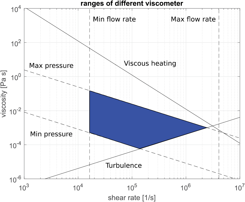
As an example the measuring range is calculated for a slit rheometer measuring kerosene, figure 4, with measuring length: 1 mm, gap height: 50  m, width: 0.5 mm, maximum pressure: 4 MPa, minimum pressure: 10 kPa, maximum flow rate: 25 ml min−1 and minimum flow rate: 100
  l min−1.

Figure 4. Example of the measuring range for a slit rheometer.
Download figure:
Standard image High-resolution imageIn figure 4 the different limitations discussed in previous sections are put together to define the theoretical measuring range. Turbulence from section 2.2. Viscous heating from section 2.4. The maximum/minimum pressure and shear rate from section 2.6. Depending on the geometrical dimensions chosen the theoretical measuring range can be determined.
The limits of each measuring principle as defined in section 2 have been applied and the measuring ranges defined for a common characteristic of 35  m as defined in section 2.7. An overlay of the theoretical ranges can be found in figure 5. The fluid properties of kerosene are used in the measuring ranges.
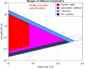
Figure 5. Theoretical ranges of the measurement principles for a gap of 35  m.
m.
Download figure:
Standard image High-resolution imageFrom figure 5 we can see that the capillary devices have a slight advantage in measurement range. Moreover, both capillary devices are less influenced by viscous heating. The Nahme–Griffith number describes the viscous heating at a specific shear rate. Pressure driven flows have a varying shear rate over their gap, where the shear rate is highest at the edges. For concentric cylinder devices the shear rate is nearly constant over the gap. When this shear rate is high enough to cause viscous heating, the entire fluid is heating up. Additionally, the capillary devices continuously introduce new fluid to the system whereas the rotational devices reuse the fluid which could already have been affected by viscous heating. Thus intensifying the heating of the fluid. Lastly, capillary devices have an advantage in the application of a homogeneous magnetic field due to the linear shape.
The capillary concept, therefore, best fulfils the requirements. Within this group, the slit capillary concept is chosen due to the fact that producing rectangular microchannels is more cost effective and can be done more consistently.
3. Design of measuring geometry
Firstly, the current commercially available and research magnetorheometers are analysed. Secondly, the non-magnetorheometers are analysed for their characteristics in order to determine the requirements for a new rheometer. The requirements can be found in table 5. These requirements are set as a target for the new design.
Table 5. Requirements.
| Shear rate | 106 | s−1 |
|---|---|---|
| Magnetic field density | 1 | T |
| Repeatability | 2 | % |
| Accuracy | 2 | % |
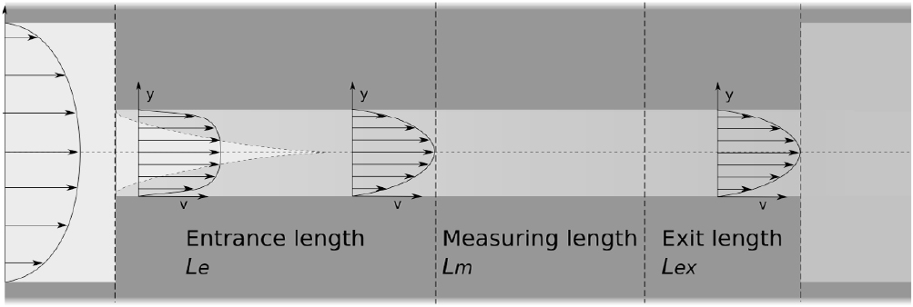
A slit capillary consists of three parts: the entrance length, the measuring length and the exit length, figure 6.
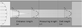
Figure 6. Channel design.
Download figure:
Standard image High-resolution imageThe entrance length is needed to create a fully developed flow and should be sufficient for the lowest viscosity fluid targeted. The transition to turbulent flow on macro scale is seen as a Reynolds number of 2300. In literature the transition phase for microfluidics is however still disputed. The consensus is that it does not start before a Reynolds number of 1000 [33]. To accommodate the fluid entering and stabilising, an entrance length is determined by equation (10) [34].
The measuring length is 1 mm as this creates a measurable pressure drop for low viscosity fluids while not requiring an excessive feed pressure for higher viscosity fluids. The exit length is 0.2 mm. Increasing the exit length increases the required inlet pressure. However, by extending the exit length the magnetic fluid can be drained more easily from the channel.
Lastly, the gap height needs to be determined. A lower gap height results in higher shear rates, lower viscous heating and an increase in the required inlet pressure. The goal is to measure rheological properties magnetic fluids. This means the gap height must be large enough to allow the magnetic particles through and form chains to create the magnetorheological effect.
The particle size for MR fluids are around 1  m, therefore a lower limit of 20
  m is set to allow for chains of more than 10 particles to form [35].
Through an iterative process of weighing the pressures required to drive the fluid and the heat generation, a gap height of 35  m was chosen. This results in the following measuring range for kerosene, figure 7.

Figure 7. Working range of designed rheometer.
Download figure:
Standard image High-resolution imageThe maximum shear stress to be measured is tuned to have a Nahme–Griffith number of 1 at 106 s−1 which results in a pressure at the entrance of the channel of 4 MPa, equation (11) [30]. The parameter values can be found in table 6 and figure 8.
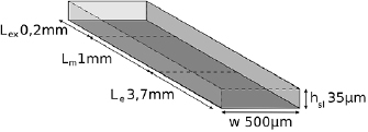
Figure 8. Final dimensions of the channel.
Download figure:
Standard image High-resolution imageTable 6. Final pressures at different locations of the channel.
| Parameter | Value (MPa) | |
|---|---|---|
| Inlet pressure |  |
4 |
| Sensor pressure high |  |
0.90 |
| Sensor pressure low |  |
0.15 |
The width of the channel has a lower limit. Edge effects of the side walls are negligible when the width is at least 10 times the gap height [36, 37]. The width of the channel has limited effect on the range but determine the flow rate. By tuning the width of the channel, the flow rate is adjusted to combine it with the flow rate of the pump, equation (12).
The magnetic core was designed to apply a homogeneous and uniform field over the microchannel. The choice was made to use a symmetric design to create this homogeneous field. The field has to be concentrated on the small area of the channel. The size on the pole piece was made four times as large as the channel dimensions. A 3D simulation of the magnetic field showed negligible variation of the field density over the microchannel. The coil geometry was determined using the magnetic reluctance [38]. The final parameters used can be found in table 6 and figure 8. The design of the core is presented in figure 18.
The simplest design would be to have the pressure sensors directly next to the channel, however, due to the magnetic core which surrounds the channel, there is limited space. Therefore, sensor channels are created, figure 9. The sensor channels have to be much wider than the channel in order not to create significant pressure drop to the pressure sensors.

Figure 9. Design assembled slit.
Download figure:
Standard image High-resolution imageThe final design can be seen in figure 10 with the layers numbered. This results in a multi layered design where in the second layer the sensor channels are cut out. The third layer seals the sensor channels and allows for connectors to be mounted. A forth layer is added to create more connecting length for the connectors and make them more robust.
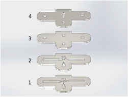
Figure 10. Exploded view of chip design in layers.
Download figure:
Standard image High-resolution imageTo show the functioning of the designed rheometer, a prototype is manufactured. This prototype uses a syringe pump with a maximum pressure of .67 MPa and a maximum flow rate of 25.99 ml min−1. This limits the measuring range. The range can be seen in figure 11.

Figure 11. Prototype working range limited due to used syringe pump pressure limits.
Download figure:
Standard image High-resolution imageThe range in figure 11 is limited by the syringe pump used, however, does reach the desired high shear rates.
4. Fabrication
For the fabrication of the entire device 3 subsystems have to be built. Firstly, the microchannel itself. Secondly, the magnetic system and finally the external systems such as data acquisition and the pump.
4.1. Microchannel fabrication
The fabrication of the micro device is complicated. Most micro devices are made through a chemical etching process, however, this is expensive and time consuming. In microfluidics, hot embossing techniques have been developed for quick prototyping [39]. Hot embossing uses a master design to press features into a plastic substrate. This process has been chosen in order to make devices in a cost effective manner. The substrate material chosen is Poly(MethylMethAcrylate), (PMMA). PMMA was chosen as it is a cheap material, has a high stiffness, is transparent and easily moulded [40]. The fabrication process for the chip consists of five steps.
- 1.Master production
- 2.Hot embossing
- 3.Flattening
- 4.Bonding
- 5.Final assembly
4.1.1. Master production.
A laser etching machine is chosen to etch the master design in silicon. The laser is a Spectra Physics Q-switched Talon laser 355-15 with maximum output of 15 W at 50 kHz repetition frequency and with 13 W at 100 kHz. The maximum frequency is 500 kHz with a pulse width of 35 ns. Different laser patterns and rotations have been tested to optimize the height differences created by the laser path. The best result was obtained by laser etching the silicon with a 5  m line spacing in a net pattern. The etch is repeated once with a 45° rotation of the net etching pattern. A firing rate of 20 kHz with a laser speed of 20 m s−1 was used [41]. The produced master is cleaned in Isopropanol with an ultrasonic cleaner for half an hour, then spincoated with a anti stiction monolayer, EVGNIL ASL for releasing the PMMA after the embossing process, figure 12.
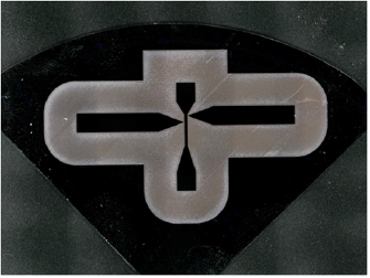
Figure 12. Silicon master.
Download figure:
Standard image High-resolution image4.1.2. Embossing.
The master is placed in a mechanical press and covered with a piece of 1 mm thick PMMA cut into the shape of the chip design. The PMMA is covered with a silicon wafer to improve the surface roughness of the counter surface.
The assembly is clamped between two sheets of aluminium and two cast steel plates and tightened by four bolts, figure 13. The bolts are hand tightened and the assembly placed in an oven preheated to 145 °C for 20 min. The bolts are then tightened with a torque wrench to an overall pressure of 0.9 MPa. The assembly is left in the oven for 20 min, then slowly cooled to 110 °C in about 20 min. The pressure is removed and the press is disassembled. The master is separated from the PMMA and left to cool to room temperature. The temperature and pressure are sketched in figure 17 as the solid lines. The embossing procedure is taken from [42] and adapted through trial and error to get the best results for the used equipment. The embossed PMMA can be seen in figure 14.
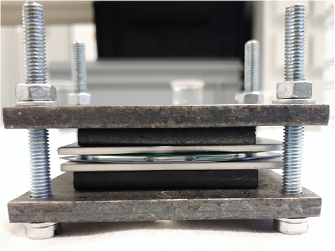
Figure 13. Assembled press.
Download figure:
Standard image High-resolution image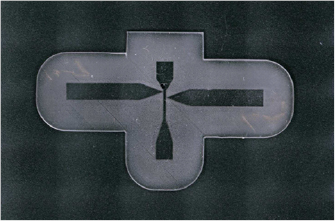
Figure 14. Embossed PMMA.
Download figure:
Standard image High-resolution image4.1.3. Flattening.
The uneven surface on the PMMA, due to the laser etched surface, is subjected to flattening stages. As a result of these steps, the bonding is improved and a sealed microchannel is obtained. The PMMA is put in between two layers of silicon and assembled in the press. A pressure of 0.57 MPa is applied. The assembly is put in a preheated oven at 110 °C for 55 min and then cooled under pressure to room temperature. The improvement of the bonding surface can be seen in figure 15. The flattening process does have an effect on the channel geometry. Due to the temperature and pressure the channel swells slightly.
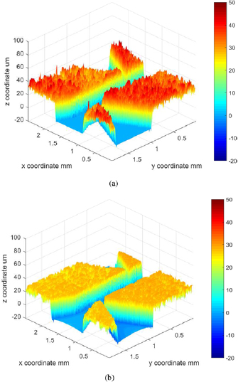
Figure 15. White light interferometry images of PMMA surface before (a) and after (b) the flattening process. (a) Before flattening. (b) After flattening.
Download figure:
Standard image High-resolution image4.1.4. Bonding.
The bonding step is similar to the embossing step but requires a lower temperature to inhibit deformation of the geometry. Layers 2, 3 and 4, figure 10, are aligned and assembled in the press. For a smooth counter surface, silicon wafers are placed on either side. The press is tightened to 0.57 MPa and placed in an oven preheated to 110 °C. The assembly is left in the oven for 90 min and then slowly cooled to room temperature. The pressure is removed and the press is disassembled.
The bond of the embossed PMMA to the bonded layers 2–4, figure 10, is done chemically [43]. A solution of 70% Isopropanol is distributed on top of the embossed PMMA. The remaining layers placed on top. The assembly is pressed together and the excess solution is removed. While under slight pressure the layers are aligned using alignment tools. The press is hand tightened and placed in a preheated oven of 68 °C. The press is left for 15 min. The press is removed and slowly cooled to room temperature. Once cooled the pressure is removed. The temperature and pressure are sketched in figure 17 as the striped lines and dotted lines as thermal bonding and chemical bonding respectively. The final assembled chip can be seen in figure 16.
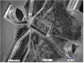
Figure 16. The assembled chip.
Download figure:
Standard image High-resolution image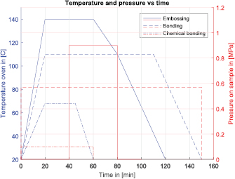
Figure 17. Embossing, bonding and chemical bonding process parameters. Temperature in the oven and pressure on PMMA against time.
Download figure:
Standard image High-resolution image4.2. Magnetic system
A magnetic core has been designed to apply the 1 T field on the microchannel. The core has been fabricated from St37 steel. The core has been designed as a layered design to be able to laser cut and assemble the core. The coils have a diameter of 30 mm and are wrapped with 400 windings of 0.55 mm diameter magnetic copper wire. The gap is 3 mm to allow for the microchannel to be placed in between. The fabricated core can be seen in figure 18.
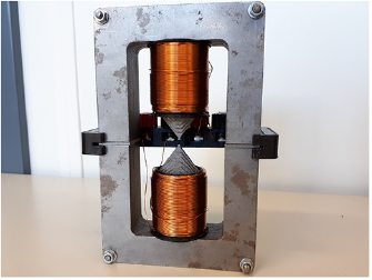
Figure 18. Fabricated core.
Download figure:
Standard image High-resolution imageThe magnetic behaviour has been characterised at the location of the microchannel using a Gauss meter. The current has been varied from  A to 3 A whilst measuring the magnetic field density, figure 19.
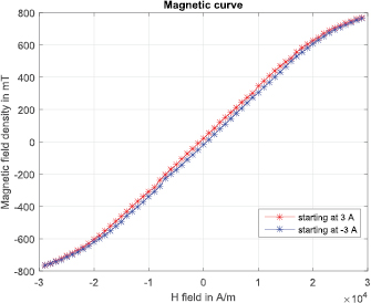
Figure 19. Magnetic field strength curve at microchannel in air.
Download figure:
Standard image High-resolution image4.3. Final assembly
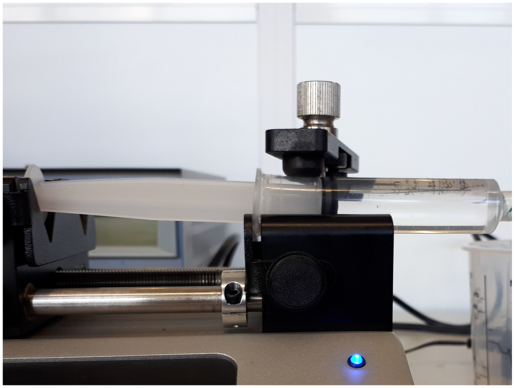
The PMMA assembly needs to be connected to the supply pump and sensors. The connectors are adapted Festo straight barbed 3 mm connectors. One side is filed down to 3 mm diameter. The connections are glued in place with Bison plastic epoxy. The Festo piping connects the PMMA to the pressure sensors and the syringe pump. The test setup can be seen in figure 20.
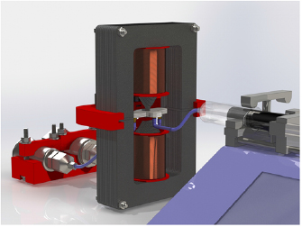
Figure 20. Test setup.
Download figure:
Standard image High-resolution image4.4. Sensors and data acquisition
The pump being used is a Kd Scientific Legato 111 double syringe programmable infusion and withdrawal pump. The syringe used is a 10 ml plastic Terumo syringe. The pump has a maximum flow rate with this syringe of 25.99 ml min−1 which is sufficient to reach shear rates over 106 s−1.
5. Measurement procedure
Figure 21 shows a typical measurement. The measurement is started in steady state with zero flow. By taking 100 samples points a zero measurement for the sensors is made. After these, a starting flow rate is applied. Once the measured pressure has reached a steady state the flow rate is increased. This process is repeated until the syringe is empty. As the flow is stopped the pressures quickly return to their zero value.

Figure 21. Typical measurement of pressure against time at different flow rates with deionized water.
Download figure:
Standard image High-resolution imageThe measured pressures and flow rates are converted into shear stresses and shear rates through the geometrical model, equations (11) and (12), respectively.
6. Results
6.1. Preliminary test
The seal of the microchannel is tested through two simple tests. Firstly the chip is submerged in water for a leak test. Air is pressed into the channel through a syringe. The air bubbles appearing show the flow of air and the leakages.
In the second test water is pressed into the chip with a syringe. The meniscus moving through the chip can be perceived, showing that the fluid does not flow in between the layers.
6.2. Results
The results are plotted in figures 22–24.
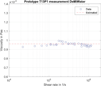
Figure 22. Viscosity of deionized water at high shear rates.
Download figure:
Standard image High-resolution image
Figure 23. Viscosity of Shell Tellus S2 VX15 at high shear rates.
Download figure:
Standard image High-resolution image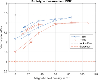
Figure 24. Viscosity of magnetic fluid with different magnetic fields at a constant shear rate.
Download figure:
Standard image High-resolution image6.2.1. Deionized water.
The resulting viscosities at different shear rates are compared to the viscosity of deionized water at 21.8 °C, 0.96 mPa s [44]. The maximum shear rate measured was  s−1. Higher shear rates were not measured as the pump engine stalled.
The chip was cleaned and filled with Shell Tellus S2 VX15. The resulting viscosities can be seen in figure 23. The expected viscosity is taken from the data sheet provided by Shell. The expected viscosity is 23 mPa s. The measurements from the Anton Paar rheometer have been added.
Lastly, Ferrotec EFH1 has been measured to show the magnetorheological effect. The relation between magnetic field and the current steps was measured to be able to translate the current into magnetic field density. In figure 24 the flow rate was kept constant over the entire measurement,  s−1. The current was increased in steps and then reduced. The resulting pressure rise translates into an increase in viscosity, showing the magnetorheological effect. The resistance to flow has increased due to the magnetic field.
7. Discussion
Firstly, a measuring principle was determined. After a comprehensive comparison of pertinent rheometer concepts, the slit capillary rheometer was selected as the most promising concept. It was chosen because of its high measuring range compared to other rheometer types, the simple application of the magnetic field and its low viscous heating effects. This concept was further developed into a detailed design for a prototype. Fabrication techniques were found and used to build the prototype. The resulting prototype succeeded in measuring deionized water, figure 22, Shell Tellus S2 VX15 oil, figure 23, and Ferrotec EFH1 and showed the magnetorheological effect, figure 24.
7.1. Low pressure sensor
In the prototype a misalignment was introduced, effectively reducing the exit length of the slit. The misalignment is created during the chemical bonding of layers 1 and 2, figure 10. A closer look at the misalignment is given in figure 25. The exit length was dimensioned to be 0.2 mm but is measured to be 0.02 mm. This results in reduced pressures measured at the sensors. This brings the measured signal at the low pressure sensor in the noise range. The misalignment can be prevented by adding alignment features to the design. The results in this paper have been corrected for this error by using the actual exit length, not the designed exit length.
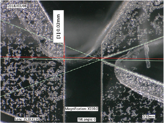
Figure 25. Misalignment influencing the measured low pressure.
Download figure:
Standard image High-resolution image7.2. Experimental setup
7.2.1. Maximum shear rate.
The maximum shear rate measured is  s−1, figure 22. No higher shear rates were measured as the syringe pump motor stalled. This means the maximum pump pressure was applied to the chip. The expected pressure at the entrance for the maximum shear rate measured is 0.44 MPa, whereas the maximum pressure produced by the pump is 0.67 MPa. This means this pressure is lost between the pump and the sensors. Further analysis revealed that this is caused by a restriction in the channel entrance. The restriction has two sources: the channel swelling in the flattening stage and the misalignment between layers 1 and 2, figure 10.
As layer two is closer to the swelling of the channel (blue in figure 26), the entrance becomes much smaller than designed and causes an increased pressure drop. The swelling of the channel could be prevented by removing the flattening stage, section 4.1.3. This means improving the master such that the bonding surfaces are smooth. The swelling at the entrances does not affect the accuracy of the measurement but restricts the maximum shear rate reached with the maximum pressure of the syringe pump.
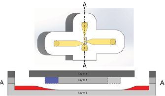
Figure 26. Entrance restriction, channel swelling in red, misalignment in blue.
Download figure:
Standard image High-resolution image7.2.2. Response time.
As a step in the applied flow rate is initiated, a delay (d) is noticed in the pressure response. After this delay the pressure rises steadily and stabilises to a pressure, figure 27. The delay is primarily caused by air bubbles in the syringe. The air in the syringe is compressed as the pressure increases, reducing the applied flow rate temporarily. After this initial delay the measured pressure increases, although not instantly as the incompressibility assumption would suggest. The slow response, ( ), is caused by the type of pressure sensors used. The sensors have a membrane which deforms due to the applied pressure. The deformation is measured and converted into a pressure. Due to the incompressibility, the deformation of the membrane means an increase in the volume in the sensor channel. This volume has to be filled with fluid from the measuring channel to increase the measured pressure. The limited access to the measuring channel creates a flow restriction which causes the slow response of the measured pressure.
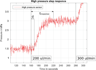
Figure 27. High pressure response to flow rate step increase.
Download figure:
Standard image High-resolution imageThe delay can be prevented by draining the air bubbles from the system before measuring. The pressure response can be accelerated by having smaller measuring membranes in the sensors or increasing the stiffness of the membrane. This reduces the volume flow required for the pressure to increase. A further improvement would be to reduce the restriction to the measuring channel.
7.2.3. Blockages.
Some measurements failed due to blockages in the microchannel. It is critical to keep the system clean as the microchannel is a mere 30  m in height. This issue was encountered with the first measurement using magnetic fluids. Due to the misalignment and swelling of the channels the effective gap was reduced significantly at the entrance. The entrance became blocked by the particles bridging across the channel [45]. The blockage increased the pressure drastically at the entrance causing a leak of the chip. The entrance geometry can be improved to reduce the formation of particle bridges. The tapered entrance strengthens the bridges that are formed. Therefore a sharp entrance is preferred.
7.2.4. Syringe.
Due to the high flow rates required and the restriction in the flow path, the maximum force is applied to the syringe. After the high shear measurements it was perceived that the syringe had deformed due to the applied force. The fixation of the syringe pump is not able to hold the syringe in place, figure 28.

Figure 28. Deformation of the syringe due to high pressure in the system.
Download figure:
Standard image High-resolution imageThis results in a slightly lower flow rate being applied to the chip which means lower pressures are being measured. During the data processing this results in lower viscosity due to the flow rate used in calculation is higher than in reality. The deformation can be prevented by using stainless steel syringes, creating a custom fixation for the syringe pump or using a different pumping concept.
7.2.5. Sensor zeroing.
Before each measurement the pressures at zero flow rate were measured. The data is corrected during the data processing for the non-zero pressure at zero flow. The non-zero values are due to the gravitational force of the fluid in the connection tubes to the sensors and the offset of the sensors. However, due to the restriction in the sensor channels and surface tension of the measured fluid, the pressure did not always reach the true zero pressure value. The sensor channels were able to keep an over or under pressure. Once the flow was initiated the flow would correct itself.
7.2.6. Gap height.
The gap height is only known before the chemical bonding. As the channel swells about 2  m, the exact gap height is slightly varying over the channel, figure 29. The gap height is therefore slightly altered to fit the deionized water measurements. The alterations are less than 2
  m. Once the parameter is set it is not altered for any other measurement.

Figure 29. XZ view of T13P1 showing the channel swell.
Download figure:
Standard image High-resolution image
7.3. Discussion measurements
The highest deviation for the water measurement after geometrical corrections is less than 8% for deionized water and Shell Tellus VX15 oil. The maximum shear rate measured is  s−1. The measurements with Ferrotec EFH1 show the device is able to measure the magnetorheological effect. This means that this prototype can be expanded into the measuring of larger particle magnetic fluids at high shear rates. To be able to perform these measurements some improvements will be necessary. Currently the system is not strong enough to withstand the pressures involved with measuring MR fluids at high shear rates as the viscosity of MR fluids are higher.
8. Conclusions
From the physics based analysis of the measuring principles, it follows that capillary devices have an advantage in measuring magnetic fluids as they can reach higher shear rates while at the same time simplifying the application of a magnetic field. The measurement has a maximum deviation of 8% compared to the true viscosity. The viscosity is measured to a shear rate range of 104 s−1– s−1.
s−1.
The measurement on the magnetic fluid clearly show the influence of the magnetic field on the rheology of the fluid. More experiments should be performed with the designed rheometer on magnetic fluids to fully capture the potential of the device.
The final conclusion of this paper is that we can say that we have successfully designed and built a prototype of an ultra high shear rheometer capable of measuring magnetic fluids and a range of 104 s−1–106 s−1.