

Abstract
We analyze changes in the maximum annual transient snowline elevation (MATSL) of glaciers for two regions in western North America from 1984 to 2024 using five satellite remote sensing datasets. MATSL reached its highest elevations in 2019 (155 m above the long-term average) for Alaska (Region 1) and in 2023 (148 m) for Western Canada and USA (Region 2). The rate of MATSL rise accelerated fourfold, increasing from 2.1 ± 0.8 m a−1 in 1984–2010 (r2 = 0.1, p < 0.01) to 8.9 ± 1.7 m a−1 in 2010–2024 (r2 = 0.5, p < 0.01). In 2019, 91 glaciers exceeded the 95th percentile MATSL elevation, a threshold indicative of complete loss of the accumulation area, in Region 1. In Region 2, 149 glaciers exceeded this threshold in 2023. Year-to-year variability in MATSL was strongly influenced by mean summer air temperature with sensitivities of +46 m °C−1 (r2 = 0.54) and +23 m °C−1 (r2 = 0.30) for Regions 1 and 2, respectively. Mean spring snow water equivalent also played an important role with sensitivities of −351 mm w.e.−1 (r2 = 0.48) and −155 mm w.e.−1 (r2 = 0.37), respectively. Per-glacier analysis revealed that south-facing slopes experienced the largest MATSL increases. Terrain attributes, including slope, aspect, hypsometry, and elevation, enhanced MATSL prediction models compared to those using only climate variables. The pronounced rise in MATSL underscores a critical glacier melt feedback mechanism, warranting further investigation. This study highlights the utility of automated MATSL time-series mapping for regional-scale analyses and identifies key limitations and opportunities for future research.

Original content from this work may be used under the terms of the Creative Commons Attribution 4.0 license. Any further distribution of this work must maintain attribution to the author(s) and the title of the work, journal citation and DOI.
1. Introduction
Mountain glaciers are integral components of the hydrological cycle and are particularly sensitive to anthropogenic climate change (Moore et al 2020, IPCC 2023). Globally, glaciers are experiencing rapid mass loss, primarily driven by rising air temperatures (Hugonnet et al 2021). This trend is also evident in western Canada, where glacier area loss accelerated starting in 2010 (Bevington and Menounos 2022). This decline is compounded by a thinning and darkening snowpack, along with shorter winter seasons, which exacerbate the glaciers' negative mass balance (Najafi et al 2017, Bertoncini et al 2022). The continued glacier loss is expected to alter the timing and volume of freshwater in rivers, leading to societal and ecological impacts (Benn and Lehmkuhl 2000, Huss and Hock 2018, Chernos et al 2020, Pitman et al 2021).
Remote sensing provides a valuable tool for monitoring glacier changes on seasonal to interannual timescales (Tennant et al 2012, Pelto 2019). Additionally, mapping snow on glaciers using satellite imagery enables the analysis of intraseasonal changes in snow accumulation (Pelto 2011, Rastner et al 2019), which in turn allows for the calculation of the snowline elevation, also known as the transient snowline elevation (TSL). The annual maximum TSL (MATSL) is a strong indicator of glacier mass balance (Østrem 1974, Benn and Lehmkuhl 2000, Lorrey et al 2022).
While some large-area MATSL mapping studies exist, most rely on manual threshold classification of satellite imagery, limiting their scalability across large regions or over extended time periods (Larocca et al 2024). To our knowledge, MATSL mapping for all western North America has not been systematically analyzed or published.
This study maps the MATSL and quantifies its change in western North America over the period 1984–2024 (figure 1). Specifically, we focus on: (1) examining spatial patterns of MATSL change and identifying the climatic drivers of variability, and (2) evaluating recent MATSL trends in the context of a longer observational record.
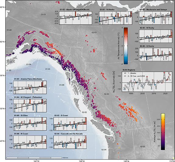
Figure 1. Map of the study area, including RGI Regions 1 (Alaska) and 2 (Western Canada and USA), and RGI sub-regions (dashed white lines). The main map panel shows the per glacier average MATSL elevation (m asl) over the study period (1984–2024). Sub-panel 'Both Regions' shows the average regional MATSL anomaly (in meters) over the period of record for Regions 1 and 2. The bars are colored by the mean summer air temperature (MSAT) anomaly over the glaciated area of each region. Sub-panels for each RGI Sub-region share the same x-axis labels as the 'Both Regions' sub-panel. Note: the westernmost extent of sub-region 01–03 is not included due to insufficient imagery in the 1980s and 1990s.
Download figure:
Standard image High-resolution image2. Data and methods
2.1. Glacier polygons
Glacier polygons from the Randolph Glacier Inventory (RGI) Version 7 (Pfeffer et al 2014) serve as the basis for this analysis of Alaska (RGI Region 1) and Western Canada and USA (RGI Region 2) (figure 1). This dataset includes 46,239 glaciers, covering 101,229 km2. Over 95% of the outlines originate from satellite imagery captured between 2004 and 2010, with the latest outlines from 2011. Although updated glacier outlines exist for British Columbia and Alberta (e.g. Bevington and Menounos 2022), they do not encompass our entire study area. To reduce edge effects and shadows, glaciers smaller than 2.0 km2 are excluded from the study, along with 14 poorly digitized high elevation snowfields that lack ablation zones. These exclusions result in 4456 glaciers remaining, representing 84.5% (85,579 km2) of the total glaciated area.
2.2. Satellite imagery
Optical satellite imagery from 1984 to 2024 is used in this analysis, including five calibrated surface reflectance collections from the Landsat and Sentinel-2 programs with 20–30 m spatial resolution (table 1). Images acquired from July to September with <20% cloud cover in their metadata are kept. Each year, glaciers are, on average, imaged twice before the year 1999 and 12 times after 2019 (supplementary figure 1). Imagery is processed using the 'rgee' R package, which interfaces with Google Earth Engine (GEE) (Gorelick et al 2017, Aybar et al 2020). Cloud masks included in these collections perform poorly over glacier margins, and thus we include clouds in our image classification (Bevington and Menounos 2022).
Table 1. Optical satellite image collections used in Google Earth Engine. The spectral band abbreviations are green (G), red (R), near-infrared (N), and shortwave infrared 1 (S1) and 2 (S2). Information on the training images, number of images used per collection, and accuracy of the random forest classification is included.
| Satellite, sensor (Abbreviation) collection name on Google Earth Engine | Bands used pixel size (m) | Revisit time | Dataset availability | Training mosaic image date ranges | Training points (n) | Images (n) | RF accuracy (%) |
|---|---|---|---|---|---|---|---|
| Landsat 5, Thematic Mapper (L5 TM) LANDSAT/LT05/C02/T1_L2 | G,R,N,S1,S2 (30 m) | ∼16 d | 1984–03–16 to 2012–05–05 | 1985–07–29 to 1985–08–02 2005–05–01 to 2005–05–05 2005–08–11 to 2005–08–15 | 300 300 300 | 1331 | 95 |
| Landsat 7, Enhanced Thematic Mapper + (L7 ETM+) LANDSAT/LE07/C02/T1_L2 | G,R,N,S1,S2 (30 m) | ∼16 d | 1999–05–28 to present | 2001–08–10 to 2001–08–14 2023–05–01 to 2023–05–05 2023–07–10 to 2023–07–14 | 300 300 300 | 1164 | 97 |
| Landsat 8, Operational Land Imager (L8 OLI) LANDSAT/LC08/C02/T1_L2 | G,R,N,S1,S2 (30 m) | ∼16 d | 2013–03–18 to present | 2019–05–01 to 2019–05–05 2019–08–29 to 2019–09–02 2021–07–29 to 2021–08–02 | 300 300 300 | 693 | 99 |
| Landsat 9, Operational Land Imager (L9 OLI) LANDSAT/LC09/C02/T1_L2 | G,R,N,S1,S2 (30 m) | ∼16 d | 2021–10–31 to present | 2023–05–01 to 2023–05–05 2023–07–01 to 2023–07–05 2023–08–30 to 2023–09–03 | 300 300 300 | 186 | 99 |
| Sentinel–2A&B, Multispectral Instrument (S2 MSI) COPERNICUS/S2_SR_HARMONIZED | G,R,N,S1,S2 (20 m) | ∼10 d | 2017–03–28 to present | 2019–08–29 to 2019–09–02 2021–07–29 to 2023–08–02 2023–05–01 to 2023–05–05 | 300 300 300 | 522 | 99 |
Notes:L7 ETM+ scan line corrector failure on 31 May 2003, and S2 MSI Surface Reflectance not available in North America until December 2018.
2.3. Image classification
Satellite imagery is classified using random forest (RF) models in GEE; these models are trained separately for each image collection (Gorelick et al 2017, Lu et al 2020, Rittger et al 2021). Training points are manually labeled into six classes: snow, glacier ice, cloud, water, bare ground, and vegetation. Surface reflectance bands (green, red, near infrared, and shortwave infrared) and seven spectral indices (e.g. NDVI, NDSI, see supplementary table 1) are included as predictors in the models. Training data are derived from three seasonal image mosaics per collection to capture spatial and temporal variability in surface reflectance (table 1). Each RF model was built using 900 training points (50 per class per image) randomly split into 70% training and 30% testing datasets. RF model parameters included 500 trees, five variables per split, a minimum leaf size of two, and a bag fraction of 0.5.
2.4. MATSL calculation
The TSL is calculated per image as the 5th elevation percentile of the snow within the glacier polygon which avoids biases from low-elevation snow patches (Shea et al 2013). The MATSL is calculated as the maximum TSL elevation observed per glacier in a given year. We use the 30 m Copernicus GLO-30 digital elevation model (DEM), and resample the imagery to align with the DEM grid (Rizzoli et al 2017). Images are excluded where <90% of a glacier polygon overlaps with valid imagery or >10% of pixels are classified as clouds. In some cases, partial snow accumulation areas may be used to calculate the TSL, but the majority of images cover the entire glacier (supplementary figure 2). In cases where two late summer partial images of the TSL exist, whichever has the higher TSL will be selected. Glaciers with fewer than one usable image per two-year interval are removed, excluding 257 glaciers, primarily in the Aleutian Islands (sub-region 01–01) and at the Yukon-Alaska border, leaving 4199 glaciers in the analysis (supplementary figure 3). When no snow is detected, the TSL is set to the glacier's maximum elevation, indicating snowline absence. Linear regression analysis per glacier allows us to quantify the rate of MATSL change over time, providing corresponding coefficients, standard errors and r2 values (table 1). Area weighted sub-regional and regional statistics are also presented which scale the TSL values of each glacier by the glacier area.
2.5. Climate variables
In this study, we investigate climatic drivers of the MATSL since many note the influence of synoptic climatology on regional patterns of glacier mass balance (Moore et al 2009, Menounos et al 2019, Rounce et al 2023). In addition, many observe significant covariance between atmosphere-ocean teleconnections and the duration of both seasonal snow cover and the magnitude of streamflow from glacierized catchments (Bitz and Battisti 1999, Fleming et al 2006, Moore et al 2009, Bevington et al 2019, Gleason et al 2020). Climate drivers of MATSL are analyzed using ERA5-Land reanalysis data (Muñoz-Sabater et al 2021). Mean summer air temperature (MSAT; July–August) and mean spring snow water equivalent (MSSWE; May) are extracted from 9 km resolution datasets as per-glacier area-weighted averages and accessed via GEE. Atmosphere-ocean teleconnection indices, notably the Arctic Oscillation (AO), Oceanic Niño Index (ONI), Multivariate ENSO Index v2 (MEI), and Pacific Decadal Oscillation (PDO), are included and accessed using the 'rsoi' R package (Albers 2023).
2.6. Terrain variables
The RGI polygons include terrain attributes computed using the Copernicus GLO-30 DEM (Pfeffer et al 2014). We process these attributes into i) average slope of the glacier (in degrees); ii) terrain aspect, which is separated into the unitless northness (sine of aspect in radians) and eastness (cosine); and iii) the hypsometric integral (HI), which is calculated from the mean, minimum and maximum elevation of the glacier (HI = mean–min/max–min). Terrain attributes are used to investigate regional patterns in the MATSL trend and in a multiple linear regression model to understand the influence of trends in climate on trends in MATSL while considering terrain at the level of the individual glacier.
3. Results
3.1. Snow covered area
A total of 1331, 1164, 693, 186 and 522 images were classified from the L5 TM, L7 ETM+, L8 OLI, L9 OLI, and S2 MSI, respectively. The accuracy of the five individual RF models exceeds 95% (table 1), with the greatest importance attributed to the near-infrared and red bands in all models (supplementary figure 4). The chosen classes were sufficiently unique to be mapped with confidence, and the surface reflectance values for each class in the training data were similar among sensors (supplementary figure 5). The snow class had high reflectance in the visible and near infrared bands and low in the shortwave bands, while glacier ice was similar with an attenuated visible signal (supplementary figure 5). Additional visual inspection confirmed that the models classified snow properly (e.g. figure 2). We analyzed the confusion matrix provided by each RF model and found that the water and glacier ice classes were most commonly confused and responsible for the 95%–99% accuracies (Stehman 1997).

Figure 2. (A) Sentinel-2 image from 2023–08–28 of Brintnell Glacier (RGI2000-v7.0-G-02-00562) in sub-region 02–01 (Mackenzie and Selwyn Mountains) with RF model snow covered area outlined in yellow. (B) Sentinel-2 image from 2023–09–02 of Bridge Glacier (RGI2000-v7.0-G-02-07266) in sub-region 02–02 (S Coast Mountains) with RF model snow covered area outlined in yellow. (C) and (D) Brintnell and Bridge Glacier MATSL from 1984–2024. (E) and (F) Brintnell and Bridge Glacier timeseries of MATSL with the date of the maximum labeled and the points are colored by year to facilitate association with outlines in C/D. This figure contains modified Copernicus Sentinel data [2023]. This figure contains modified Copernicus Sentinel data [2023].
Download figure:
Standard image High-resolution imageWe provide two examples of individual glacier MATSL (figure 2) for Brintnell Glacier (RGI2000-v7.0-G-02-00562) in sub-region 02–01 (Mackenzie and Selwyn Mountains) and Bridge Glacier (RGI2000-v7.0-G-02-07266) in sub-region 02–02 (S Coast Mountains). The Brintnell Glacier MATSL has a positive trend of 4.5 ± 1.4 m a−1 (r2 = 0.2, p < 0.01). The maximum MATSLs occurred in 2023 and 2024, and were 2347 and 2346 m asl, respectively (approaching the maximum elevation of the glacier 2467 m asl). The snow covered area was less than 0.23 km2 in both years (∼1% of the total glacier area of 22.1 km2), indicating an absent accumulation area. Similarly, the Bridge Glacier time series has a positive trend of 5.8 ± 1.5 m a−1 (r2 = 0.3, p< 0.01). Maximum MATSLs of 2281 and 2252 m asl were observed in 2023 and 2024, respectively. However, Bridge has a much higher maximum glacier elevation (2908 m asl) than Britnell Glacier, and as a result there was still a large snow covered area of 42.2 and 43.7 km2 in 2023 and 2024, representing 51.2 and 53.1% of the total glacier area of 82.3 km2.
3.2. Change in MATSL
The mean MATSL is lowest for coastal Alaskan regions (808 m asl in sub-region 01–03 and 1041 m asl in sub-region 01–04), and highest for South Rocky Mountains (sub-region 02–05, 3639 masl) (figure 1, table 2). The average MATSL over the entire study area rose by 2.7 ± 0.4 m a−1 (r2 = 0.3, p< 0.01) between 1984 and 2024. This rate increased fourfold from 2.1 ± 0.8 m a−1 in 1984–2010 (r2 = 0.1, p < 0.01) to 8.9 ± 1.7 m a−1 in 2010–2024 (r2 = 0.5, p < 0.01). MATSL in North Alaska (sub-region 01–01) had the greatest rate of MATSL rise in the 1984–2024 period, 5.6 ± 1.8 m a−1 (r2 = 0.2, p < 0.01), and the greatest rate from 2010–2024 was in the Cascade and Sierra Nevada (sub-region 02–04) with a rate of 15.5 ± 3.2 m a−1 (r2 = 0.6, p < 0.01). Following the year 2010, the greatest increases in MATSL rates of change were by factors of 6.4, 9.2 and 9.5 for sub-regions 02–04, 02–02 and 02–03, respectively (table 2).
Table 2. Rate of MATSL change over Epoch A (1984–2010), Epoch B (2010–2024), and the entire time series (1984–2024), as well as the change of slope between epochs. Each statistic is given for the RGI sub-regions, and for all of RGI 1 and 2. For each epoch, the slope (ß), standard error (SE), p-value and r2 value is given.
| RGI Glaciers | Epoch A MATSL Trend (1984–2010) | Epoch B MATSL Trend (2010–2024) | MATSL Trend 1984–2024 | Change in Trend | MATSL (m asl) 1984–2024 | |||||||||||||
|---|---|---|---|---|---|---|---|---|---|---|---|---|---|---|---|---|---|---|
| RGI Sub-region | n | Area (km2) | ΒA | SEA | pA | r2A | ΒB | SEB | pB | r2B | Β | SE | p | r2 | ΒB/ΒA | Min | Median | Max |
| 01–01: North Alaska | 32 | 125 | 6.1 | 3.3 | 0.08 | 0.1 | 14.1 | 8.0 | 0.11 | 0.2 | 5.6 | 1.8 | 0.00 | 0.2 | 2.3 | 1491 | 1908 | 2049 |
| 01–02: Alaska Range | 593 | 13 073 | 7.6 | 2.6 | 0.01 | 0.3 | 2.9 | 3.1 | 0.37 | 0.1 | 4.7 | 1.2 | 0.00 | 0.3 | 0.4 | 666 | 1606 | 2665 |
| 01–03: Alaska Peninsula | 44 | 589 | 2.6 | 1.9 | 0.19 | 0.1 | 7.2 | 4.2 | 0.11 | 0.2 | 3.3 | 1.1 | 0.00 | 0.3 | 2.7 | 498 | 808 | 1267 |
| 01–04: W Chugach Mountains | 472 | 10 657 | 5.9 | 2.2 | 0.02 | 0.3 | 8.6 | 3.8 | 0.04 | 0.3 | 4.2 | 1.1 | 0.00 | 0.3 | 1.4 | 230 | 1041 | 2008 |
| 01–05: Saint Elias Mountains | 494 | 29 174 | 3.7 | 1.7 | 0.04 | 0.2 | 5.8 | 3.2 | 0.09 | 0.2 | 3.6 | 0.8 | 0.00 | 0.3 | 1.6 | 380 | 1551 | 2645 |
| 01–06: North Coast Ranges | 1151 | 18 687 | 2.4 | 1.2 | 0.07 | 0.1 | 7.8 | 3.2 | 0.03 | 0.3 | 3.0 | 0.7 | 0.00 | 0.3 | 3.3 | 197 | 1404 | 2301 |
| 02–01: Mackenzie and Selwyn | 57 | 251 | 6.1 | 1.5 | 0.00 | 0.4 | 7.4 | 5.2 | 0.18 | 0.1 | 3.2 | 1.0 | 0.00 | 0.2 | 1.2 | 1834 | 2078 | 2189 |
| 02–02: South Coast Ranges | 794 | 5922 | 1.2 | 1.0 | 0.23 | 0.1 | 11.0 | 2.1 | 0.00 | 0.7 | 2.2 | 0.6 | 0.00 | 0.3 | 9.2 | 565 | 1855 | 2521 |
| 02–03: North Rocky Mountains | 501 | 2584 | 1.2 | 1.2 | 0.34 | 0.0 | 11.1 | 2.5 | 0.00 | 0.6 | 2.6 | 0.7 | 0.00 | 0.3 | 9.5 | 1706 | 2351 | 3018 |
| 02–04: Cascade and Sierra | 55 | 220 | 2.4 | 1.3 | 0.08 | 0.1 | 15.5 | 3.2 | 0.00 | 0.6 | 2.4 | 0.8 | 0.01 | 0.2 | 6.4 | 1604 | 2085 | 3309 |
| 02–05: South Rocky Mountains | 6 | 18 | 4.0 | 2.0 | 0.05 | 0.1 | 3.5 | 4.5 | 0.44 | 0.0 | 2.2 | 1.0 | 0.04 | 0.1 | 0.9 | 3587 | 3639 | 3674 |
| All sub-regions | 4199 | 81 301 | 2.1 | 0.8 | 0.01 | 0.1 | 8.9 | 1.7 | 0.00 | 0.5 | 2.7 | 0.4 | 0.00 | 0.3 | 4.2 | 197 | 1613 | 3674 |
The highest MATSL values were in 2019 and 2023, which occurred in RGI Regions 1 and 2, respectively (figure 1). In Region 1, the 2019 median MATSL was 155 m above the long-term average, whereas in Region 2, the 2023 median MATSL anomaly was 148 m. In addition, the number of glaciers in each region with MATSL values greater than the 95th elevation percentile of the glacier (Z95), a proxy for the complete loss of accumulation area, increased in Region 1 from 0.95 ± 0.46 (p > 0.05) to 1.74 ± 1.27 (p > 0.05) glaciers per year in 1984–2010 and 2010–2024 epochs, respectively. In Region 2, these rates changed from 0.35 ± 0.13 (p < 0.05) to 5.52 ± 2.37 (p < 0.05) glaciers per year. The years 2019 and 2023 saw 91 and 149 glaciers with MATSL > Z95 in Regions 1 and 2, respectively.
We compare our results to studies available in our study area. Shea et al (2013) report a manually derived 2001 snowline for the Lillooet Icefield of 2102 m asl, and a 2009 snowline for the Wapta/Waputik Icefield of 2631 m asl. Our workflow detected the Lillooet and Wapta/Waputik snowlines to be 2078 and 2624, respectively. Shea et al (2013) used the 10th percentile of the snow covered area elevation to define snowline, whereas we use the 5th percentile, which explains why our numbers are lower. We also compare our findings to those reported by Pelto (2019) for Taku Glacier. In that study an exceptionally high MATSL value of 1425 m asl is reported for 10 October 2018, whereas we find a MATSL of 964 m asl on 16 September 2018, this is likely due to our study excluding the images from the month of October. For other years reported by Pelto (2019) our results agree with an average difference of ±46 m. These differences could be due to the difference in workflows, different DEM sources, interpretation of snow and firn, or due to the different date selected.
3.3. Climate analysis
As expected, MATSL is inversely related to MSSWE in both Region 1 (−351 mm w.e.−1, r2 = 0.48) and Region 2 (−155 mm w.e.−1, r2 = 0.37), and positively correlated with the MSAT in both Region 1 (46 m °C−1, r2 = 0.54) and Region 2 (23 m °C−1, r2 = 0.30) (figure 3). In Region 1, 2019 had the 2nd highest MSAT (8.9°C) combined with the 2nd lowest MSSWE (5.03 m w.e.) in the same year, likely causing the very high MATSL values. Similarly in Region 2, both 2023 and 2024 had high MSAT (12.0 and 12.3°C) combined with the low MSSWE (0.97 and 1.04 m w.e.) in the same year.

Figure 3. Scatterplots of mean spring snow water equivalent (MSSWE) and mean summer air temperature (MSAT) against the area weighted transient snowline for RGI regions 1 (Alaska) and 2 (Western Canada and USA). Points are colored by year and labeled.
Download figure:
Standard image High-resolution imageStrong positive and negative correlations are observed between MATSL and MSAT and between MATSL and MSSWE, respectively (figure 4). There are glaciers in Alaska and Yukon where the relation between MSSWE and MATSL is not significant, and there are only a few glaciers where the relationship is positive and significant (see sub-region 01–02 and 01–01). More regional variability exists when MATSL and atmosphere-ocean teleconnections are considered. MATSL is positively and negatively correlated with the ONI and PDO, although in many regions these were not significant. Resulting in higher MATSL values in El Niño years (positive ONI) and in cool-phase PDO years, with regional variability. There is a weak correlation between MEI and AO with MATSL and no apparent spatial pattern between these indices and MATSL exists (figure 4).

Figure 4. Pearson correlation coefficients between the MATSL anomaly per glacier and: (A) ERA5-Land mean summer air temperature (MSAT); (B) ERA5-Land mean spring snow water equivalent (MSSWE); (C) Oceanic Niño Index (ONI); (D) Multivariate ENSO Index v2 (MEI); (E) Pacific Decadal Oscillation (PDO); and (F) Arctic Oscillation (AO). Non-significant correlations are shown as grey x.
Download figure:
Standard image High-resolution image
3.4. Terrain influence
In both regions terrain influences MATSL trends similarly, with the most pronounced MATSL trends occurring on south and east-facing aspects, steep slopes, on glaciers with lower HIs, and at lower elevations (supplementary figure 6). In a series of multiple linear regression models that predict MATSL per year, models that combine terrain with climate outperform models that use only climate (supplementary figure 7). In Region 1, the model r2 values increase by a factor of 1.5 when terrain is considered, whereas in Region 2, the model is improved by a factor of 4. These annual models also offer insights into the importance of model covariates. By examining each year individually, we observed that aspect is becoming a less significant covariate over time, whereas glacier hypsometry is becoming increasingly important (supplementary figure 8).
4. Discussion
4.1. Automated TSL
Our workflow provides a means to automate per-glacier TSL mapping at the regional-to-global scale over the modern optical satellite era (last 40 years). Our method presents a significant improvement in speed and scalability over studies that use manual or threshold-based approaches to map TSL (Chan et al 2009, Pelto 2019, Racoviteanu et al 2019, Rastner et al 2019). The RF classification accuracy exceeds 95% (table 1) and multiple visual inspections and independent data validation corroborate the performance of the classifier (e.g. figure 2). Our workflow can be used for rapid and continual annual updates of TSL in the study area and using GEE this only takes a few hours to run. Expanding this work to other regions will require additional region-specific training data.
Our findings reveal a pronounced rise in MATSL in western North America, with an increased rise after 2010 (figure 1, table 2). Notable MATSL maxima occurred in 2019 (Alaska) and 2023 (Western Canada and USA), both of which reflect simultaneous low MSSWE and high MSAT for both regions (figure 3). The year 2024 was also an above normal MATSL year for Western Canada and USA. These findings align with the broader consensus of accelerated glacial retreat under the influence of global warming, corroborating the increased mass and area losses, and post-2010 acceleration reported in previous studies (Hugonnet et al 2021, Bevington and Menounos 2022, Roberts-Pierel et al 2022).
The ratio of the accumulation area to ablation area is likely one of the primary factors that helps explain the rapid acceleration of glacier mass loss (Criscitiello et al 2010, Rabatel et al 2012, Rastner et al 2019). The exceptional rise in MATSL not only signifies a reduction in the accumulation areas of glaciers but also a darkening of glaciers due to the darker optical reflective properties of firn and glacier ice with prolonged melt seasons (Elias et al 2021). Projections of deglaciation may currently underestimate the speed at which the early 21st century snowline is changing and, consequently, the rapid loss of the accumulation area (Clarke et al 2015, Rounce et al 2023).
Large area historic MATSL mapping provides improved observational datasets to calibrate and validate hydrologic models. These models often partition glacier runoff into flow from snow and ice surfaces with little data to validate these assumptions (Brandt et al 2022, Robinson et al 2024). In addition, near real-time snowline mapping could also improve short and medium-range hydrological flood forecasting (Tennant et al 2015, Fehlmann et al 2019).
4.2. Climatic and terrain
This analysis of western North America reveals regional patterns in average MATSL (figure 1). For example, Alaska has lower elevation snowlines, higher MSSWE, and warmer MSAT than Western Canada and USA. Consequently, Region 1's MATSL sensitivity to changes in both MSAT and MSSWE is twice that of Region 2 (figure 3). This could be because glaciers are larger and less sheltered with flatter hypsometry. The regional differences in the MATSL trends also point to the complex interplay between local climatic conditions and global climate drivers. For instance, the variability in MATSL responses between different glacier regions may be influenced by local topographical features, continentality, and microclimates, which modulate local climate-glacier interactions (Fleming et al 2006). The MATSL sensitivity to climate is likely influenced by the elevation, slope, aspect and hypsometry of a glacier (Kienholz et al 2015, Davies et al 2024). Understanding the sensitivity of glaciers to changes in MATSL requires integrating terrain statistics with climate trends, as highlighted by the multiple linear regression model presented. These models emphasized the critical role of MSAT and MSSWE, and their interactions as a dominant control on MATSL. The results align with North American glaciological studies that link increased summer temperatures and reduced spring SWE to rising MATSLs, underscoring the influence of warming and snowpack decline on glacier mass balance (Huss and Hock 2018).
Terrain factors also play a crucial role, as indicated by the significant negative slope coefficient and the negative HI coefficient, suggesting that flatter glaciers are more sensitive to MATSL changes (supplementary figure 5). The positive slope coefficient indicates that the steepness of a glacier enhances its response to MATSL changes, likely through dynamic effects, while the negative hypsometric coefficient highlights the vulnerability of flatter glaciers to climatic shifts because of their limited accumulation areas and less protective elevation gradients. Together, these findings reflect the interplay of dynamic and climatic controls on glacier sensitivity. Steep glaciers may respond dynamically to changes, but flatter glaciers are more prone to losing mass relative to their total area when the MATSL rises due to their geometry and elevation distribution. This dual influence aligns with observations of glacier behavior across diverse regions in North America, where both steep, dynamically active glaciers and flatter, low-elevation glaciers display varying degrees of sensitivity to climate forcing (Clarke et al 2015).
4.3. Workflow limitations and sensitivity
Several factors continue to challenge the accuracy and reliability of automated TSL mapping. For example, the small number of historical images limits our ability to detect the MATSL accurately every year (supplementary figure 1). It is likely that we occasionally underestimate MATSL when less images are present, particularly for older epochs with fewer images. We conducted a sensitivity analysis on the number of images included per year and found that the overall MATSL trend stabilizes when we include eight images per glacier per year or more (supplementary figure 9). This question should be looked at in more depth in future work. We also tested the impact of the cloud cover and valid pixel thresholds used in our image filtering and found that small changes in the thresholds do not substantially change the results (supplementary figure 10). Our analysis often has less than eight scenes per year, which suggests that we may not be capturing the MATSL every year. To test this, we estimate regional MATSL using multiple linear regression analysis with MAST and MSSWE (supplementary figure 11). Our MATSL observations align with the model; however, in 2023 and 2024, Region 2 shows higher-than-expected MATSL. The under prediction of regression model could signal enhanced melt due to darkening of snow and firn surfaces (e.g. impurity loading or increased snow grain wetness/growth). Combining workflows with higher frequency datasets (e.g. MODIS, Planet, etc.) would increase the resolution of detecting the MATSL, but these datasets do not cover the entire period of study. We also investigate the day-of-year of the detected MATSL over time and do not observe any trend in the timing of the MATSL (supplementary figure 12).
Another limitation is that machine learning workflows require large amounts of training data. In this study, we manually digitized 900 training points per image collection and used five image collections. However, more training data that covers more diverse snow facies (e.g. dirty ice, snow algae, etc.) may lead to an even better model performance. In some cases, landslides occurred over glacier surfaces, volcanoes erupted onto glaciers in the Aleutian Islands, and debris emerged from within the glacier over the time series. These site-specific challenges require more attention in future work and may be improved using sematic segmentation or computer vision algorithms (Shankar et al 2024).
Additionally, we based our analysis on the publicly available RGI Version 7 glacier polygons. Therefore, our workflow inherits any errors in that dataset. We manually removed glaciers smaller than 2 km2 to avoid edge effects and complex shadows, we also removed glaciers that were digitized entirely in high elevation accumulation areas as those polygons have no ablation area and the TSL cannot be detected (discussed earlier). As such, we only included 4199 glaciers. We assessed the sensitivity of the workflow to the sample size and found that overall MATSL trends over time remained within 15% with as few as 900 randomly selected glaciers in the study area (supplementary figure 9).
Lastly, we computed MATSL using a static elevation model over time that does not reflect the surface elevation change of the glacier over the period of study. The lowering of glacier surfaces over time (e.g. Hugonnet et al 2021) may have caused an overestimation of our findings because we did not use a time-dynamic DEM. Annually resolved time-dynamic DEMs would improve future work of mapping MATSL over time. However, using a static DEM could offer a clearer signal of climate change impacts (Østrem 1973, Østrem and Haakensen 1999).
5. Conclusions
This study quantifies the rate of MATSL rise for glaciers in western North America over the last four decades, with the years 2019 and 2023 recording the highest elevation of the MATSL in Alaska and Western Canada and USA, respectively. The novel application of supervised machine learning to detect the MATSL provides a notable improvement in speed and scalability over traditional methods. MATSL has been rising over the period of study, and that rate increased fourfold after 2010, consistent with glacier shrinkage and accelerated mass loss (Hugonnet et al 2021, Bevington and Menounos 2022). Factors that account for this notable rise in MATSL include high MSAT and low MSSWE, and especially when both occur in the same year. The rapid rise in MATSL signals a major reduction in glacier accumulation areas, affecting glacier mass balance. Enhanced monitoring of the MATSL across regions and time is necessary to improve predictions of glacier behavior under future climate scenarios. Of particular concern is the widespread disappearance of the accumulation zone glaciers in 2019 and 2023. These findings serve as a clear indicator of regional climate change and emphasize the urgent need to address the broader implications of ongoing global warming and implications to freshwater resources.
Acknowledgments
We acknowledge the use of Landsat and Sentinel satellite imagery as well as the computational support provided by Google Earth Engine. Dr Andreas Kääb, Dr Bernhard Rabus, Dr Marten Geertsema, Vanessa Ford and two anonymous reviewers provided invaluable discussions and insights, which significantly contributed to our study.
Data availability statement
The data that support the findings of this study are openly available at the following URL/DOI: https://zenodo.org/records/13755650.
Funding statement
Financial support for this research was provided by the British Columbia Ministry of Forests (Reference No. R&S-28), an NSERC Canada Graduate Scholarship awarded to Bevington (Reference No. 518294), NSERC Discovery Grants awarded to Menounos, and funding from the Tula Foundation.
Conflict of interest
The authors declare that they have no affiliations with or involvement in any organization or entity with any financial interest in the subject matter or materials discussed in this manuscript.