

Abstract
This study investigates the requirements for estimating CO2 emissions at the country scale using observational data from the Integrated Carbon Observation System (ICOS) atmosphere network, taking Italy as a case study. In particular, we explore the potential expansion of Italy's current atmospheric ICOS network by identifying additional existing and future stations that would most effectively improve the constraint of carbon flux estimations, with a focus on the southern region. Through a series of Observing System Simulation Experiments using the LUMIA regional inverse system, we evaluated 23 potential stations and identified Chieti (CHI, located in the Abruzzo region in mid-Italy) and Lecce (ECO, located in the southeastern Puglia region) as the most promising additions. These stations demonstrated significant value in recovering the annual and seasonal cycles of the assumed true CO2 fluxes (simulated by LPJ-GUESS) in southern Italy. Incorporating both CHI and ECO into the current network reduces the prior biases by approximately 82%, compared to the 48% reduction achieved when adding the CHI station alone. Our findings also suggest that adding more stations beyond CHI and ECO results in only marginal gains in flux precision. We therefore emphasize the need for targeted research funding to support the integration of these current and future stations into the ICOS atmospheric network in southern Italy, where the current network is sparse, with only Potenza as an ICOS atmospheric station. This research highlights the importance of strategic station selection to optimize network performance and improve regional carbon flux assessments, ultimately contributing to better reconciliation and understanding of discrepancies between bottom–up and top–down greenhouse gas estimation methods.

Original content from this work may be used under the terms of the Creative Commons Attribution 4.0 license. Any further distribution of this work must maintain attribution to the author(s) and the title of the work, journal citation and DOI.
This article was updated on 15 April 2025. An author's name was corrected.
1. Introduction
In recent years, national inventory agencies in Europe have shown increased interest in using top–down atmospheric greenhouse gas (GHG) inversion methods to improve the transparency of their National GHG Inventories (NGHGI), which are reported to the United Nations Framework Convention on Climate Change (UNFCCC) under the Paris Agreement. Although these top–down GHG methods are not mandated by the guidelines provided by Intergovernmental Panel on Climate Change (IPCC 2019), some European countries, such as Switzerland (FOEN 2024) and the United Kingdom (Brown et al 2021), have voluntarily incorporated them into their NGHGI submissions to validate and refine their national emission estimates.
Accurate top–down CO2 budgets depend on long-term atmospheric CO2 records from ground-based or satellite observations. In Europe, the Integrated Carbon Observation System (ICOS) supports global (Liu et al 2021, Byrne et al 2023) and regional (Broquet et al 2013, Thompson and Stohl 2014, Kountouris et al 2018, Monteil et al 2020) inversions by providing high-precision, continuous greenhouse gas data. The ICOS network spans over 170 stations across 16 countries, covering atmospheric, ecosystem, and oceanic observations. However, its distribution is uneven, with denser coverage in Western Europe (e.g. Germany, France, Netherlands) (Gómez-Ortiz et al 2025) and under-sampling in countries like Italy.
Italy's ICOS atmospheric network consists of five stations. Plateau Rosa, Ispra, and Monte Cimone are in the north, while Lampedusa, in the Mediterranean Sea, and Potenza, in the Apennines, are further south. Potenza, the newest station in the Italy ICOS atmospheric network (Lapenna et al 2025), has helped fill a critical observational gap in southern Italy. Despite this progress, the number of atmospheric stations in central and southern Italy remains limited, which poses challenges for inverse modeling that relies on this information to estimate GHG fluxes and for comparison of inverse modeling results with the national emission inventory reported by the country. Consequently, more ground-based stations are needed to build a denser network and improve the quantification of Italy's carbon fluxes.
In this study, we use several Observing System Simulation Experiments (OSSEs) to evaluate the integration of 23 existing and planned atmospheric CO2 stations into the Italian ICOS network, aiming to improve the accuracy and precision of daily CO2 flux reconstructions. Unlike previous OSSE-based network design studies, which primarily focused on selecting optimal sites based on uncertainty reduction metrics (Ziehn et al 2014, Kaminski and Rayner 2017, Nickless et al 2020), this study takes a more comprehensive approach by simultaneously assessing flux reconstruction accuracy and quantifying uncertainty reduction.
A key novelty of this study is its practical applicability. National ICOS networks, whether existing or planned, can directly apply this methodology to optimize network design and support strategic station selection. This contrasts with previous studies, which were largely theoretical and lacked direct implementation pathways. Another novel aspect is the flexibility of our approach. Our inverse atmospheric system allows multiple OSSE experiments to be executed simultaneously without the high computational costs typically associated with generating large ensembles. This issue is common in other inverse modeling approaches, such as the Ensemble Kalman Filter method (Brunner et al 2012). This capability enables a more efficient and comprehensive evaluation of different network configurations, ultimately strengthening site selection strategies and enhancing atmospheric CO2 monitoring at a national scale.
2. Method and data
2.1. OSSEs
To determine the optimal network design for Italy, we conducted a series of perfect-transport OSSEs using the Lund University Modular Inversion Algorithm (LUMIA) inverse system developed by Monteil and Scholze (2021). These OSSEs were based on a simulated set of synthetic atmospheric observations, derived from a set of arbitrary, but realistic estimates of CO2 surface fluxes across Europe, which we considered as the 'true' flux. To evaluate the contribution of each additional station, we perform inversions adding the synthetic observations of each station and a set of alternative CO2 surface fluxes considered as priors. We then assess the reconstruction of the true flux and the posterior uncertainty reduction as shown in figure 1.
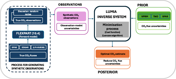
Figure 1. Diagram of the Observing System Simulation Experiment (OSSE) for determining the best atmospheric CO2 surface network across italy.
Download figure:
Standard image High-resolution image2.2. LUMIA inversion system
LUMIA is a Bayesian atmospheric inversion system that optimizes regional biosphere CO2 fluxes at a 0.25∘ resolution while prescribing anthropogenic, oceanic, and biomass burning emissions. The system minimizes a cost function by assimilating synthetic CO2 observations (section 2.6) over a one-year period in 2018, with a one-month spin-up at both ends of the optimization. To account for contributions not captured by regional fluxes, LUMIA estimates boundary conditions offline using either the two-step inversion method of Rödenbeck et al (2009), as applied by Monteil and Scholze (2021), or interpolated mixing ratios from global inversions such as CAMS (section 2.3). Regional transport is handled with precomputed observation 'footprints' from FLEXPART (Pisso et al 2019), while prior flux information is sourced from multiple datasets (section 2.4).
The system employs the Lanczos minimization algorithm (Lanczos 1950), which requires cost function gradients computed via forward and adjoint transport models. During optimization, Lanczos also derives the leading eigenvalues and eigenvectors of the posterior error covariance matrix, enabling posterior uncertainty reconstruction. The full prior and posterior covariance matrices account for variances and covariances, incorporating spatial and temporal error correlations. In LUMIA, the prior flux covariance follows a decaying exponential function. Further details on the system are provided in Monteil and Scholze (2021), and Gómez-Ortiz et al (2025).
2.3. FLEXPART atmospheric transport model
The LUMIA inversion system uses pre-computed observation footprints from the FLEXPART Lagrangian transport model (v10.4) (Pisso et al 2019). For 2018, FLEXPART was run backward in time (14 days) for each monitoring station shown in figure 1, releasing 10 000 particles continuously over each one-hour observation period. Footprints were computed by aggregating particle residence times in surface grid cells (below 100 m.a.g.l.). To estimate background CO2 mixing ratios, the final particle positions (latitude, longitude, time, and height) were used to interpolate CO2 fields from the Copernicus Atmosphere Monitoring Service (CAMS) global dataset (v18r3) (https://ads.atmosphere.copernicus.eu/datasets/cams-global-greenhouse-gas-inversion).
FLEXPART simulations were driven by meteorological fields from the ECMWF ERA5 reanalysis (https://www.ecmwf.int/en/forecasts/dataset/ecmwf-reanalysis-v5) at a 3 hourly temporal resolution and a 0.25∘ horizontal resolution. The regional domain extended from 33° to 73° N; 15° W to 35° E.
2.4. Prior and true fluxes
In OSSEs, a reference set of CO2 fluxes is considered the 'true' state and is used to generate synthetic observations that mimic real atmospheric measurements. These observations are produced by applying a transport model to the true fluxes and adding random noise to simulate measurement errors. This controlled setup allows for a direct evaluation of an inversion system by comparing recovered fluxes against the known true fluxes.
The true fluxes used in this study included biospheric, fossil fuel, fire, and ocean fluxes, sourced from different datasets. Biospheric fluxes (NEE) were taken from LPJ-GUESS (Wu et al 2023), which provides simulations at a 0.5∘ resolution and hourly timescales. Fossil fuel emissions were based on EDGAR v4.3.2 (Gerbig and Koch 2023), with MACC-TNO temporal variations (Denier van der Gon et al 2011) and COFFEE-based extrapolations (Steinbach et al 2011), both accessed via the ICOS Carbon Portal. Fire emissions were obtained from CAMS-GFAS https://ads.atmosphere.copernicus.eu/datasets/cams-global-fire-emissions-gfas, while ocean fluxes were from the Mercator Ocean biogeochemical analysis https://doi.org/10.48670/moi-00015, both produced for the CoCO2 project https://coco2-project.eu/.
Biospheric prior fluxes were represented by the VPRM model (Mahadevan et al 2008, Gerbig and Koch 2020), chosen for its differences from LPJ-GUESS, allowing for a clearer assessment of inversion adjustments. Prior fossil fuel emissions were taken from the TNO GHGco v4 dataset ( resolution), which was prescribed rather than optimized, given its well-characterized inventory-based nature. Similarly, fire and ocean fluxes were treated as fixed inputs, as they have a minimal impact on the net terrestrial CO2 flux in Europe. Spatio-temporal correlations for the prior uncertainties were defined to decay exponentially with a length of 500 km and 30 days for the biosphere fluxes. The length of the correlation used in this study is similar to what is used in other inversion systems in Europe (Thompson et al 2020, Monteil and Scholze 2021, Munassar et al 2023).

2.5. Synthetic observations
To generate the synthetic observations for our OSSEs experiments, we ran the regional transport model forward in time using the true assumed fluxes described in section 2.4. By utilizing these assumed true CO2 fluxes, we created a set of perfect ('truth') observations, which then were perturbed following the observational error statistics to generate the 'synthetic observations'. Such noise was added to reduce the impact of assuming a perfect atmospheric transport model.
For the control experiment (base network), the FLEXPART model was run using the same station configuration as described in the ObsPack dataset product of the actual (ICOS and non-ICOS) observations. Specifically, we used the same coordinates (latitude and longitude), surface altitude, and sampling height as described in the metadata of the ObsPack dataset (see supplementary, table S1). It is important to note that within the ObsPack product, observations are available at different sampling heights, so we selected only the highest sampling station.
For the Italian candidate stations, the model was run at the station locations described in supplementary information table S2. We assumed a sampling height of 100 m.a.g.l. for stations with low ground altitudes and 2 m.a.g.l. for mountain stations (e.g. if the station will be located at 1498 m.a.s.l., the sampling height will be 1500 m.a.s.l.). For all stations (both base network and new ones) with ground altitudes lower than 1000 m.a.s.l., we ran the model from 13:00 to 18:00 local time. For stations situated over mountainous terrain at altitudes higher than 1000 m.a.s.l., the model was run from 00:00 (midnight) to 05:00 local time. Assimilation of mountain observations at night is a common approach in atmospheric CO2 flux inversion, given that it favors the subsidence conditions characterizing free-tropospheric concentrations and avoids the need to re-solve daytime up-slope flows (Peters et al 2007, Lin et al 2017). Model-data mismatch errors are explained and shown in supplementary tables S1 and S2.
2.6. Base network, candidate stations and selection criteria
Our base atmospheric network (control experiment) relies on the European ObsPack dataset (ICOS RI et al 2023) for the year 2018 (supplementary information, table S1). This dataset includes both ICOS and non-ICOS stations. In 2018, four ICOS atmospheric stations were available in Italy: Lampedusa (LMP), Monte Cimone (CMN), Ispra (IPR), and Plateau Rosa (PRS). Potenza was incorporated in 2023; therefore, we added it to the base network to make the experiment more relevant to current conditions, as shown in figure 1 and supplementary information table S2.
For selecting candidate stations for the extended network, we considered 23 locations from Italy's existing monitoring infrastructure, as well as potential future stations. From the current infrastructure, we selected 15 ICOS ecosystem stations, 5 non-ICOS atmospheric stations, and 3 potential future stations (Chieti (CHI), Monte Venda (VND), and Col Margherita (MRG)) as listed in supplementary information table S2.
Our first OSSE experiment (excluding the control run) involved running the LUMIA inversion system 23 times, defined as experiment S01A. For each run in experiment S01A, we added one station at a time from the candidate list (shown in the supplementary information, table S3) to our base European network. This approach allowed us to evaluate which of the 23 selected sites contributed the most to improving the reconstruction of the true flux values and reducing prior flux uncertainties. Given the lack of stations in the southern part of Italy, our selection criteria mainly rely on selecting the sites that bring more information to that area of the country through the evaluation of different statistical metrics explained in section 2.7.
In total, we conducted five experiments, each building on the results of the previous one. In the second experiment (S01B), we repeated the process used in S01A with the remaining 22 stations. We followed the same approach in the third experiment (S01C), where the inversion was run with the remaining 21 candidate stations, and in the fourth experiment (S01D), with 20 candidate stations. This process can be seen as an incremental optimization scheme, where each station that provides the best true flux reconstruction and the greatest uncertainty reduction is added to the network and removed from the candidate list. The fifth experiment, defined as S01, was conducted by running the inversion with all 23 sites together.
2.7. Network design evaluation metrics
The performance of each hypothetical station was evaluated by assessing how well the LUMIA system reconstructs the 'known' true fluxes, defined here as those generated by the LPJ-GUESS model. To measure this performance, we computed several statistical metrics, including mean bias (MB), root mean square error (RMSE), and Pearson's correlation coefficient. Biases were calculated as the differences between the true fluxes and the control. The same approach was applied to the prior and posterior fluxes (e.g. for each scenario of the extended network). These metrics were computed for weekly resampled flux data across various regions (Northern, Central, and Southern Italy) as shown in figure 2.

Figure 2. European domain of the LUMIA inverse system, showing the European ObsPack stations (base network) from our study, with the hypothetical atmospheric extended network for Italy highlighted in the red box.
Download figure:
Standard image High-resolution imageTo assess the improvement in the relative reduction of prior biases, we calculated the percentage bias reduction as:

Similarly, the percentage uncertainty reduction was computed as:

Where prior and posterior represent the standard deviation (SD) of the prior and posterior flux uncertainties, respectively. The percentage of uncertainty reduction accounts for both variances and covariances. Specifically, both the prior and posterior covariance matrices were computed as the product of the emission uncertainties and the correlation matrix, as explained in section 2.4.
3. Results
3.1. Reconstructing the true state with the extended Italian atmospheric network
Figure 3(a) shows that the current base ICOS network in Italy provides a good constraint on carbon fluxes throughout the country. We observe that prior biases are reduced from −1.18 (RMSE: 2.36) to −0.21 (RMSE: 0.67) TgC week−1, corresponding to an 82.5% reduction in bias. With the addition of the CHI station to the network (obtained from experiment S01A), the bias in the seasonal cycle for Italy is further reduced to −0.10 (RMSE: 0.59) TgC week−1, representing a 92% reduction-an additional 10% improvement over the current network. In terms of flux uncertainty reduction, the CHI site contributes to an overall 29% decrease in uncertainty across Italy (figure 4(a)). This impact is primarily driven by a combination of the spatial extent of its footprint (supplementary information, figure S3) and correlation effects, which are further discussed in section 3.2. The representativeness of the CHI site (footprint) extends from central-eastern Italy, between the Apennine Mountains and the Adriatic coastline, toward the north, improving constraints beyond the influence of the existing northern sites.
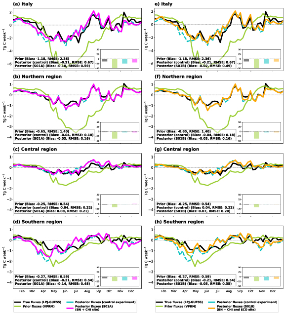
Figure 3. Right panels show the seasonal cycle of weekly CO2 fluxes for 2018 (experiment S01A) aggregated across (a) all of Italy, and divided into three sub-regions: (b) Northern, (c) Central, and (d) Southern areas of the country. Left panels (e)–(h) show the same as the right panels but for experiment S01B. Inset bar plots in the lower right corner of each panel represent the annual CO2 fluxes aggregated for 2018 (Units: TgC yr−1). Uncertainties are not included in this figure to better illustrate the magnitude of the annual carbon fluxes.
Download figure:
Standard image High-resolution image
Figure 4. Box plots of bias, root mean squared error (RMSE), and Pearson correlation coefficient (R) for the OSSE S01A (left panels) and S01B (right panels) experiments. Results for the southern region are highlighted with yellow-filled boxes. Sites highlighted in blue (first-row panels) correspond to those providing the highest uncertainty reduction by region. Red-highlighted sites (second-row panels) indicate those with the highest bias reduction, which are also associated with the lowest RMSE (third row) and highest correlation (fourth row).
Download figure:
Standard image High-resolution imageA significant improvement in biases is also observed in the northern part of Italy (figure 3(b)) (considering only the base network). The prior biases and RMSEs in Northern Italy decrease from −0.65 (RMSE: 1.40) to −0.04 (RMSE: 0.18) TgC week−1 in the control experiment, which represents a bias reduction of 94% and 87% in RMSE. The addition of the CHI station to the network does not have much influence in the northern region, as the biases remain almost the same. These results were expected in some way, since the current network is concentrated mostly in the northern part of the country, as shown in figure 5(a). In this region, the IT-MBO site contributes the most to flux uncertainty reduction, as shown in figure 4(b). Footprints in this area extends from Monte Bondone, a mountain in the northeastern Italian Alps, toward the northwest, reaching Monte Cimone (supplementary information, figure S3).

Figure 5. Fractional uncertainty reduction (%) of the posterior flux uncertainties relative to the prior flux uncertainties.
Download figure:
Standard image High-resolution imageIn central Italy (figure 3(b)), we see that the current network reduces the bias from −0.25 to 0.04 TgC week−1. Even though the posterior biases are closer to zero and indicate a substantial reduction in bias error, we also see a slight overcorrection that shifted the bias to a small positive value. CHI site, also has a strong influence in the central region, where the uncertainty flux reduction reach 29%.
In Southern Italy (figure 3(c)), the current base network reduces prior biases by only 23%, with biases decreasing from −0.27 (RMSE: 0.59) to −0.21 (RMSE: 0.54) TgC week−1. Adding CHI to the network further decreases prior biases from −0.21 (RMSE: 0.54) to −0.14 (RMSE: 0.48), representing a 48% reduction and an additional 25% improvement over the existing network. In this southern region, the CHI site provides the strongest constraint on fluxes compared with other sites, with uncertainty reduction reaching 24% versus 21.6%–22.8% (figure 4(a)).
Given the above results, our selection criteria focused primarily on improving the southern region of Italy, where only the Potenza (POT) station is located. We further explored the potential of the existing Italian network by performing the inversion again with the remaining 22 stations (while keeping the CHI site fixed in the network; experiment S01B), to then select the combination that provided the best constraint on fluxes in the southern region.
Our analysis of experiment S01B identified Lecce (ECO), located in the heel of the Italian Peninsula (as shown in figure 3(h), as the station providing the strongest additional constraint on southern fluxes, not only because it reduces the prior biases from −0.27 to −0.05 TgC week−1, an 82% reduction relative to control experiment (23%), but also because it achieves the largest RMSE reduction (0.35) and the highest correlation (R = 0.72) among all 22 sites (figures 4(g) and (h)). Adding CHI and ECO together translates to a 34% overall improvement, which is an additional 59% better than the existing network.
Another site, apart from the combination of CHI and ECO, that also provides a significant prior bias reduction is CGR (bias = −0.04 TgC week−1). However, this station has a lower RMSE reduction (0.40 TgC week−1) and correlation (R = 0.66) compared to the CHI-ECO sites (Supplementary table S7). CHI-IT-CP2 also leads to a significant bias reduction (−0.07 TgC week−1), but its impact on bias reduction in the southern region is limited to 74%, approximately 8% less than the reduction achieved when the ECO station is selected in combination with CHI.
Adding a third station to the new network, while keeping CHI and ECO fixed, as shown in table S8 (supplementary information), results in only marginal improvements in reducing prior biases in southern Italy. Most station combinations produce posterior biases between −0.01 and −0.13 TgC week−1. We selected IT-SAS as a potential third site, despite its slightly higher bias (−0.10 TgC week−1) compared to other options, because it provides the highest correlation (R = 0.78) and the lowest RMSE (0.31 TgC week−1) among the available sites. While IT-SAS shows a slightly higher bias, its lower RMSE and stronger correlation make it a preferable choice. A lower RMSE indicates smaller and more consistent errors, while a higher correlation suggests better agreement with flux variations over time. This trade-off is relevant since biases can often be corrected more easily than high RMSE, which reflects greater variability. Selecting a site with more stable and predictable error characteristics ultimately strengthens the network's ability to constrain regional fluxes. Other potential sites in the southern region, such as IT-COL and IT-CP2, offer slightly better biases (−0.01 and 0.03 TgC week−1, respectively) but result in a smaller RMSE reduction (0.34) and lower correlation (R = 0.74) compared to the CHI-ECO-IT-SAS combination.
A fourth combination suggests that adding IT-PCM to a network that already includes CHI, ECO, and IT-SAS (supplementary information table S9) further improves the correlation (R = 0.82), RMSE (0.28 TgC week−1), and bias (−0.02 TgC week−1). Adding IT-SAS and IT-PCM as the third and fourth sites results in a 93% improvement relative to the current base network. This represents an additional 12% improvement beyond the 82% gain already achieved with CHI and ECO alone.
We also evaluated the impact of incorporating all 23 hypothetical stations (as shown in figure 5(f) and supplementary information figure S4) into Italy's atmospheric network and found that the bias reduction (0.74%) is similar in magnitude to that achieved when CHI-ECO sites are added (82%). This suggests that simply increasing the number of sites in the network does not necessarily improve the statistical metrics (bias, RMSE, or R) of the posterior fluxes. These findings were, to some extent, expected, given that the prior error correlation length used in the inversion was set to 500 km. In the discussion section (4), we further demonstrate that even reducing the correlation length to 100 km remains insufficient to fully take advantage of all 23 sites in the network. Since atmospheric CO2 observations are sparse in both Europe and Italy, a prior error correlation length of 500 km is still reasonable, as observations are often far apart. Increasing the number of sites in the atmospheric network would require further reducing the correlation length to fully capture the influence of each observation on estimated fluxes at nearby locations.
3.2. Relative uncertainty reduction at grid-cell level scale
We saw in the previous section that the CHI station (figure 4(a)) was one of the sites that provides the best constraint on fluxes across Italy (uncertainty reduction of 29%), central (uncertainty reduction of 28%), and southern region of Italy (uncertainty reduction 24%), with an exception the northern region, where Monte Bondone (IT-MBO) contributes to a 33% reduction in uncertainty when aggregated over that area.
At grid-cell scale, as shown in figure 5, we see around the CHI station, uncertainties reduction is approximately 30%, and gradually decreases to 28%–26% near the Apennines (Maiella ridge, 2700 m), which extends from north to south along the Italian peninsula. These results are somewhat expected, as the sensitivity of the CHI site decreases in this area (supplementary information, figure S3). This underscores the importance of the uncertainty correlation length within the prior error covariance matrix, which enables more extensive constraints on fluxes beyond the immediate vicinity of the station.
Figures 5(c)–(e) show that adding other stations such as ECO, IT-SAS, and IT-PCM to the Italy-based network increases the uncertainty reduction in southern Italy, although the impact is less significant compared to considering the CHI station alone. When all 23 sites are added, the uncertainties in the southern region of Italy improve only slightly. However, additional stations in the northern region lead to a substantial reduction in uncertainty, reaching up to 40% around the Monte Bondone (IT-MBO; figure 2) station, with values gradually decreasing to 37% in its vicinity.
4. Discussion
Expanding national-scale atmospheric CO2 monitoring networks is crucial for improving top–down estimates of CO2 surface fluxes. In this study, we assess the potential benefits of adding 23 additional existing sites to Italy's ICOS atmospheric network as a case study within Europe, given the country's lack of GHG monitoring stations in the south. One of our main findings suggests that CHI and ECO are the most suitable locations for expanding Italy's current ICOS network, which currently includes Plateau Rosa, Ispra, Monte Cimone, Potenza, and Lampedusa. The addition of these two sites significantly enhances flux constraints in southern Italy, reducing weekly seasonal biases by approximately 82% in an OSSE context. In comparison, the existing network reduces prior biases by only 20%, underscoring the value of expanding the network towards the south.
Unlike other continental-scale network design studies, which focus primarily on selecting optimal sites based on uncertainty reduction metrics (e.g. Ziehn et al 2014, Nickless et al 2015, Kaminski and Rayner 2017), our study is the first to assess optimal network design by evaluating both the reconstruction of true fluxes and the quantification of uncertainty reduction. As far as we know, no previous network design studies have focused specifically on Italy, and the results presented here provide a first step toward filling this gap, offering a targeted assessment for improving the country's CO2 observation network. This study could serve as a baseline for future network design efforts in Italy, providing a foundation for guiding the placement of additional atmospheric stations. Since our study is the first network design study focusing specifically on Italy, a direct comparison with other results is not possible at this stage.
Regarding the OSSE configuration, it is important to note that the selection of CHI and ECO is closely linked to the LUMIA inversion setup, which uses the FLEXPART model at 0.25∘ resolution, along with the assumptions made for each component of the inversion. Therefore, our study neglects transport errors, and the improvements in terms of bias and uncertainty reduction could differ if other models were used (e.g. an Eulerian instead of a Lagrangian model). Differences in transport representation, including boundary layer mixing, advection, and model resolution, can significantly influence the sensitivity of the inversion to observational constraints. Besides, the spatial correlation structure of prior flux uncertainties may interact differently with transport errors across models, further impacting the optimal network configuration. As such, further research using alternative transport models would be valuable to assess the robustness of our site selection results.
Although this study cannot be directly compared with other network design efforts in Italy (as, to our knowledge, none exist), the selection of a 500 km spatial correlation length for the prior error covariance matrix is consistent with previous inversion studies over Europe (e.g. Thompson et al 2020, Monteil and Scholze 2021, Munassar et al 2023). Given the sparse atmospheric network in Italy, our results confirm that a 500 km correlation length remains a reasonable assumption, as evidenced by the improvement in posterior flux estimates in the control experiment.
The choice of prior error covariance correlation length is a key factor in inverse modeling, as it not only defines how uncertainties in surface fluxes are spatially correlated but also determines how information from individual observations influences flux estimates at nearby locations. In our OSSEs, we found that reducing the prior error covariance correlation length to 100 km was insufficient to fully exploit the addition of 23 new sites to the Italian network (figure S4, supplementary information). These findings suggest that to maximize the benefit of the expanded network, OSSEs should be conducted at a high-resolution scale (e.g. 10 km), where a shorter prior error covariance length can better capture local flux variations. This enables observations from closely located sites to have a stronger influence on nearby flux estimates, potentially improving corrections-provided that the chosen correlation length aligns with the spatial characteristics of real flux variability.

We note that this research aims to explore, under realistic scenarios, which additional stations in Italy would provide the most useful information to the system if implemented, taking into account the existing European ICOS and non-ICOS stations. Given that this study specifically targets biosphere CO2 fluxes, the results may differ for anthropogenic CO2 emissions or other species, such as CH4, which involve distinct spatial distributions and emission processes. Consequently, an optimal network configuration may vary depending on the focus on different sources or gases. Additionally, although this study did not directly assess this, we believe that adding another station in the Po Valley could be particularly valuable due to the region's intense agricultural and industrial activity. The Po Valley is currently constrained by only one mountain site (Monte Cimone), which may limit the ability to accurately capture emissions in this highly active area. Nonetheless, our findings suggest that further research funding should prioritize the CHI and ECO stations, as these locations have demonstrated the most significant value in enhancing the accuracy and precision of flux estimates in southern Italy.
5. Conclusion
We conducted a series of OSSEs using the LUMIA regional inverse system to assess the impact of expanding atmospheric CO2 monitoring networks, using Italy as a case study. Expanding the Italian network significantly enhances flux accuracy and precision, particularly in southern Italy, where only Potenza currently serves as an ICOS atmospheric station. The inclusion of the CHI station alone reduces flux uncertainties by 24% and prior biases by approximately 48%, while adding both CHI and ECO further improves accuracy, reducing biases by 82%. However, adding more than these two stations results in only marginal improvements in flux precision, indicating that a targeted selection approach is more effective than widespread network expansion.
While these findings indicate that adding two stations to the ICOS network would be particularly beneficial for constraining fluxes in southern Italy, there are limitations to our approach. Notably, the study relies on a perfect transport and perfect background assumption, which simplifies real-world complexities and may not fully capture uncertainties in transport and boundary conditions. Despite this, our results provide insights that could guide network design for carbon monitoring in underrepresented regions, especially where achieving optimal flux constraints at a national scale is essential. We demonstrated our network design approach for the example of Italy, but the methodology can be transferred to any other national monitoring network.
Acknowledgments
This study acknowledges support from the EU projects AVENGERS (Grant Agreement (GA): 101081322), and from three Swedish strategic research areas: ModElling the Regional and Global Earth system (MERGE), the e-science collaboration (eSSENCE), and Biodiversity and Ecosystems in a Changing Climate (BECC). Computational resources were provided by the National Academic Infrastructure for Supercomputing in Sweden (NAISS), the Swedish National Infrastructure for Computing (SNIC) at LUNARC, and NSC partially funded by the Swedish Research Council through Grant Agreements Nos. 2022-06725 and 2018-05973, and the Royal Physiographic Society of Lund through Endowments for the Natural Sciences, Medicine and Technology—Geoscience.
Data availability statement
The dataset associated with this study, which includes statistical metrics of the OSSEs, is available at https://doi.org/10.5281/zenodo.14887163.