

Abstract
Extratropical cyclones play a crucial role in balancing the global momentum, energy, and moisture, and also, they shape the extreme weather events over the extra-tropics. As the strongest category of the extratropical cyclones, the explosive extratropical cyclones (EECs) frequently induce severe disasters through their strong surface winds. During the entire lifespan of an EEC, there is a maximum value of its surface wind (i.e. the maximum surface wind; MSW), which processes the greatest destructive power. After nearly a century of research on the EECs, key features about their MSWs still remain vague. In this study, we systematically investigate the EECs' MSWs over the North Atlantic storm track (NAST) based on the ERA-Interim reanalysis. It is found that, the average intensity of EECs' MSWs shows a significant increasing trend of ∼0.3 m s−1 per 10a. More importantly, for the last 20 years, even larger increasing rates of 1.5 m s−1 and 3.5 m s−1 per 10a are found in the average and maximum intensities of the EECs' MSWs, respectively, implying the EECs' risks increase notably for the NAST. We further clarify the physical mechanisms governing the production of EECs' MSWs, and then establish a mechanism-based statistical model, which has the potential to predict the MSWs' annual average intensity. In summary, our study fills a knowledge gap for the EECs' MSWs, which would have broad implication of the economics and society.
Export citation and abstract BibTeX RIS

Original content from this work may be used under the terms of the Creative Commons Attribution 4.0 license. Any further distribution of this work must maintain attribution to the author(s) and the title of the work, journal citation and DOI.
1. Introduction
In cold seasons, winter storms are the most dangerous weather systems due to their huge societal and economic impacts (Hewson and Neu 2015). For instance, on 27 January 2021, the strong winds (peaking at near 26.8 m s−1; www.ijpr.org/weather/2021-01-27/tens-of-thousands-without-power-as-winter-storm-pummels-northern-california) associated with the winter storm 'Orlena' had downed trees and power lines throughout northern California, resulting in serious power outages across the region, with over 390 000 utility customers lost power (https://blog.norwall.com/winter-weather/winter- storm-orlena-2021-noreaster-pummels-northeast/). In early December 2021, winter storm 'Barra' brought deadly strong winds to Western Europe, with a wind speed of up to 97.5 mph observed at the Fastnet Lighthouse, Ireland. Strong winds associated with the storm had left at least 59 000 people without power in Ireland, resulting in significant social impacts (https://news.sky.com/story/storm-barra-rain-snow-and-80mph-winds-forecast-to-batter-uk-amid-danger-to-life-weather-warning-12488486).
In meteorology, the winter storms called the explosive extratropical cyclones (EECs) are defined as the extratropical cyclones that deepen in their central pressure by at least 24 hPa (relative to the equivalent latitude of 60°) in one day (Sanders and Gyakum 1980). Generally, the radii of the EECs are ranging from 500 km to 2000 km during their mature stage (Jiang et al 2021a). The EECs' rapid intensification causes strong winds surrounding the cyclones' centers. Although most of the EECs-associated strong winds appear over ocean (Zhang et al 2017, Jiang et al 2021a, 2021b), a few of them occur over land and coastal regions, which poses a great threat to these areas (Browning 2004, Knox et al 2011, Fu et al 2014, Booth et al 2015, Brâncuş et al 2019, Jiang et al 2021a, 2021b). Of the EEC-associated strong surface winds, there is a maximum value during the cyclone's whole lifespan. Jiang et al (2021a) define it as the maximum surface wind (MSW) of the EEC, which has the greatest destructive power among all strong winds associated with the EEC. Although the EECs have been investigated for almost a century (e.g. Sanders and Gyakum 1980, Sanders 1987, Davis et al 1996, Yoshida and Asuma 2004, Kuwano-Yoshida and Asuma 2008, Hirata et al 2015, Fu et al 2018, 2020), there still remains a knowledge gap about their MSWs. Key features including the MSWs' horizontal distribution, formation mechanisms, and long-term trend, all remain vague.
According to previous studies (Allen et al 2010, Fu et al 2020), the North Atlantic storm track (NAST) (Hoskins and Valdes 1990) is one of the most active areas for the EECs (figure 1(a)). In this study, we use the 40 year tracking statistics from Jiang et al (2021a) (i.e. the union of all tracks in figure 2) to estimate the range of the NAST. According to the American Meteorological Society (https://glossary.ametsoc.org/wiki/Storm_track), the storm track is a region in which the synoptic eddy activity is statistically and locally most prevalent and intense. It roughly corresponds to the cyclones' trajectories. After analyzing the strong winds associated with 961 EECs in this area, Jiang et al (2021a) found that, the EECs over the NAST had a mean MSW ranging from 27.3 m s−1 to 30.4 m s−1, which was higher than the threshold of 26 m s−1 for a high-wind event defined by the US National Weather Service (Lacke et al 2007, Knox et al 2011, Booth et al 2015). Strong winds of this intensity can induce huge ocean waves with a wave-height of ∼10 m, which is fatal to most ships in the ocean. Furthermore, strong winds associated with the EECs can induce upwelling up to a depth of 6000 m inside the ocean (Kuwano-Yoshida et al 2017), which result in a notable cooling in upper oceans.
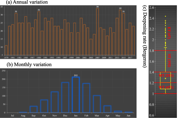
Figure 1. Annual (a) and monthly (b) variations of all EECs over the target region, where white values mark the cyclones' numbers. Panel (c) is the box whisker diagram of cyclones' deepening rates (Bergeron). The yellow box indicates the 25th (Q1) to 75th (Q3) percentiles, the small yellow cross represents the mean value, and the yellow line indicates the median value; the whiskers indicate the range of [Q1 – 1.5 × (Q3 – Q1)] (or the minimum of the data) and [Q3 + 1.5 × (Q3 – Q1)] (or the maximum of the data); the small yellow hollow circles are values beyond the upper whisker. The red dashed lines outline the deepening rates used to divide all the cyclones in to the extreme type (ET), strong type (ST), moderate type (MT) and weak type (WT). The red values within the parentheses are the cyclones' numbers of the corresponding types.
Download figure:
Standard image High-resolution image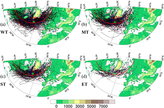
Figure 2. Panels (a)–(d) show the tracks (black solid lines with small black open boxes representing their formation location and small black closed circles indicating their dissipation locations) of the WT, MT, ST and ET, respectively. The small closed blue circle marks the location of the cyclone's center when its MSW appeared, and the small closed red circle marks the location of the MSW. The thick red line shows the clustering track of the corresponding types of cyclones and the green open box shows the averaged location of all MSWs.
Download figure:
Standard image High-resolution imageAs discussed above, to further the understanding of the EECs-associated disastrous weathers deserves a profound study on their MSWs. In order to fill the current knowledge gap of the EECs' MSWs, the first scientific purpose is to explore the main statistical features of the MSWs over the NAST, and to determine the formation mechanisms for them. Moreover, in recent cold seasons, many news reports are related to the EECs over the NAST, which might make us feel that the EECs' impacts are increasing. Whether true or not, this needs a quantitative study to clarify the real situation. Therefore, the second scientific purpose of this study is to show the variational trends of the EECs' MSWs over the NAST. After solving the two scientific questions, we attempt to develop useful indices for estimating the EECs' MSWs.
2. Data and methods
Jiang et al (2021a) conducted a 40 year (1979–2018) statistical study on the EECs in the Northern Hemisphere based on the 6 hourly 0.75° × 0.75° ERA-Interim reanalysis data (https://doi.org/10.5065/D6CR5RD9) from the European Centre for Medium-Range Weather Forecasts. As evaluated by previous studies (Ramon et al 2019, Fan et al 2021), the ERA-Interim reanalysis shows a credible skill for representing the surface winds. Therefore, it have been widely used for analyzing the strong winds associated with the extratropical cyclones (Martínez-Alvarado et al 2012, Hart et al 2017, Hirata 2021). Nevertheless, ERA-Interim is mainly capable of revealing the synoptic-scale winds associated with extratropical cyclones (Hart et al 2017). Generally, the multi-year reanalysis datasets (including ERA-Interim) cannot resolve the mesoscale flows (Martínez-Alvarado et al 2012, 2013, Clark and Gray 2018), such as the sting jets (Browning 2004, Clark et al 2005), which are even challenging to be accurately observed (Bourassa et al 2019). Jiang et al (2021a) used the eight-section-slope detecting method to detect the cyclone structures (Jiang et al 2020); and they used the moving distance and similarity (i.e. field correlation) to track the cyclone structures. After manual verifications (which had removed almost all errors that could not be solved by the objective detecting/tracking algorithms themselves), Jiang et al (2021a) determined a total of 961 EECs over the NAST. We used the method proposed by Yoshida and Asuma (2004) to calculate the deepening rate of an EEC:
where t is time (h), p is the cyclone's central sea level pressure (hPa), and φ is the latitude of the cyclone's center. In addition to the EAR-Interim dataset, the monthly, 0.25° × 0.25° surface skin temperature (i.e. surface temperature) and vertical velocity from the ERA5 dataset (Hersbach et al 2020) were used to analyze the variations of the temperature and vertical motions (VMOs).
Similar to Messmer and Simmonds (2021), Jiang et al (2021a) used the radius of 2000 km to determine the strong surface winds associated with an EEC. Of all the strong surface winds associated with an EEC during its whole lifespan, the largest value was defined as its MSW. The time when an EEC's MSW appeared was defined as the maximum surface-wind time. The time when an EEC reached the largest deepening rate during its whole life span was defined as the maximum deepening time. The distances between the locations where the MSWs appeared and the corresponding EECs' centers (DMCs) were used to represent the MSWs' radial distribution.
To understand the mechanisms related to the distribution of EECs' MSWs, we used two factors: (i) the moving speed of an EEC at t was represented by the moving speed of its center from t − 1 to t (the wind associated with an EEC was the superposition of the EEC-relative wind and the cyclone's moving speed). (ii) The baroclinic energy conversion (BEC) was calculated by BEC = −αω, where α is the specific volume, and ω is the vertical velocity in the pressure coordinate. For EECs, which are characterized by strong baroclinity, a positive BEC denotes the energy is transferred from the available potential energy to the kinetic energy (KE; KE = (u2 + v2)/2, where u and v are zonal and meridional wind, respectively) (Lorenz 1955, Murakami 2011, Fu et al 2016), which directly enhances the wind speed. After calculating 224 Northwest Pacific wintertime EECs, Black and Pezza (2013) summarized that, the BEC was the only dominant term accounting for the enhancement in EECs' wind speed. Sampe and Xie (2007) also regarded baroclinity as a key mechanism for explaining the high winds over ocean. In addition to BEC, Sampe and Xie (2007) found another important mechanism for producing the high sea winds—the boundary layer momentum mixing. They proposed that, near a sea surface temperature front, the surface air temperature was in disequilibrium with the sea surface temperature due to the larger-scale atmospheric adjustment. This resulted in an unstable atmosphere on the warmer flank of the sea surface temperature front with strong turbulent mixing that brought down stronger winds from aloft, enhancing the surface wind.
3. Statistical features
3.1. General features
The mean, least and largest annual occurrence frequencies of the EECs over the NAST were 24, 11 and 34, respectively (figure 1(a)), with no significant linear trend detected in the EECs' annual occurrence frequency. More EECs tended to occur in winter (figure 1(b)), particularly for January, with ∼5.3 EECs appeared in January on average. In contrast, EECs showed the least occurrence frequency in summer, with no EECs in July. Compared with previous studies (Lim and Simmonds 2002, Allen et al 2010, Fu et al 2020), the annual occurrence frequency of the EECs are different, as the datasets and standards used for determining EECs are different. However, most of the previous studies also have confirmed that (i) the EECs show a much larger occurrence frequency in winter than that in summer; and (i) there is no significant linear trend in their annual frequency over the Northern Hemisphere. The EECs' deepening rates were mainly smaller than 3.0 Bergeron (figure 1(c)): (i) ∼50% of them was smaller than 1.2 Bergeron, which were defined as the weak type (WT); (ii) ∼25% of the EECs had a deepening rate of 1.2–1.4 Bergeron, which were defined as the moderate type (MT); (iii) the remaining 25% of the EECs were further classified by using 1.8 Bergeron into the strong type (ST; ∼20%) and the extreme type (ET; ∼5%).
The EECs-associated MSWs (small closed red circles in figure 2) covered ⩾50% of the range of the North Atlantic Ocean. The highest frequency of the MSWs appeared around the region of 55 °N–65 °N, 40 °W–50 °W, and the lowest frequency appeared around the region of 25 °N–35 °N, 30 °W–0 °W. This distribution was consistent with the EEC's northeastward moving tracks. As shown in figure 2, much more MSWs appeared over the Ocean than that occurred over land. This is mainly because (i) much more EECs tended to enter their explosive developing stage over the ocean due to the much stronger latent heat release (Fu et al 2014, 2018), and (ii) the friction over land was much great than that over the ocean. As the intensity grew, EECs' influencing range shrank in size, whereas, the proportion of the MSWs that appeared over Ocean increased.
3.2. Octant distribution
We used the octants 1–8 (O1–O8; as figure 3(a) shows, they increased by an interval of 45° counterclockwise) to clarify the distribution of MSWs. Overall, for all EECs, O2 and O1 occupied the largest (∼18.4%) and the second (∼15.9%) largest proportions of MSWs (figure 3(a)), and their respective maximum/mean MSWs were the second strongest (46.0/30.2 m s−1) and the strongest (46.7/30.7 m s−1). These indicate that, O1 and O2 were the most dangerous octants for the EECs. In contrast, O4 showed the smallest proportion of MSWs, whereas, the smallest maximum/mean MSWs appeared within O5 (37.5 m s−1) and O7 (26.8 m s−1), respectively. For the WT, MT and ST, O2 also possessed the largest proportion of MSWs (figures 3(b)–(d)), whereas, for the ET, O1 was the largest (figure 3(e)). Moreover, for all the four types of EECs, their O4 had the smallest proportion of MSWs (figures 3(b)–(e)).

Figure 3. Panel (a) shows the proportion of occurrence of the MSWs in octants 1–8 (O1–O8), the corresponding averaged MSWs (m s−1) and the largest MSW (m s−1) within each octant for all EECs, where the green shading shows the octant with the largest proportion of MSWs. Panels (b)–(e) are the same as (a) but for the WT, MT, ST, and ET, respectively. Panel (f) illustrates the averaged moving speed of the EECs (m s−1) in the x- and y-directions, and their composite, respectively. Panel (g) shows the boxplots of the distance between the locations of the MSW and the EEC's center (DMC; km) for different types of EECs. The boxes indicate the 25th (Q1) to 75th (Q3) percentiles, the small crosses represent the mean values, and the yellow lines indicate the median values; the whiskers indicate the range of [Q1 – 1.5 × (Q3 – Q1)] (or the minimum of the data) and [Q3 + 1.5 × (Q3 – Q1)] (or the maximum of the data), and the outliers are removed.
Download figure:
Standard image High-resolution imageFrom WT to ET, as the EECs' intensity grew (figures 3(b)–(e)): (i) the accumulated proportion of O1 and O2 (i.e. cyclones' northeastern section) increased (from ∼31.6% to ∼44.6%); (ii) the proportion of O4, which occupied the least proportion of MSWs, decreased consistently (from ∼8.1% to ∼2.1%); (iii) the value of the largest/smallest mean MSW increased (from 30/25.8 m s−1 to 35.8/27.7 m s−1); and (iv) the ratio of cyclone's moving speed in the x-direction to that in the y-direction (figure 3(f)) increased. All these mean that, the EECs' MSWs showed a notable intensity-dependent feature, and as the intensity grew, O1 and O2 became more dangerous.
Most of the MSWs (>75%) appeared within 300–800 km from the EECs' centers (figure 3(g)). On average, for WT, its octant-averaged DMC was ranging from ∼400 km (O5) to ∼730 km (O7); for MT, the counterpart was from ∼400 km (O5) to ∼680 km (O2); for ST, the counterpart was from ∼400 km (O5) to ∼620 km (O7); and for ET, the counterpart was from ∼300 km (O7) to ∼730 km (O8). Overall, for the WT, MT and ST, O5 possessed the least DMC, and as EECs' intensity grew, the MSWs became closer to the cyclones' centers, whereas, the ET showed a different feature.
4. Mechanisms governing the formation of MSWs
4.1. Baroclinic energy conversion (BEC)
According to the KE budget equation (Lorenz 1955, Murakami 2011, Black and Pezza 2013), the horizontal/vertical advection and the BEC all acted as crucial factors for the KE's variation. Because the MSW is the largest surface wind within a radius of 2000 km from the cyclone's center during its whole life span, the MSW cannot be caused by the horizontal advection (because there are no inverse gradient advection). In addition, since the regions surrounding the EECs' centers were mainly dominated by notable ascending motions (figure 16 of Jiang et al (2021a)), the downward momentum transport was weak, and could not be a key reason to produce the EECs' MSWs either.
As mentioned above, the EECs' MSWs were not caused by transport (i.e., the horizontal/vertical advection), and thus, the BEC might play a crucial role. Because the EECs' MSWs tended to appear after the cyclones gained their maximum deepening rates (Jiang et al 2021a), two typical stages (i.e. the maximum deepening time and the maximum surface-wind time) were used to analyze the BEC's contribution. From figure 4, it is clear that, for both the maximum deepening time and the maximum surface-wind time, strong positive BEC appeared within O1 and O2 (i.e., the EECs' northeastern section). For the arithmetic mean of these two stages, O1 and O2 ranked first and second in terms of the intensity of BEC for all types of EECs. This was consistent with the fact that the largest proportion of MSWs appeared within O1 and O2 (section 3.2). Moreover, as EECs' intensity grew, within O1 and O2, the BEC enhanced notably in intensity, and the region with strong positive BEC enlarged remarkably in area. These explained the fact that as the EECs' intensity grew, (i) more MSWs appeared within O1–O2 (from ∼31.6% to ∼44.6%), and (ii) the mean speed of MSWs in these two octants enhanced (from ∼29.4 m s−1 to ∼35.5 m s−1). Therefore, we concluded that, the strong BEC that transferred the available potential energy to KE was a key reason for producing the EECs' MSWs.

Figure 4. Panels (a)–(d) show the composite (based on the Lagrange viewpoint) vertical averaged (from surface to 500 hPa) baroclinic energy conversion (BEC) (shading; W kg−1) of the WT, MT, ST and ET, respectively, when the cyclones gained their maximum deepening rates. The white dot shows EECs' centers, and the white radius is 1350 km. MDT = maximum deepening-rate time. Panels (e)–(h) are the same as (a)–(d) but for the maximum surface-wind time (MST).
Download figure:
Standard image High-resolution image4.2. Superposition effects
The EECs' MSWs were the results of the superposition of the EECs' moving with the cyclone relative wind. On average, the EECs' moving speed was arranging from 6.3 m s−1 to 8.1 m s−1 (figure 3(f)), implying that it played an indispensable role in generating the EECs' MSWs. After superposition, compared the MSW's intensity with that of the EEC relative wind, there were mainly two situations: (i) the MSW was larger (i.e. the enhancing superposition); and (ii) the MSW was smaller (the abating superposition).
For all EECs, their MSWs and the cyclone-relative winds rotated counterclockwise from O1 to O8, which were consistent with the cyclonic circulation of the EECs. Within O6–O8, for all types of EECs, their MSWs were 5% (figure 5(ζ))–100% (figure 5( )) larger than the corresponding cyclone relative winds. This means that, the enhancing superposition appeared within these octants. In contrast, within O1–O5, for all types of EECs, their MSWs were 0% (figure 5(β))–17% (figure 5(z)) smaller than the corresponding cyclone relative winds, implying that an abating superposition occurred. This confirmed that, the MSWs within O1 and O2 were mainly produced by the BEC, as the superposition was mainly detrimental.
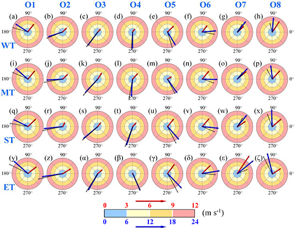
Figure 5. Panel (a) shows the averaged moving speed (red vector; m s−1; referring to the red numbers over the color bar) of the WT, associated with which the MSWs appeared within octant 1 (O1). Averaged MSWs of these cyclones are shown by the blue vector (m s−1; referring to the blue numbers below the color bar). Black vectors are the EEC relative winds calculated by averaged MSWs minus the averaged moving speed (m s−1; referring to the blue numbers below the color bar). Panels (b)–(h) are the same as (a) but for O2–O8, respectively. Panels (i)–(p) are the same as (a)–(h), but for the MT. Panels (q)–(x) are the same as (a)–(h), but for the ST. Panels (y)–(ζ) are the same as (a)–(h), but for the ET. Concentric circles represent wind speed (m s−1; referring to the color bar).
Download figure:
Standard image High-resolution imageIn addition to affecting the MSWs' intensity, the superposition with the EECs' moving also modified the MSWs' direction. For all types of EECs, after superposition, (i) the MSWs within O1–O2 and O8 rotated clockwise by 2°–17° relative to the cyclone relative winds (figure 5); and (ii) the MSWs within O4–O6 rotated counterclockwise by 0°–20° relative to the cyclone relative winds. Overall, the superposition with EECs' moving showed more notable effects in MSWs' intensity than their direction.
5. Linear trends and the intensity index
5.1. Linear trend analyses
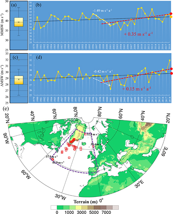
We defined two variables to describe the EECs-associated MSWs during a year: (i) the maximum value of the MSWs within a year was defined as the MMSW, which was used to represent the strongest intensity of the MSWs of the year; and (ii) the average value of the MSWs within a year was defined as the AMSW, which was used to denote the mean intensity of the MSWs. The maximum, mean and minimum of the MMSWs during the 40 year period were 46.7 m s−1, 39.2 m s−1 and 32.3 m s−1, respectively (figure 6(a)), which mainly appeared within the sector (39° N−75° N, 53° W−2° E)(purple dashed sector in figure 6(e)). Most of the MMSWs (∼90%) were located west of 30° W, with only one event appeared east of 0° E. From 1979 to 2018, the MMSW showed an unobvious increasing trend (table 1), whereas, during the recent 20 years (from 1999 to 2018), the MMSW showed a notable increasing trend of 0.35 m s−1 a−1 (figure 6(b)), which passed the Mann–Kendall trend test (p = 0.05).
Figure 6. MMSW = the maximum value of the MSWs within a year; AMSW = the averaged value of the MSWs within a year. Panel (a) is the boxplot of the MMSWs over the PNAA during the 40 year period (m s−1). The box indicates the 25th (Q1) to 75th (Q3) percentiles, the small cross represents the mean value, and the line indicate the median value; the whiskers indicate the range of [Q1 − 1.5 × (Q3 − Q1)] (or the minimum of the data) and [Q3 + 1.5 × (Q3 − Q1)] (or the maximum of the data), and the outliers are shown by small orange circles. Panel (b) shows the annual variation of the MMSW (m s−1), where the black dashed line shows the 40 year linear trend, the red dashed line shows the 20 year linear trend (from 1999 to 2018), and the red value is the 20 year trend. The white dashed line with an arrow head shows the linear trend (from 1996 to 2001), and the white value is its trend. Panel (c) is the same as (a) but for the AMSW; panel (d) is the same as (b) but for the AMSW. The trend exceeding the 95%/90% confidence level (the student's t-test) is highlighted by a red/orange circle. Panel (e) shows the locations (small red boxes) of the MMSWs during the 40 year period, where the purple dashed sector outlines the region for calculate the horizontal mean for the index. All the linear trends exceeding the 95% confidence level also passed the Mann–Kendall trend test (p = 0.05).
Download figure:
Standard image High-resolution image
Table 1. Linear trends of various variables over the North Atlantic Storm track (NAST) during a 40 year period, with those exceeding the 95%/90% confidence level (based on the student's t-test) highlighted in bold red/blue. STE = surface temperature (K a−1); STG = surface temperature gradient (K m−1 a−1); VMO = vertical motion (Pa s−1 a−1); MMSW = the maximum value of the MSWs within a year (m s−1 a−1); AMSW = the averaged value of the MSWs within a year (m s−1 a−1); SPR = spring; SUM = summer; AUT = autumn; and WIN = winter. All the linear trends exceeding the 95% confidence level also passed the Mann–Kendall trend test (p = 0.05).
| MMSW | AMSW | STE | STG | VMO | |||||||||
|---|---|---|---|---|---|---|---|---|---|---|---|---|---|
| SPR | SUM | AUT | WIN | SPR | SUM | AUT | WIN | SPR | SUM | AUT | WIN | ||
| +0.08 | +0.03 | +0.03 | +0.03 | +0.04 | +0.04 | +0.3 × 10⁻⁸ | +3 × 10⁻⁸ | −1.3 × 10⁻⁸ | −1.6 × 10⁻⁸ | −5 × 10⁻⁵ | +2 × 10⁻⁵ | −5 × 10⁻⁵ | −5 × 10⁻⁵ |
The maximum, mean and minimum of the AMSWs during the 40 year period were 32.0 m s−1, 28.8 m s−1 and 26.2 m s−1, respectively (figure 6(c)). From 1979 to 2018, the AMSWs showed a significant increasing trend of 0.03 m s−1 a−1 (table 1), that passed the Mann–Kendall trend test (p= 0.05). During the recent 20 years (from 1999 to 2018), a more rapid increasing trend of 0.15 m s−1 a−1 appeared (figure 6(d)). As mentioned above, the EECs' impacts enhanced in terms of the MSWs, particularly for the recent 20 years, during which, the maximum and average intensity both intensified significantly. For the future, based on the phase 5 of the Coupled Model Intercomparison Project, Seiler and Zwiers (2016) proposed that, over the Atlantic, the total number of EECs was projected to decrease toward the end of the 21st century. However, this did not mean the EECs' MSWs would weaken in intensity, because the EECs were projected to enhance in their intensity in the future over some regions of the Atlantic (Seiler and Zwiers 2016, Kar-Man Chang 2018).
5.2. Indices for estimating the EECs' MSWs
As BEC = −αω was a key factor for producing the EECs' MSWs (section 4.1), we tested whether the VMO could reflect the intensity of AMSW. Since the baroclinic processes in the layer from surface to 500 hPa were crucial for the surface wind (Fu et al 2014, 2018, Jiang et al 2021a), we first calculated the vertical mean of ω in this layer, then calculated its season mean during each year, and finally calculated its horizontal mean within the sector shown in figure 6(e). The result was defined as the index VMO. As shown in table 2, the linear correlation coefficient between the AMSW and the VMO of autumn was −0.49 (exceeding the 99.5% confidence level). This means that stronger AMSW tended to appear within the year when ascending motions were stronger in autumn. The linear regression equation between the AMSW and VMO (autumn) was:

Table 2. The correlations between various variables over the North Atlantic Storm track (NAST) during a 40 year period, with those exceeding the 95%/90% confidence level (the student's t-test) highlighted in bold red/blue. STE = surface temperature, STG = surface temperature gradient, VMO = vertical motion (vertically averaged from surface to 500 hPa), all of which were horizontally averaged within the purple dashed sector shown in figure 6(e). The sign '—' means not calculated.
| MMSW | AMSW | STE | STG | VMO | |||||||||||
|---|---|---|---|---|---|---|---|---|---|---|---|---|---|---|---|
| SPR | SUM | AUT | WIN | SPR | SUM | AUT | WIN | SPR | SUM | AUT | WIN | ||||
| STE | SPR | −0.06 | −0.05 | — | — | — | — | −0.43 | — | — | — | −0.22 | — | — | — |
| SUM | 0.01 | −0.06 | — | — | — | — | — | 0.48 | — | — | — | 0.08 | — | — | |
| AUT | 0.07 | 0.10 | — | — | — | — | — | — | −0.30 | — | — | — | −0.18 | — | |
| WIN | 0.11 | 0.16 | — | — | — | — | — | — | — | −0.37 | — | — | — | −0.04 | |
| STG | SPR | 0.15 | 0.3 | −0.43 | — | — | — | — | — | — | — | 0.53 | — | — | — |
| SUM | 0.15 | 0.32 | — | 0.48 | — | — | — | — | — | — | — | 0.33 | — | — | |
| AUT | −0.09 | −0.14 | — | — | −0.30 | — | — | — | — | — | — | — | 0.65 | — | |
| WIN | −0.09 | 0.05 | — | — | — | −0.37 | — | — | — | — | — | — | — | 0.47 | |
| VMO | SPR | 0.01 | −0.03 | −0.22 | — | — | — | 0.53 | — | — | — | — | — | — | — |
| SUM | −0.18 | 0.02 | — | 0.08 | — | — | — | 0.33 | — | — | — | — | — | — | |
| AUT | −0.18 | −0.49 | — | — | −0.18 | — | — | — | 0.65 | — | — | — | — | — | |
| WIN | −0.07 | −0.31 | — | — | — | −0.04 | — | — | — | 0.47 | — | — | — | — | |
where the unit for VMO was Pa s−1.
Because strong baroclinity was necessary for strong BEC, we tested whether the surface temperature gradients (STGs) could reflect the intensity of the AMSW. We first calculated  , where
  is the horizontal gradient operator and Ts is the surface temperature; then we calculated its season mean during each year, and finally we calculated its horizontal mean within the sector shown in figure 6(e). The result was defined as the index STG. The correlation coefficient between the STG in summer and the AMSW was 0.32 (table 2; exceeding the 95% confidence level), implying stronger AMSW tended to appear within the year when the baroclinity was stronger in summer. The linear regression equation between the AMSW and STG (summer) was:

where the unit for STG was 10−4 K m−1.
As mentioned above, the absolute value of the linear correlation coefficient between the AMSW and the VMO/STG was 0.49/0.32. Then, we combined equations (2) and (3) by their relative importance in linear correlation (i.e. equation (2) * 0.49/(0.49 + 0.32) + equation (3) * 0.32/(0.49 + 0.32)), and we could obtain the following equation:
Equation (4) is a mechanism-based statistical model, which may have the potential to estimate the AMSW over the NAST. Moreover, as the linear correlation coefficient between the MMSW and AMSW during the 40 year period was 0.48, we concluded that, stronger MMSW tended to appear in the year with stronger AMSW.
6. Conclusion and discussion
After nearly a century of studies on the EECs, their MSWs, which possess huge destructive power, are rarely investigated. In this study, we explored the key statistical features of the EECs' MSWs over the NAST and clarified their main formation mechanisms, which partly filled the current knowledge gaps. We found that, much more EECs' MSWs occurred over the ocean than on land, with >75% of the MSWs appeared within 300–800 km from the EECs' centers. Of the EECs' eight octants, O1 and O2 were the most dangerous, because >1/3 of the MSWs appeared here, and the maximum/mean intensity of the MSWs within O1–O2 was the largest among all EECs' octants. For O6 (14.7%), O7 (12.2%) and O8 (8.8%), their accumulated proportion for the MSWs was 35.7%. This was consistent with the results from previous studies, as these case studies found the sting jets appeared within O6–O8 (Clark et al 2005, Clark and Gray 2018). Overall, the EECs' MSWs showed a notable intensity-dependent feature: as the EECs became stronger, their MSWs enhanced in intensity, more MSWs appeared in the regions closer to the EECs' centers, the proportion of MSWs that occurred within O1–O2 increased. The BEC which converted the available potential energy into KE was crucial for generating the EECs' MSWs. The superposition of EECs' moving on the cyclone relative winds exerted notable effects on the intensity/direction of the MSWs, with the MSWs of O6–O8 enhanced, whereas those of O1–O5 abated. The trend analyses show that, over the NAST, the AMSW showed a significant linear trend of increasing during the 40 year period, whereas, that of the MMSW was not significant. This is partly because a significant rapid decreasing in the MMSW (around −1.49 m s−1 a−1) appeared from 1996 to 2001, which made its 40 year trend less significant. In the recent 20 years (from 1999 to 2018), the strengths of the AMSW and MMSW both increased significantly, implying that the risks from EECs' strong winds enhanced notably. Based on the dominant formation mechanisms of EECs' MSWs, we used two indices, i.e. the STG (summer) and VMO (autumn), to develop a statistical model for estimating the annual averaged intensity of the EECs' MSWs.
The resolution of reanalysis data was an important factor when analyzing the EECs' MSWs. To roughly evaluate the effect, we conducted a comparison between the MSWs detected by the 0.75° × 0.75° ERA-Interim and the 0.25° × 0.25° ERA5 reanalysis data (Hersbach et al 2020) during 2018. We found that, on average, the ratio of the MSWs detected by ERA-Interim to those detected by ERA5 was ∼0.9 (not shown). This means that the MSWs detected by the ERA-Interim and ERA5 had a good correlation to each other, with the intensity of the latter larger than those of the former. Therefore, the key statistical features on EECs' MSWs obtained by using both types of reanalysis data should be consistent. However, since the MSWs were stronger for using ERA5, this study might underestimate the MSWs' intensity. We suggest to conduct more studies on the EECs' MSWs by using various types of data in the future, which would result in a more comprehensive understanding of EECs' strong winds.
As proposed by Hart et al (2017), the ERA-Interim reanalysis data is mainly capable of revealing the synoptic-scale winds associated with the extratropical cyclones; whereas, for the sting jet (Martínez-Alvarado et al 2013, Clark and Gray 2018), which is a mesoscale phenomenon, ERA-Interim shows a notable limitation to resolve it. According to Martínez-Alvarado et al (2012), ∼1/3 of the EECs are associated with sting jets. Therefore, for these EECs, we suggest to use the reanalysis data of a higher spatiotemporal resolution or mesoscale numerical simulations for a further research.
Acknowledgments
The authors would like to thank the European Centre for Medium-Range Weather Forecasts for providing the data used in this study (the ERA-Interim reanalysis data can be download at https://rda.ucar.edu/datasets/ds627.0/; the ERA5 reanalysis data can be downloaded at https://rda.ucar.edu/datasets/ds633.0/). This research was supported by the National Natural Science Foundation of China (42075002; U2142202), and the National Key Scientific and Technological Infra structure Project 'Earth System Science Numerical Simulator Facility'.
Data availability statement
The data that support the findings of this study are openly available at the following URL/DOI: https://rda.ucar.edu/datasets/ds627.0/.