

Abstract
Light-duty transportation continues to be a significant source of air pollutants that cause premature mortality and greenhouse gases (GHGs) that lead to climate change. We assess PM2.5 emissions and its health consequences under a large-scale shift to electric vehicles (EVs) or Tier-3 internal combustion vehicles (ICVs) across the United States, focusing on implications by states and for the fifty most populous metropolitan statistical areas (MSA). We find that both Tier-3 ICVs and EVs reduce premature mortality by 80%–93% compared to the current light-duty vehicle fleet. The health and climate mitigation benefits of electrification are larger in the West and Northeast. As the grid decarbonizes further, EVs will yield even higher benefits from reduced air pollution and GHG emissions than gasoline vehicles. EVs lead to lower health damages in almost all the 50 most populous MSA than Tier-3 ICVs. Distributional analysis suggests that relying on the current gasoline fleet or moving to Tier-3 ICVs would impact people of color more than White Americans across all states, levels of urbanization, and household income, suggesting that vehicle electrification is more suited to reduce health disparities. We also simulate EVs under a future cleaner electric grid by assuming that the 50 power plants across the nation that have the highest amount of annual SO2 emissions are retired or retrofitted with carbon capture and storage, finding that in that case, vehicle electrification becomes the best strategy for reducing health damages from air pollution across all states.
Export citation and abstract BibTeX RIS

Original content from this work may be used under the terms of the Creative Commons Attribution 4.0 license. Any further distribution of this work must maintain attribution to the author(s) and the title of the work, journal citation and DOI.
1. Introduction
In the United States, emissions standards set upper limits on emissions per mile for various air pollutants for new vehicles. These standards have helped drastically reduce air pollutants from light-duty vehicles (LDVs). Between Tier 1 (1994) and Tier 3 standards (2017), the allowed NOx (nitrous oxide) and PM2.5 (particulate matter less than 2.5 μm) emissions per mile from gasoline vehicles decreased by more than 90% [1, 2]. However, LDVs continue to contribute to 10% of the total PM2.5 attributable premature mortality, with disproportionate impacts on people of color and minorities [3–5]. Historical race-based housing segregation and land-use practices like building freeways through communities of color perpetuate these systemic transportation inequalities despite massive improvements in overall air quality [3, 6]. Studies have shown people of color are consistently exposed to higher concentrations of NO2 (a marker for traffic pollution) than White people [7, 8]. Reduction in traffic congestion with the introduction of electronic tolls has reduced premature mortality by ∼8% and low birth weight among mothers by ∼10%, with larger benefits for African Americans [9]. On the climate front, the transportation sector leads in total greenhouse gas (GHG) emissions in the U.S. (1.7 billion metric tons per year), with LDVs contributing to 58% of the total transportation-related emissions [10].
Primary PM2.5 emissions from gasoline internal combustion vehicles (ICVs) include tailpipe emissions, dust re-suspension, and tire and brake wear. Secondary PM2.5 is also formed due to chemical reactions of precursor species such as nitrous oxides (NOx ), non-methane organic gases (NMOGs—a subclass of volatile organic oxides comprising of non-methane hydrocarbons and oxygenated hydrocarbons), and ammonia [2]. Emissions standards set a quantitative limit of pollutant emissions that new vehicles can emit per mile. The first set of standards, called Tier 1 standards, were phased in between 1994 and 1997, followed by Tier 2 standards between 2004 and 2009. Tier 3 standards were finalized in 2015 and will be phased between 2017 and 2025. The standards have been tightened considerably: per-mile gasoline NOx + NMOG and PM2.5 limits under regulatory test conditions have decreased by 91% and 97%, respectively, between 1994 and 2022. In SI section S.2a, we provide more details on how the standards for different pollutants, vehicles, certification bins, and test procedures have evolved.
Under Tier 3 standards, manufacturers need to adhere to emissions limits under laboratory testing conditions for their total annual sales as well as for each vehicle. Tier 3 standards introduced a limit on per mile NMOG + NOX emissions instead of limits of NMOG and NOx individually, as was done previously. The standard also includes per-mile limits for PM2.5, carbon monoxide (CO), and formaldehyde [2]. Manufacturers can balance NOx + NMOG emissions across individual vehicles sold in a year as long as the new-sale fleet-wide emissions standard is achieved. Each vehicle is required to attain the PM2.5 emission standard. Standards also depend on the driving conditions they are tested on. Federal Test Procedure or FTP simulates city driving conditions, US06 approximates high acceleration aggressive driving, and supplemental FTP is a mixture of city driving, aggressive driving, and driving with air conditioning (SI section S.2a) [11]. For this work, we consider FTP and SFTP emissions standards as two scenarios for Tier-3 ICVs. New vehicles on the road generally emit below the emissions standards [12, 13], but in the past, some manufacturers have used defeat devices to disable emissions controls under real-world driving [14]. Also, vehicle emissions per mile increase significantly with age and cumulative mileage [15–21].
Electric vehicles (EVs) have emerged as another alternative. EVs can reduce transportation-related air pollution, associated inequities, and GHG emissions under a low-emitting electricity grid. PM2.5 health damages from EVs depend on the emission intensity of the electricity used to charge them. Vehicle charging demand, which constituted only 11 out of 4116 TWh of electricity demand [22, 23], will significantly increase with rising EV penetration. Total electricity generation in the U.S. was associated with ∼16 400 PM2.5 premature deaths in 2014, with Black and White people experiencing higher premature mortality. Coal power plants were responsible for ∼93% of electricity PM2.5-related premature mortality in the U.S [24]. Hence, coal retirements will be crucial to reducing the health impacts of large-scale EV transition.
Previous work has found that EVs powered by low-emitting electricity reduce health impacts by 50% compared to conventional gasoline vehicles. In comparison, those powered by coal-based or the then 'grid-average' emissions intensity increase damages by 80% [25]. Hence, reducing upstream air emissions from electrified transportation will require reducing air emissions from the power sector. This shift will have different consequences across the country, given the different composition of electricity generation. Several studies have compared the health damages of transportation technologies in the US using a marginal damages approach, wherein an incremental vehicle mile traveled (VMT) is small enough to be treated as marginal, and damages are calculated as the product of emission factor (emissions per mile) and marginal damages of a pollutant [26]. Using a marginal damages approach, Tong and Azevedo find that in the Western US and New England, switching to an EV would reduce monetized damages when compared to gasoline vehicles, whereas gasoline hybrid vehicles would be less damaging in the Midwest [27]. Choma et al show that EVs have less health damages than ICVs in all U.S. metropolitan statistical areas (MSAs) [28]. Holland et al calculate the net environmental benefits of vehicle electrification, finding those to be positive for Asian and Latino Americans (data from 2010 to 2014) [29, 30]. Other studies have used chemical transport models to estimate air quality and distributional equity consequences of LDV electrification to find similar conclusions. PM2.5 changes due to electrification depend on the source and location of electricity generation used to charge electric vehicles. EVs increase pollution in areas close to coal power plants [31] but reduce pollution in urban regions [32, 33] and in states with low-carbon electricity like California [34]. Peters et al [35] estimate health benefits and avoided mortality at 25% and 75% EV adoption with three different electricity grid scenarios, including the current grid and a future low-emissions one. The highest health benefits are achieved with a low-emitting grid, and increasing EV adoption without reducing emissions from the grid only provides small health benefits. The composition of electricity generation, the concentration of local air pollutants, and vehicle technologies have changed substantively since these previous studies were published. For example, the per-mile emissions from Tier 3 vehicles for NOX , PM2.5, and volatile oxides are 96%, 80%, and 95% smaller than those of the current LDV fleet (table 1). EVs and the electricity sector have also evolved. Since 2015, the range of new EVs has increased by 9%, and coal-generated electricity has been reduced by 30% [36, 37].
Table 1. Scenarios considered for Tier-3 ICVs.
| Scenario | Drive cycle | NOX + NMOG (mg/mile) | NOX /NMOG ratio | PM2.5 (mg/mile) |
|---|---|---|---|---|
| 1a | FTP | 51 | 50/50 | 3 |
| 1b | SFTP | 70 | 50/50 | 10 |
| 1c | FTP | 51 | 70/30 | 3 |
| 1c | FTP | 51 | 30/70 | 3 |
In this work, we estimate PM2.5 related health impacts and change in socio-economic disparities associated with four scenarios: (i) a business-as-usual, reflecting the current LDV fleet; (ii) a replacement of the current LDV fleet with gasoline vehicles that meet the model year 2022 Tier 3 emissions standards, (iii) replacement of the current LDV fleet with a range of EV models charged with the current electricity grid, and (iv) replacement of current LDV fleet with a range of EV models charged with a future clean electricity grid where 50 power plants with the highest SO2 emissions have been retired or retrofitted with carbon capture and storage (CCS). In post-combustion CCS, SO2, NOx , and PM2.5 are removed from the flue gas before CO2 is captured and removed [38].
We use a reduced complexity air quality model (InMAP) [39] to estimate the change in PM2.5 concentration due to changes in emissions from point sources (power plants) and area sources (gasoline ICVs) across the U.S [40]. Reduced complexity air quality models (RCM) have become a popular tool in recent years to evaluate the air quality implications of different policies or technologies [4, 24, 25, 29, 30, 41–44]. Some widely used RCMs include InMAP, AP3, and EASIUR [39, 45–47]. Previous research has shown that the three RCMs produce marginal damages within the same order of magnitude despite structural differences. For example, for ground-level primary PM2.5, the models have very similar values across all counties, with Pearson's correlation ranging from 0.73 to 0.81. Benchmarking studies also indicate that RCMs can be used instead of chemical transport models for scenario modeling with only a modest loss of accuracy [48, 49].
We use local air pollutant emissions and emissions of GHGs from the electricity sector [40, 50, 51]. For Tier-3 ICV, we use Tier-3 emission standards for model year 2022 in FTP and SFTP test conditions [1, 2]. We use census block group data (ACS 2019–2020) [52, 53] as a source of information for demographic characteristics. We use our previous estimates of the energy needed to charge EVs in different locations, which account for ambient temperature conditions, drive cycle (city, rural, or combined), vehicle make, and model [54].
The rest of this paper is organized as follows: we describe data and methods used for the analysis, followed by air quality and climate change impacts of the fleet-wide use of EVs and Tier-3 ICVs. We assess equity implications across different socio-economic aspects and conclude with findings and recommendations. The key contribution of this work is to assess how less polluting conventional vehicles (Tier-3 ICVs) would fare when compared to electric vehicles in terms of air pollution and distributional equity across the nation. While past studies have detailed the increasing stringency of emissions over time [21, 55] and their positive impact on air quality [56–58], our work incorporates Tier-3 vehicles and provides important regional conclusions.
2. Methods and data
We estimate impacts on climate change and PM2.5-related health and socio-economic disparities associated with the following scenarios: (i) a business-as-usual scenario, where we compute the health damages from the current fleet of LDV across the U.S.; (ii) a replacement of the current fleet with gasoline vehicles that meet the strictest emissions standards (Tier-3 ICV), and (iii) a replacement of the current fleet of LDVs with electric vehicles that are charged with the current grid and (iv) a possible future low-carbon electricity grid where 50 plants with highest annual SO2 emissions are retired or retrofitted with CCS. We estimate health impacts from these scenarios by race, ethnicity, geography, and income for states in the contiguous United States and for the 50 most populous MSAs. Throughout this work, health consequences refer to the attributable premature mortality associated with the increase in PM2.5 concentration associated with primary PM2.5 emissions and precursor pollutants, such as SO2 and NOx , from the different transportation technologies studied in this paper.
There are three modeling steps in our methods. Firstly, we estimate annual tailpipe emissions from ICVs (Tier-3 and current fleet) at the census tract level. These emissions are treated as ground-level area source emissions, i.e. the annual emissions of each pollutant are assumed to be uniformly distributed across the census tract (SI sections S.1 and S.2). InMAP, the reduced complexity air quality model used in this work, allocates these input emissions to model cells using area weighting (SI section S.5c) and converts pollutant emissions to changes in PM2.5 concentration. The grid cell size in InMAP varies depending on population density (figure 1), with the largest grid cell of 48 km × 48 km in sparsely populated regions and 1 km × 1 km in densely populated urban areas. Pollution from electric vehicles is attributed as an increase in emissions proportional to the increase in electricity generation due to electric vehicle charging demand. Emissions from power plants are treated as point sources in a specific InMAP grid cell, and the change in PM2.5 concentration is estimated for all power plants. After estimating the change in PM2.5 concentration due to each technology choice, we spatially overlay the census block group with InMAP grid cells to find the counts of the total population and population of races and ethnicities exposed to the change in PM2.5. Using a concentration-response function, total premature deaths are calculated at the census block group level. Mortality rate (deaths per 100 000 people) is reported at two aggregation resolutions—MSA level and state level. State level captures the heterogeneity in transportation and electricity emissions and provides analysis to sub-national decision-makers regarding EV adoption policies.

Figure 1. Modeling steps and spatial resolution of inputs, outputs, and post-processing used in this work.
Download figure:
Standard image High-resolution image2.1. Assumptions regarding driving patterns
For all scenarios, we use estimates of VMT at the census tract level using multiple data sources [40, 59, 60] and as explained in detail in SI section S.1. We assume that census tract level miles driven are the same across scenarios. In the SI section S.6c, we also run our analysis using county-level emissions as the National Emissions Inventory, one of our primary sources of emissions from the current LDV fleet, reports total emissions at the county level and discuss the differences in the results. Across all scenarios, dust suspension and tire break-and-wear emissions of ICVs and EVs are not included. However, emerging evidence shows EVs may have smaller brake wear emissions due to regenerative braking but larger tire wear emissions due to higher weight [61, 62]. Internal combustion engines equipped with selective catalytic reactors are an emerging source of ammonia due to 'ammonia slipping,' which occurs due to non-optimal temperatures in the exhaust chamber [63–65]. We do not include this effect in the main results as emissions standards currently do not regulate ammonia, but it could be an emerging source of secondary PM2.5.
2.2. Census data
We use population, race, and ethnicity data from ACS 2016–2020, obtained via NHGIS IPUMS [53]. We use eight racial-ethnic groups. People who self-identify as Hispanic or Latino ethnicity are included here as Latino (all races). The seven racial groups in ACS (i.e. Black, White, Asian, Native American & American Indian (Native), Hawaiian & Pacific Islander (HPI), Other, and Mixed here refer to non-Hispanic individuals.
Census block group-level population data are distributed to the InMAP grid as an area-weighted average (figure 1). The total population is 324.41 million, out of which 195.5 million are White, 59.1 million are Hispanic/Latino, 39.94 million Black, 17.6 million Asian, 8.8 Mixed, 1.96 million Native American and American Indian, and 0.4 HPIs.
2.3. Baseline: characterization of the current LDV transportation fleet
National Emissions Inventory (NEI 2017) reports that total on-road non-diesel LDVs drove 2.65 trillion miles, emitting 1.9 million short tons of nitrogen oxides (NOx ), 1.5 million short tons of VOCs, and 0.05 million short tons of primary PM2.5 [40]. We use county-level emissions of NOx , NMOG (VOC), and primary PM2.5 reported by NEI and redistribute them to census tracts based on VMT estimates described above to model the health consequences of emissions as our current LDV fleet. Ammonia emissions for the current LDV fleet are not included in the analyses in the main text to enable comparison with emissions standards that do not regulate ammonia. Change in pollution exposure with changes in emissions is modeled using InMAP, a reduced complexity air quality model.
2.4. Scenario 1: fleetwide adoption of gasoline Tier-3 ICV
Emissions standards set quantitative limits of pollutant emissions that new vehicles can emit per mile. Between Tier 1 (1994) and Tier 3 standards (2022), per-mile gasoline NOx + NMOG and PM2.5 limits under regulatory test conditions have decreased by 91% and 97%, respectively. For this work, we rely on model year 2022 Tier 3 emissions standards in the FTP drive cycle and supplemental FTP drive cycle as two possible scenarios (SI section S2a). We use fleet-wide average emissions standard values for NOX and NMOG. Since Tier 3 standards regulate total NOx + NMOG emissions, we assume different ratios of NOX and NMOG (50:50, 30:70, or 70:30) to account for uncertainty [66] (SI sections S2b and S6b). We assume that all vehicles meet the PM2.5 mandated standard. Because the emissions of new Tier 3 vehicles will change with age and cumulative mileage, our estimates represent a lower bound of health damages for ICVs. Table 1 shows the emissions per mile for Tier 3 emissions standards (model year 2022) on FTP and SFTP drive cycles with different NOx and NMOG ratios.
2.5. Scenario 2: fleetwide adoption of electric vehicles
We use results from previous works to estimate a range of electricity consumption if the entire existing stock of vehicles were to be substituted by electric vehicles [54]. In brief, the energy consumption of electric vehicles is significantly impacted by both temperature and type of driving. We estimate the electricity required by an electric vehicle by using publicly available laboratory-tested data on energy consumption per mile at different temperatures, drive cycles, and vehicle miles traveled, as described above. Our estimates account for the effect of hourly ambient temperature at the county level and whether the type of driving in a county is predominantly city, highway, or combined driving. We use the Nissan Leaf (economy car, 40 kWh battery) and the Tesla Model S (luxury car, 100 kWh battery) as reasonable low and high bounds of the energy requirements of EVs (SI section S.3a) [67]. We assume vehicles are charged with the fleet of electricity generators in their NERC regions (SI section S.5b). NERC regions roughly divide the contiguous United States into six regional reliability entities and differ in power systems characteristics and resources. In table 2, we report the range of average energy requirements for Nissan Leaf and Tesla Model S across counties in different NERC regions, as estimated in our previous work, and the rough geographic representation of each NERC region by sub-regions of the United States.
Table 2. Electricity requirements for vehicle electrification.
| NERC region | Sub-region represented in the continental United States | Electricity generated in the NERC region in 2019 (TWh) | Average energy requirement of short-range and long-range EV in sample per 1000 vehicle-miles (kWh) | Total electricity requirement from converting the fleet (TWh) |
|---|---|---|---|---|
| MRO | Upper Midwest and Great Plains | 448 | 326–396 | 52–68 |
| NPCC | New York + New England | 231 | 312–406 | 68–93 |
| RFC | Great Lakes | 918 | 306–401 | 170–228 |
| SERC | Southeast and Florida | 1,354 | 296–379 | 233–306 |
| TRE | Texas | 414 | 292–365 | 49–65 |
| WECC | Rocky Mountain, Southwest, and Pacific Coast | 738 | 317–396 | 167–223 |
We assume the electricity generated to meet the electricity demand from charging the vehicles will be distributed across power plants proportionally to their annual 2019 generation. We ignore the potential redispatch of power plants due to the demand for EV electricity. We also do not account for potential electricity generation capacity limits for a plant that may occur at high charging levels or for marginal generator characteristics. This assumption is suitable given that we are considering scenarios where many vehicles are being replaced, and we are using annual emissions from the electricity grid. We estimate plant-level emissions of SO2, and NOX using NEI 2017 and primary PM2.5 e-GRID 2019 data [40, 50, 68]. Our dataset includes 3342 fossil power plants out of a total of 3400. Our estimates of total emissions are 0.13 million short tons for PM2.5, 1.08 million short tons for SO2, and 1.16 million short tons of NOx . We exclude from our analysis 30 renewable plants that have a small percentage of oil, coal, or gas. To our knowledge, this is the most exhaustive and up-to-date characterization of the current electricity system for evaluating air pollution-related health impacts.
For our analysis of the future clean grid where 50 most SO2 polluting power plants were retired or retrofitted with CCS, we assume that they are either replaced by renewable energy or did not have a reduction in their generation due to CCS. All retired or retrofitted plants in the continental US, except one, are coal power plants (SI section S.3d). These 50 power plants constituted 78 GW in nameplate capacity, 335 TWh of generation, and emitted 253 kilotons NOx , 663 kilotons SO2, 20 kilotons PM2.5, and 364 447 kilotons CO2 emissions. For context, cumulative wind and solar capacity in the US are nearly 136 GW and 73.5 GW [69, 70] and 300 GW of wind and 947 GW of solar are currently in transmission interconnection queues [71]. A complete list of power plants, state-wise capacity, generation removed or retrofitted, and emissions avoided are given in SI section S.3d.
Table 3 shows the total electricity generation in each NERC region, the percentage of renewable generation, and the total emissions of SO2, NOx and, PM2.5, and CO2 for 2019 (more details in SI sections S.3b and c).
Table 3. Total electricity generation (TWh) and total pollution emissions in NERC regions (2019).
| NERC region | Electricity generation (TWh) | SO2 (tons) | NOx (tons) | PM2.5 (tons) | CO2 (million tons) | Percentage of renewable generation |
|---|---|---|---|---|---|---|
| MRO | 448 | 175 209 | 160 380 | 12 684 | 232 | 34 |
| NPCC | 231 | 8,227 | 30 046 | 4,764 | 49.2 | 25 |
| RFC | 918 | 286 512 | 289 743 | 38 741 | 443 | 6 |
| SERC | 1,354 | 369 212 | 321 104 | 46 632 | 618 | 7 |
| TRE | 414 | 118 936 | 106 874 | 9,525 | 180 | 20 |
| WECC | 738 | 98 667 | 216 045 | 16 548 | 284 | 39 |
2.6. Modeling the change in PM2.5 concentration
We use InMAP, a reduced complexity air quality model [39, 45] to estimate the change in concentration of PM2.5 across our different scenarios. InMAP uses an Eulerian grid model to estimate the annual average PM2.5 concentration change attributed to a change in annual emissions based on steady-state solutions to equations representing pollution emission, transport, transformation, and removal. InMAP's representation of chemistry and meteorology uses spatially varying parameters obtained from a detailed chemical transport model simulation (the WRF-Chem model coupled with the National Emission Inventory). The InMAP source-receptor matrix (ISRM) provides a relationship between source damages (i.e. damages across the country that are attributable to emissions in a specific grid cell) and receptor damages (i.e. the damages suffered by people in a particular grid cell, regardless of where the emissions occurred). This ISRM was built by running more than 150 000 runs of InMAP, each time inputting a 1-t emission change from a single grid (out of ∼50 000 grid cells) at three different heights (ground, medium, and high height). ISRM as a dataset contains estimates of a linear relationship between marginal changes in emissions at every source location and marginal changes in annual-average PM2.5 concentration at a receptor location [44, 72]. The grid-cell size in InMAP varies from 1 km × 1 km (typically in urban areas) to 48 km × 48 km (typically in rural areas), depending on the gradient in the population density and pollutant concentrations. Fine grid in populated areas is critical to accurately estimate air pollution-related health disparities [43, 73]. Our study explicitly looks at receptor damages (where the damages occur) along with a granular characterization of where damages originate (sources).
2.7. Estimating health damages due to PM2.5
Premature mortality due to PM2.5 concentration changes is calculated using the county-wide hypothetical 'underlying incidence,' the mortality hazard ratio derived from the concentration-response function, and the population in the grid cell. We use the approach of Apte et al [74] to calculate the hypothetical underlying incidence rate if there were no PM2.5 emissions,  as:
as:

where  is the reported county-level all-cause mortality,
  , is the average mortality hazard ratio caused by PM2.5 in county c.
  , in turn, is calculated as:
where  is the population in grid cell i; n is the number of grid cells in county c;
  is mortality hazard ratio (GEMM in this study) resulting from ambient PM2.5 concentration
  i, and
  is the area fraction of grid cell i that overlaps with county c. We use ambient PM2.5 concentration from Meng et al for 2019 [75]. The authors estimate ambient PM2.5 concentration using chemical transport modeling, satellite remote sensing, and ground-based measurements. We use baseline population-wide all-cause mortality rates at the county level from the US Center for Disease Control (CDC) [76] for 2019. Our unit of analysis is limited to the county level as this is the smallest geographic unit with publicly available health data from the CDC. While this CDC data has been used extensively in studies to examine health outcomes and environmental disparities in disadvantaged communities [77–79], health data at finer spatial resolutions would increase the certainty and accuracy in exposure and health disparity estimates. Unfortunately, there is no such data in a publicly available form. The average mortality rate
  is 833.71 deaths per 100 000 people per year, and our
  estimate is 790 deaths per 100 000 people per year (SI section S5d).
Throughout this work, we use the mortality hazard ratio  function from the Global Exposure Mortality for non-accidental mortality (GEMM) to calculate both the underlying incidence rate mentioned above and change in premature mortality due to change in PM2.5 concentration from our scenarios. Non-accidental mortality in GEMM corresponds to non-communicable diseases and Lower Respiratory Infections and uses data from 41 cohort studies from 16 countries to estimate the shape of the association of ambient PM2.5 exposure and non-accidental mortality. GEMM function is supralinear at lower concentrations, near linear at high concentrations, and applies a counterfactual threshold of 2.4 μg m−3, the lowest concentration observed in any of the cohort studies. GEMM function assumes that PM2.5 exposure does not affect health below this level. Some versions of the GEMM function are parameterized differently depending on whether the function is segmented by age and whether a cohort of Chinese men with a wider PM2.5 exposure range than the other studies is included. Our version applies a single function to estimates of non-accidental mortality for all ages above 25 and includes the Chinese male cohort [80]. We use GEMM's equation that uses non-accidental mortality for all ages, which is as follows:
where  is the hazard ratio of mortality incidence at PM2.5 concentration
  in units of micrograms per cubic meter—compared with a hypothetical underlying incidence rate,
  in the absence of ambient PM2.5. Comparison of GEMM with other dose-response functions is given in SI section S.4.
Mortality associated with the concentration of PM2.5 in a grid cell is computed as:
where  are premature deaths caused by the concentration of PM2.5 at location i,
  is the population in grid cell i,
  underlying incidence rate for one
  counties overlapping grid
  and
and  is the fraction of grid cell
  that overlaps county
  .
.
The transportation-attributable mortality rate is aggregated at the state and MSA levels as follows:
3. Results
3.1. Switching the U.S. LDV fleet to EVs or Tier-3 ICVs reduces premature mortality from air pollution in all states and metropolitan statistical areas (MSA)
For results across different scenarios, the concentration-response function, all-cause mortality, the underlying incidence rate, and the population counts remain the same. The changes in premature mortality are only due to changes in air emissions from different transportation choices. Tier-3 ICVs and EVs reduce total mortality by 80%–92% compared to the current fleet (SI section S6b). While the underlying assumptions and risk function differ, our estimates of premature mortality due to electric vehicles are in agreement with the most recent study by Peters et al [35]. We also present changes in PM2.5 exposure from different transportation choices in SI section S6a.
The health benefits are particularly large for states and MSAs with large populations. Figure 2(a) shows the state-wide mortality rate of the current LDV fleet compared to two alternative scenarios: a fleet-wide transition to Tier-3 ICVs and EVs charged on the current electricity grid. Estimates for Tier-3 ICVs may, in practice, be higher in real-world conditions and will increase with age and cumulative mileage. In the future, electric vehicle emissions will be lower than our estimates suggest since the grid is expected to continue decarbonizing.

Figure 2. Comparison of mortality (deaths per 100 000 people) (a) and total CO2 emissions (million tonnes) (b) due to Tier-3 ICVs and EVs charged on the current grid compared to the current LDV fleet by state. States are arranged in decreasing order of current LDV mortality by census region. Mortality ranges for Tier-3 ICVs are given by FTP and SFTP drive cycle with an assumed ratio between NOX and NMOG of 1:1. In contrast, mortality ranges for EVs are given by whether the fleet-wide electrification is done through a low-range Nissan Leaf or a high-range luxury Tesla Model S. CO2 emissions from ICVs are estimated using the CAFE standards for the year 2021 and 2022 and EV CO2 emissions are calculated using the state Power Sector Index of 2021 as outlined by [75, 76] along with data on miles driven and energy consumption details given in methods and data. The two columns on the secondary Y axis show the state population (100 000 people) and state power sector carbon intensity [75].
Download figure:
Standard image High-resolution imageBlack circles and squares indicate Tier 3 emissions standards for FTP and SFTP driving schedules, respectively, with a ratio of 50:50 between NOx and NMOG. Red and maroon circles indicate the mortality attributable to low-range and high-range EVs, respectively. The energy efficiency of EVs is calculated using temperature and urbanization level characteristics at the county level, as described in our previous work [54]. The carbon intensity of electricity for each state is obtained from the Power Sector Carbon Index [81, 82]. In figure 2(b), we show estimates of CO2 emissions from the current LDV fleet, of Tier-3 ICVs (gray bars), and of the EVs considered in this study, using fuel economy of the latest Corporate Average Fuel Economy (CAFE) standards for passenger cars and trucks for 2021 (46.1, 32.6 MPG) and 2022 (48.2, 34.2 MPG) [83] and the fuel economy of current LDV fleet (23 MPG) [84].
We assume that the vehicle miles traveled are constant for both technologies and are derived from NEI 2017, as explained in the methods and SI section S.1. The secondary Y-axis in subfigures indicates the size of the population of each state (2019) [52] and state's power sector carbon intensity (2021) [82]. The states are ordered based on the decreasing mortality attributable to the current LDV fleet for each census region, i.e. South, Midwest, West, and Northeast (SI section S.5a). In the Western US, EVs have a lower mortality rate than Tier-3 ICVs, except for Wyoming, which still relies on a significant coal fleet. In the Northeast, EVs have similar health damages to Tier-3 ICVs in all states except Pennsylvania. In the Midwest, EVs have higher mortality than Tier-3 ICVs in most states, particularly in the Ohio Valley. In the Southern US, EVs have higher mortality rates than Tier-3 ICVs in most states but perform better in populous states like Florida, Texas, and Georgia. Altering NOX/NMOG ratios to 70:30 from 50:50 did not significantly change the results, with a 3% increase in total deaths (41 deaths). On the other hand, EVs have lower CO2 emissions in all states except West Virginia (state carbon intensity of 876 gCO2/kWh) (figure 2(b)). Removing or retrofitting 50 most SO2 plants achieves health damages parity between EVs and Tier-3 ICVs for almost all states except West Virginia and Kentucky (figure 3).
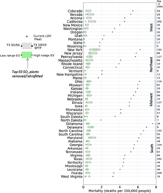
Figure 3. Comparison of mortality (deaths per 100 000 people) for Tier-3 ICVs and EVs charged on a future decarbonized grid where 50 power plants with the highest SO2 emissions are retired or retrofitted with carbon capture and storage (CCS). Post-combustion CCS necessitates the removal of pollutants in flue gas, which include SO2, NOx , and PM2.5.
Download figure:
Standard image High-resolution imageFigure 4 compares damages from changing the US LDV fleet to EVs and Tier 3 ICVs for the 50 most populous MSAs in the U.S. 55% of health damages (∼9 k out of 16 k deaths) from the current LDV fleet occur in the 50 most populous MSAs. Fleet-wide change to Tier-3 ICVs and EVs reduces mortality in all. EVs provide more health benefits than Tier 3 standards in all MSAs except for a few MSAs in the Ohio River Valley (figure 4(a)), where power plants are the predominant source of PM2.5 [85, 86]. A future decarbonized grid can reduce electrification mortality in the region (figure 4(b)).

Figure 4. Mortality (deaths per 100 000 people) associated with passenger transportation for the 50 most populous U.S. MSAs under different scenarios: (i) the current LDV fleet, (ii) a Tier 3 ICE fleet, and (iii) EVs charged on the current grid (orange, figure 4(a)) and (iv) EVs charged on a future grid where the top 50 SO2 polluting power plants are replaced or retrofit with CCS (green, figure 4(b)). We assume a Tier 3 FTP and SFTP drive cycle with a 1:1 ratio between NOX and NMOG. The range of values for EVs corresponds to Nissan Leaf and Tesla Model S. The column on the secondary Y axis shows the state population (in 100 000 people).
Download figure:
Standard image High-resolution image3.2. Demographic differences and risk gap
Figures 5 and 6 present data on passenger vehicles' state-level mortality rates by race and ethnicity across scenarios. Bar height represents the US-wide population average mortality rate for each racial and ethnic group, while black lines indicate the population-level mortality rates by state. Previous research has shown that the current LDV fleet has a greater impact on people of color than on White Americans, with Blacks, Latinos, and Asians experiencing higher mortality rates than the population average [5, 29, 42, 87]. Our estimates are consistent with these earlier findings. Mixed-race also have higher mortality rates than the population average, while Hawaiian and Pacific Island groups have lower. Tier 3 vehicles reduce mortality rates across all groups, but differences between racial and ethnic groups persist. EVs have lower relative disparities than ICVs (figures 6 and 7). White Americans, on average, face higher health consequences than the population average for electric vehicles charged on the current grid, particularly in states in and near the Midwest (Pennsylvania, Indiana, Illinois, Virginia, Maryland) (figure 6, SI section S.6d). Black and Mixed-race Americans also face higher mortality than the population average with EVs charged on the current grid. With a future grid, Black and Mixed-race Americans continue to face higher mortality compared to the population average, but the relative disparity for White Americans declines. Latinos, the second largest ethnic group in the US, face lower transport-attributable mortality compared to the population average with electrification, both with current and future electricity grids (figure 6).
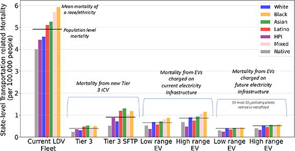
Figure 5. State-level transportation-related mortality rate for current LDV fleet, Tier 3 ICV, EVs charged on current and future electricity grid where 50 power plants with highest SO2 emissions are retired or retrofitted with CCS. The height of the individual bars denotes the population average mortality of each race and ethnicity across all states in the U.S. In contrast, the black lines denote the population's average total mortality rate. The mortality rate is defined as the deaths of a particular race or ethnicity or overall population in the state divided by the population of a race or ethnicity or the total population in the state multiplied by 100 000.
Download figure:
Standard image High-resolution image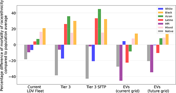
Figure 6. Percentage difference between the mortality of a race/ethnicity compared to the population average mortality for current LDV fleet, Tier 3 ICVs, EVs charged on the current grid, and a future grid where 50 power plants with the highest SO2 emissions are retired or retrofitted with CCS.
Download figure:
Standard image High-resolution image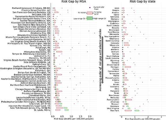
Figure 7. Risk gap of the current LDV fleet compared to Tier-3 ICVs and EVs charged on the current grid. The 50 most populous MSA (figure 7(a)) and states (figure 7(b)) are arranged in increasing order of risk gap for EVs. The risk gap is the difference between the highest mortality of a race or ethnicity and the population mortality for the states or MSA.
Download figure:
Standard image High-resolution imageTo further explore the potential of each technology to reduce pollution disparities, we show the risk gap for states and MSAs in figure 7. The risk gap is the difference between the mortality rate of the most burdened race or ethnicity and that of the overall population of a state or MSA. It is a race-agnostic term used only to capture the differences in pollution disparities between transportation choices. The states and top 50 most populous MSAs are arranged in increasing order of risk gap for EVs. The risk gap decreases with fleet-wide shifts from the current fleet to either Tier 3 ICVs or EVs. An overall switch to EVs (current grid) leads to a lower or almost comparable risk gap with a few exceptions (St. Louis, New York, Houston, and Cincinnati MSAs, and Wyoming, Arkansas, Delaware, West Virginia, and New York states).
3.3. The benefits from electrification or moving to Tier-3 ICV by urbanization and income
Electrifying transportation moves the air pollution from the tailpipe in urban areas to smokestacks of power plants, usually located in areas far from cities [24]. Our results show that while EVs and Tier 3 ICVs both reduce transportation-attributable mortality, they affect rural and urban populations, races and ethnicities, and income groups differently. Figure 8 displays the dependence between income and transport-related mortality categorized by various races and ethnicities for urban and rural populations. The mortality rates are compared across the median household income data for census tracts from ACS 2016–2020 for the current LDV fleet (top row), full electrification using a high-range EV charged on the current grid, and Tier 3 vehicles (FTP drive cycle, 50/50 ratio assumed). The colored lines and marker size correspond to race/ethnicity and their population in the income brackets, and the black line represents the population's average mortality rate. Tracts with a population density above 500 per square mile are defined as urban, while those less are rural as per the 2020 Census urban areas criteria [88].

Figure 8. Transport attributable premature mortality for current LDV fleet, high-range EVs charged on the current grid, and tier 3 ICV dependence on median household income in rural and urban census tracts. Census tracts with a population density of more than 500 per square mile are characterized as urban. Note different Y-axis limits.
Download figure:
Standard image High-resolution image
Both technologies reduced mortality rates for all income groups, races, and ethnicities compared to the current fleet. White Americans have lower mortality compared to the population average in all scenarios except in low-income census tracts. Transport-attributable mortality decreases with increasing income for Asians in urban areas. However, similar trends do not hold for Black and Latino Americans, who see an increase in mortality with income, with a striking increase in urban areas. Our results suggest that within richer urban census tracts, Black and Latino residents have significantly higher transportation-attributable pollution mortality than the population average. Latinos in rural low-income census tracts, though not in high numbers, have disproportionately high mortality with conventional vehicle technologies. Similar figures for tier 3 ICVs on SFTP drive cycle and high-range EVs charged on the future grid where the top 50 SO2 polluting plants are retired are available in SI section S6e.
4. Discussion
This study examines whether using electric vehicles and Tier 3 gasoline vehicles can reduce fleet-wise mortality and disparities associated with transportation-related health impacts and GHG emissions. The current light-duty fleet is an important source of premature mortality due to PM2.5 emissions, especially in urban areas. 55% of health damages (∼9000 deaths out of 16 000) due to the current LDV fleet occur in the 50 most populous MSAs. A transition to EVs and the most efficient Tier 3 ICVs can substantially reduce the health damages from air pollution associated with the transportation sector. Under the current electricity grid, a fleet-wide shift to EVs improves health outcomes in many states and most MSAs compared to Tier-3 ICVs, suggesting that rapid electrification in those locations will be the best health and environmental benefits strategy. Retiring or retrofitting the 50 most polluting coal power plants closes the current gap of health consequences between EVs and Tier-3 ICVs. Lastly, EVs reduce pollution exposure disparities in most states and MSAs.
EVs have lower or comparable mortality to Tier-3 ICVs in the four most populous states—California, Texas, New York, and Florida, although in New York, EVs have a higher risk gap than Tier-3 ICVs. Electrification benefits on current electricity would be delayed for the Ohio Valley region and neighboring states, which includes Kentucky, West Virginia, Pennsylvania, Ohio, and Indiana, owing to the high number of operational coal power plants that currently contribute significantly to ambient PM2.5. Retirement or CCS retrofit in 50 power plants with the highest SO2 emissions can achieve the required air quality parity between EVs and Tier 3 ICVs in this region, except in West Virginia and Kentucky, which will require further pollution reduction.
If the country continues to rely on gasoline vehicles, a move towards Tier 3 vehicles would provide large benefits regarding air pollution damages from passenger vehicles. We note, however, that this ignores another damage associated with gasoline vehicles: the emissions of GHGs that lead to climate change. Furthermore, real-world emissions from these Tier 3 vehicles may deviate from laboratory-tested conditions, and vehicle emissions increase with age and mileage.
Our work has a few limitations. Firstly, while InMAP improves spatial granularity of reduced complexity chemical transport modeling, it cannot capture hyperlocal impacts of transportation-related air pollution, such as near-source proximity to freeways, and emissions can drastically vary within a small geographic region [89]. Secondly, our concentration-response function and the underlying mortality rate are assumed to be the same across races and ethnicities. New studies show there could be differences [90]. Thirdly, this work does not take into account ammonia emissions (contributing to secondary PM2.5 formation) from conventional vehicles equipped with selective catalytic reactors [63–65].
Electric vehicles have enormous potential to reduce GHGs and air pollution. At the same time, vehicle exhaust emissions standards have been an essential and effective tool in reducing pollution from conventional vehicles [21]. Several policy recommendations arise from our work. The first takeaway from our work is to hasten the current fleet turnover and, if possible, remove older, more polluting vehicles from the fleet. Despite the poor cost-effectiveness of the Cash for Clunkers program in the late 2000s, strategic removal of older, more polluting conventional vehicles may be worth a revisit. The second policy choice that policymakers face is which types of vehicles to promote to replace older vehicles with. This strategy can be geographically heterogeneous. Electrification on the current grid has better health outcomes than the strictest emissions standards in many parts of the United States and in almost most MSAs. However, the targeted retirement of coal power plants will be needed in parts of the US for EVs to break even to Tier 3 vehicles, especially in Ohio Valley and neighboring states.
Data availability statement
All data that support the findings of this study are included within the article (and any supplementary files).
Supplementary data (8.3 MB DOCX)