

Abstract
This study analyzes future changes in population-weighted degree-days in 48 states over the contiguous U.S. Using temperature data from the NASA Earth Exchange Global Daily Downscaled Projects and population data from NASA Socioeconomic Data and Applications Center, we computed population-weighted degree-days (PHDD and PCDD) and EDD (energy degree-days, PHDD + PCDD) over the 21st century, under a business-as-usual scenario. Results show that although the rising temperature is the primary driver, population distribution and projection play undeniable roles in estimating state-level heating and cooling demand. Throughout the 21st century, the U.S. is projected to experience a heating-to-cooling shift in energy demand, with the number of heating-dominant states dropping from 37 to 17 and the length of cooling seasons extending by 2 months (indicating a corresponding reduction in heating seasons) in all states by late-century. Meanwhile, a more homogenous EDD pattern is expected due to the increasing PCDD and decreasing PHDD, and the peak EDD month will switch from winter to summer in 15 out of 48 states. Our study provides a more nuanced understanding of future heating and cooling demand by examining both annual and monthly variations in the demands and how their relative dominance in a single framework may evolve over time. The study's state-level perspective can provide valuable insights for policymakers, energy providers, and other stakeholders regarding the forthcoming shift in demand patterns and related building operations and energy consumption at both state and regional levels.
Export citation and abstract BibTeX RIS

Original content from this work may be used under the terms of the Creative Commons Attribution 4.0 license. Any further distribution of this work must maintain attribution to the author(s) and the title of the work, journal citation and DOI.
1. Introduction
Buildings account for more than a third of global energy use and related CO2 emissions (IEA 2019), resulting in great potential for energy conservation and climate change mitigation (Urge-Vorsatz et al 2020). In 2020, residential and commercial buildings composed about 40% of the U.S. total energy consumption (EIA 2021). Nearly half of building energy use is used for space heating and cooling to maintain a comfortable indoor environment (Kyle et al 2010, EIA 2015a).
Energy demand for space heating and cooling is closely linked to outdoor temperatures, and past studies have found that a warming climate is expected to decrease heating demand and increase cooling demand (Zhou et al 2013, Petri and Caldeira 2015, Spinoni et al 2018, Ramon et al 2020). These changes in demand directly affect the consumption of coal, natural gas, and oil (Chen et al 2007, Liu and Sweeney 2012, Zhou et al 2014), and increase the demand for electricity (Dell et al 2014, McFarland et al 2015). Growing electricity demand may strain generation capacity and the electrical grid (Denholm et al 2012), potentially generating higher air pollution emissions from older generation facilities (Abel et al 2017, Meier et al 2017), and increasing the risk of rolling blackouts (Busby et al 2021).
Aside from the overall trend of higher cooling demand and lower heating demand, studies found substantial geographic and seasonal heterogeneities in demand changes (Hadley et al 2006, Mansur et al 2008, Apadula et al 2012, Cian et al, 2013, Buonocore et al 2022, Lyu et al 2022). These heterogeneities play an important role in various aspects of energy planning, such as fuel choice (Mansur et al 2008), equipment selection (E.I.A. 2017), and energy production from renewables (EIA 2023). Thus, sound understanding of geographic and seasonal heterogeneities in future energy demand will provide important insight for exploring region-specific and time-specific solutions to address the energy challenges posed by climate change.
Numerous studies presented changes in heating and cooling demand in the U.S. (table 1). Geographic variations in future heating and cooling demand have been thoroughly examined in the United States, with previous studies reporting results at multiple spatial scales, including climate zones (Rosenthal et al 1995, Wang and Chen 2014), states (Sailor 2001), cities (Sivak 2008, Shen 2017), and between coastal and inland regions of California (Lebassi et al 2010). However, most of these studies are based on annual demand or aggregated summer and winter demand, which do not show seasonal variations in the demand. Although (Sailor 2001) and (Shen 2017) projected month-to-month demand changes, both studies are limited to selected geographic areas of individual cities (Philadelphia, Chicago, Phoenix, Miami) (Shen 2017) and states (California, Florida, Illinois, New York, Ohio, Texas, Louisiana, Washington) (Sailor 2001). The absence of an analysis into changes in seasonal variations in heating and cooling demand across various states in the U.S. underscores a critical gap. Conducting such an analysis is important for projecting source-specific energy changes (e.g. electricity for cooling vs. natural gas for heating), particularly in the context of building electrification (Buonocore et al 2022) and grid decarbonization (Abido et al 2022).
Table 1. Overview of the literature on U.S. heating and cooling energy demand/consumption.
| Study level | Demand variable | Scenario | Data source | Reference |
|---|---|---|---|---|
| Global | Annual HDD, CDD, PHDD, PCDD, EDD | 1.5 °C–4 °C of global warming | The CORDEX datasets including 20 GCM and 34 RCM Population: NASA-SEDAC dataset v1.01 | (Spinoni et al 2021) |
| Global | Annual CDD | 1.5 °C–2 °C of global warming | The HadAM4 Atmosphere-only | (Miranda et al 2023) |
| U.S. | Annual HDD, CDD, HDD + CDD | Late-century | 28 CMIP5 multi-model ensembles | (Petri and Caldeira 2015) |
| U.S. | Summer CDD and Winter HDD | Mid-century | 11 CMIP5 multi-model ensembles | (Rastogi et al 2019) |
| U.S. | Monthly energy (coal, gas, etc) | 1973–2020 | EIA monthly energy data | (Buonocore et al 2022) |
| Regional | Annual HDD, CDD | Mid-century | The MIT IGSM-CAM | (McFarland et al 2015) |
| Regional | Annual heating and cooling energy | 2003–2025 | The PCM-IBIS | (Hadley et al 2006) |
| State level | Annual PHDD, PCDD, electricity and gas & oil | Throughout 21st century | The USGS CASCaDE | (Zhou et al 2014) |
| State (8 states) | Monthly electricity consumption | Temperature increases of 1 °C, 2 °C, and 3 °C | The NCDC Surface Airways hourly climate data EIA electricity consumption data | (Sailor 2001) |
| City (4 cities) | Monthly HDD, CDD, and heating and cooling energy consumption | Mid-century | The HadCM3 model data | (Shen 2017) |
| City (Madison, Wisconsin) | Monthly HDD, CDD, and other building design conditions | Mid- and late-century | The UWPD dataset | (Gesangyangji et al 2022) |
| Coastal California | Summer CDD and Winter HDD | 1970–2005 | The NCDC 2 m Level Air Temperature Data | (Lebassi et al 2010) |
| State | Annual and monthly PHDD, PCDD, EDD | Mid- and late-century | 5 NEX-GDDP-CMIP6 models NASA-SEDAC, v1.01 | This study |
Previous evaluations of the impacts of climate change on heating and cooling demand have mostly focused on analyzing changes in either heating or cooling demand over time. Studies in the U.S. (table 1) have only shown how heating demand will decrease and cooling demand will increase with time rather than the changes in the respective dominance of each type of demand in a single frame. Similar observations are noted in studies conducted in Europe (Frank 2005, Olonscheck et al 2011, Spinoni et al 2018, Janković et al 2019, Ramon et al 2020) and in Asia (Rosa et al 2014, Shi et al 2021, Ukey and Rai 2021, Muslih 2022). Understanding the respective dominance of energy demand and the shift between them is critical for exploring energy transition strategies, such as switching energy systems and planning source-specific production. Thus, in this study, we analyze the future changes in climate indicator of heating and cooling demand in individual states over the contiguous U.S. On both annual and monthly scales, we investigate the changes in a single type of demand over time and their respective dominance within the same period.
Heating and cooling degree-days (HDD and CDD) are two temperature-based indicators that have been widely used to estimate the energy needed to heat or cool the environment within buildings (Christenson et al 2006, Ramon et al 2020, Ukey and Rai 2021, Miranda et al 2023). HDDs and CDDs are defined as the summation of temperature differences between a reference temperature and outdoor temperature over a given time period (CIBSE 2006). The sum of them, expressed as energy degree-days (EDD), is a common indicator to estimate the physical combined energy demand for space heating and cooling (Sivak 2008, Petri and Caldeira 2015, Spinoni et al 2018). Where HDD and CDD only reflect the impacts of outdoor climate, they can be weighted according to the population of a region to estimate energy consumption of the region, denoted as population-weighted HDD and CDD (PHDD and PCDD) (E.I.A. 2023). PHDD and PCDD add the impacts of population distribution (Huang and Gurney 2016, Kennard et al 2022) within individual states and lead to more reliable state-level demand estimation. This is of high value in the U.S., where energy policy depends on state-level decision-making.
This study analyzes changes in state-level PHDD, PCDD, and EDD (henceforth defined as the sum of PHDD and PCDD) over the contiguous U.S. We use a multi-model downscaling climate data to calculate HDD and CDD for the recent past (1986–2010), mid-century (2036–2060) and late-century (2076–2100) under a business-as-usual scenario (SSP585). Then, we incorporate population weighting (using 2010 for the recent past, 2050 for mid-century, and 2090 for the late-century) to compute corresponding PHDD and PCDD for each period. Population projection is used for future scenarios to account for the potential impacts of shift in the U.S. population distribution as demonstrated in (Hauer 2017, Fan et al 2018). Finally, results are aggregated to the state level for analysis. Computed using high-resolution data on temperature and population, this study comprehensively captures the spatial heterogeneity of degree-days and population distribution, as well as their future changes within a state. Our results will provide a thorough analysis of the evolving heating and cooling demand in the U.S. driven by both climate and population change.
2. Data and methods
2.1. Climate data
Temperature data from the latest version of NASA Earth Exchange Global Daily Downscaled Projections (NEX-GDDP-CMIP6) (Bridget et al 2022) is used for the calculation of HDD and CDD. The NEX-GDDP-CMIP6 (hereby NEX-GDDP) dataset is comprised of downscaled climate projections for the globe that are derived from General Circulation Models (GCMs) of the Coupled Model Intercomparison Project Phase 6 (CMIP6). The dataset provides daily climate variables, including maximum (Tmax) and minimum temperature (Tmin), humidity, wind, and precipitation at a high level of spatial resolution of 0.25° × 0.25° (25 km by 25 km). It runs for the periods from 1950 to 2100 with five CMIP6 experiments, including historical and four future scenarios represented by Shared Socioeconomic Pathways (SSP126, SSP245, SSP370, and SSP585) (O'Neill et al 2016). We used the temperature variables, Tmax and Tmin, under SSP585 for the computation of HDD and CDD, where SSP585 reveals a fossil-fueled development scenario or business-as-usual scenario. This scenario allows us to present the potential impacts of a scenario with strong climate change drivers and to understand the associated challenges.
The NEX-GDDP was debiased on observation from the Global Meteorological Forcing Dataset (GMFD) using the bias correction/spatial disaggregation (BCSD) (Thrasher et al 2012, Bridget et al 2022), and the dataset has been employed in a wide range of studies (Mishra et al 2019, Chervenkov and Slavov 2022, Park et al 2023). While the NEX-GDDP has downscaled projections from over 30 GCMs, we narrowed them down to five based on the fidelity of the CMIP6 GCMs in simulating the present climate in North America (Almazroui et al 2021) and the availability of the data with our research timeframe and targeted scenarios. The five models used are GFDL-ESM4, ACCESS-CM2, MPI-ESM1-2-HR, EC-Earth3, and NorESM2-MM. The publicly accessible bias-corrected temperature projections offered by NEX-GDDP, with their high spatial resolution, allow us to perform calculations on finer scales, which is important for our state-level analysis. Moreover, using five models helps reduce biases and errors caused by simplifications, assumptions and choices of parametrizations made in a single model (Tebaldi and Knutti 2007).
2.2. Degree-days calculations
Different methods were developed for degree days calculation depending on the data availability (CIBSE 2006, Mourshed 2012). We used the most common method, the daily mean temperature method defined by the American Society of Heating, Refrigerating and Air-conditioning Engineers (ASHRAE 2013). According to ASHRAE, HDD and CDD are the sums of the differences between daily mean temperatures and a base temperature. The calculations are given by (equations (2.1)) and (2.2):
where N is the number of days in a given month or year,  is the base temperature,
  is the daily mean temperature for a given day i, and the + superscript means that only positive values of the bracketed quantity are considered in the sum. We used a base temperature of 18.3 °C (65 °F) for both HDD and CDD calculations to be consistent with ASHRAE.
  is calculated by averaging Tmin and Tmax for a given day. Daily HDD and CDD were calculated from the five selected NEX-GDDP products and averaged across all products for each of the periods (1986–2010, 2036–2060, and 2076–2100) for each grid cell. Results from each models are included in the supplementary material (figure S.1).
2.3. Computation of population-weighted degree-days
Population data were derived from the NASA's Social Economic Data and Application Center (SEDAC) dataset. For the historical scenario, we use the Gridded Population of the World version 4 (c) (GPW 4) (CIESIN 2018). The GPW 4 provides the population counts at 5 year intervals for the years 2000, 2005, 2010, 2015, and 2020, and at various spatial resolutions ranging from 1 km to 110 km. For the future scenario, we use the Global 1 km Downscaled Population Base Year and Projection Grids Based on SSPs, v1.01 (Gao 2020), which provides population projections at 10 year intervals for 2010–2100 at a resolution of 1 km.
To align with the climate data, we select the population data for 2010 for the historical scenario and population projections for 2050 and 2090 under the SSP5 for the mid- and late-century. As population data are provided on 5 km (historical) and 1 km (projection), we re-gridded the data via bilinear interpolation to a spatial resolution of 25 km to be consistent with the climate data. Bilinear interpolation is a method used to estimate unknown values at non-grid positions within a rectangular grid by considering the weighted average of the nearest four grid points (Kirkland 2010).
To compute population-weighted degree days, we first multiplied the population count by the average degree days for each grid cell. Then we aggregated the results for each state using (equation (2.3)):
where  and
and  are the population count and averaged HDD/CDD in grid cell i, and N is the number of grid cells in a given state. We use cartographic boundary files from the United States Census Bureau (www.census.gov/geographies/mapping-files/time-series/geo/tiger-line-file.html) to identify grid cells that fall within each state boundary. When a grid cell crossed state boundaries, we determined its state affiliation based on the center of the grid cell.
While PDD measures are used to represent heating and cooling demand in buildings in this study, we note that these measures focused on the impacts of temperature and population change, and do not include impacts of other factors like building structures, building use, or heating and cooling technologies. Hence, we assume that there are no changes in these factors.
3. Results
3.1. Impacts of population distribution
Impacts of population distribution on state-level heating and cooling degree-days and their changes are presented in figure 1 through a comparison between population-weighted and area-averaged degree-days. Considering population distribution leads to lower heating demand and higher cooling demand in most states, especially in states with more population residing in the south than in the north. Take Nevada as an illustration, where the majority of the population is centered in Las Vegas (located in the southern region of the state). PHDD (darker red) is lower than HDD (lighter red) by up to 57%, and PCDD (darker blue) exceeds CDD (lighter blue) by about 289%. As a result, the heating and cooling demand in Nevada becomes roughly equal after incorporating the population. Such an effect is also well reflected in Arizona and New York, where PHDD is about 54% and 25% lower than HDD, and PCDD is about 86% and 75% higher than CDD, respectively.
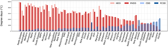
Figure 1. (a) Historical annual HDD and CDD with (darker red and blue) and without (lighter red and blue) population weighting.
Download figure:
Standard image High-resolution imageAn opposite effect is seen in Illinois, Rhode Island, New Jersey, Indiana, Delaware, New Mexico, Arkansas, South Carolina, and Georgia, where more of the population resides in the north. In these states, considering population will slightly increase heating demand and decrease cooling demand, but the differences are limited to 14% and 20%, respectively. When population distribution does not show a notable south-north heterogeneity in the state (see Ohio, Oklahoma, Maryland, and Alabama), incorporating population distribution shows little difference.
Under the business-as-usual scenario, annual heating demand is predicted to decrease while cooling demand is predicted to increase in all states throughout the 21st century, but the magnitude of change varies by state (orange and light green bars in top panel of figure 2). The northern states observe larger reductions in HDD/PHDD and smaller increases in CDD/PCDD than the southern states. In addition to changes in HDD and CDD, population distribution is expected a fundamental shift under the SSP5 scenario (bottom panel of figure 2). The population is projected to increase across most of the U.S., with only minor decreases expected in the West around mountain area. Lager increases are anticipated in the East compared to the West. The most substantial growth is observed in major cities with already high population density, such as New York, Chicago, Los Angles, San Francisco, and Seattle. Such changes are also demonstrated in (Sutradhar et al 2024).
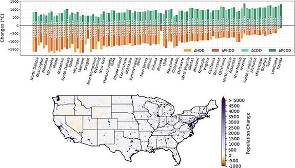
Figure 2. Top panel: future changes in HDD and CDD with (darker orange and green) and without (lighter orange and green) population weighting by the late century. Corresponding changes by mid-century are presented by crosshatched grey bars. Bottom panel: changes in population count from 2010 to 2100 under the SSP5 scenario.
Download figure:
Standard image High-resolution imageChanges in population distribution will result in more growth in cooling demand and a slighter decrease in heating demand in most of the states (top panel of figure 2). For example, in states like Washington, Wyoming, and Organ where population is expected to grow in the north of the state, the absolute value of ΔPHDD is less than that of ΔHDD. This is because the impact of rising temperature (resulting in reduced heating demand in the north) is somehow offset by the population growth (leading to more heating demand). Similar effect is seen in Nevada, but it is due to the decline in its population, particularly in in the north. Given the significant implications of population projection on state-level energy estimation, our subsequent analysis presents how the population-weighted degree days change along with the temperature and population change.
3.2. Evolution of dominant PDD and EDD in the 21st century
3.2.1. Dominant degree-days
Historical and future PHDD and PCDD in each state are compared in figure 3. Historically, 37 out of 48 states in the U.S. have experienced larger annual PHDD than PCDD (henceforth termed as heating-dominant), with the ratio of annual PHDD to PCDD ranging from 2 to 20. This means that these states require at least twice and at most 20 times as much energy for heating compared to cooling purposes. Conversely, in Florida, Arizona, and Louisiana, more energy (up to eight times) is needed annually for cooling than for heating purposes. In Nevada, Texas, Alabama, Arkansas, Mississippi, Georgia, Oklahoma, and South Carolina, PHDD and PCDD are about the same.
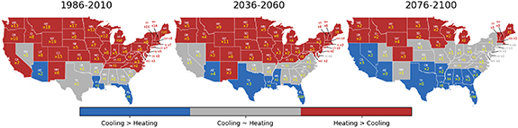
Figure 3. Comparison between heating and cooling in each state for recent past (left), mid-century (center), and late-century (right). Red states: PHDD > PCDD, and the numbers show the factor of PHDD to PCDD. Blue states: PCDD < PHDD, and the numbers are the factor of PCDD to PHDD. Grey states: PCDD ∼ PHDD. The numbers show the factor of either way when they are under 1.5.
Download figure:
Standard image High-resolution imageAs a result of temperature increases and population shift, most middle and southern states are projected to shift their dominant demand from heating to cooling. Consequently, the number of heating dominant states will reduce from 37 (the recent past) to 32 by mid-century and to 16 by late-century. Moreover, the projected trend indicates a heightened cooling-to-heating ratio, potentially even exceeding 35 in Florida by the late-century which is more than four times the current value, 8. These changes suggest that southern states will need a substantially increased amount of electricity to meet the escalating demand for cooling. Meanwhile, in many northern states like New York and Illinois, energy used to meet heating demand, like natural gas and oil might experience a sharp decrease, while a higher allocation of energy (electricity) is expected for cooling purpose. Hence, U.S. grid systems and energy management would confront substantial challenges from this heating-to-cooling transformation.
While the rising temperature is the primary driver for the heating-to-cooling transition in the U.S., changes in population distribution also play undeniable roles. In general, considering population change tends to slow down the heating to cooling shift. A figure equivalent to figure 3, but which solely considers temperature rise, is included in the supplementary materials (figure S.2). By the mid-century, including population change reveals higher heating-to-cooling ratios in the heating dominant states located in the northwest, such as Washington, Wyoming, and Organ. In these states, population projection slows down the reduction of heating while having a minor impact on cooling demand (as discussed in section 3.1), thus it maintains the significant role of heating and leads to a high heating-to-cooling demand ratio. Florida exhibits a higher cooling-to-heating ratio, primarily due to population growth exerting a more substantial impact on the increase of cooling demand than on decrease of heating demand in this state (see figure 2). By the late-century, impacts of population change are mainly reflected on further widening the gap between cooling and heating demands in southern states by accelerating the increase in their cooling demands.
3.2.2. Energy degree-days
State-level annual EDD was calculated by adding annual PHDD and PCDD for an individual state to represent the combined energy demand for heating and cooling (Sivak 2008, Petri and Caldeira 2015). We note that EDD does not represent an equivalent change in primary energy demand (Mima and Criqui 2015) since it does not consider differences between the heating and cooling energy, such as cost and efficiency. As such, we present EDD as a climate-relevant indicator for total energy demand.
As the climate warms, annual EDD is predicted to decrease in northern states and increase in southern states throughout the 21st century (figure 4 left). Decreases in annual EDD in northern states are attributed to the larger reduction in PHDD than the increase in PCDD (see figure 2). Maine and Vermont see the largest decreases in annual EDD because these states concurrently experience the most significant PHDD decreases alongside the smallest PCDD increases. Likewise, due to the small PHDD decreases and large PCDD increases, the fastest EDD increases are noted in Florida, Louisiana, Texas, and Arizona.
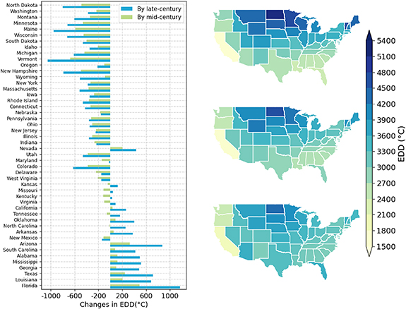
Figure 4. Left: changes in the EDD by mid-century (green) and by late-century (blue). Right: state-level EDD over the eastern U.S. for the recent past (upper right), mid-century (center right), and late-century (lower right).
Download figure:
Standard image High-resolution imageIn northern states, the first half of the 21st century is projected to see greater decreases in EDD than the second half of the 21st century. In contrast, southern states are projected to see larger increases in EDD during the second half of the 21st century. The main reason for this difference is that decreases in PHDD are relatively consistent throughout the 21st century, while increases in PCDD are projected to be larger in the second half of the 21st century. In mid-continent states (from Kansas to Tennessee, except California in figure 4), annual EDD is expected to decrease by mid-century but to increase by late-century, relative to the recent past. This phenomenon can also be attributed to the pace of changes in PHDD and PCDD over the course of the 21st century.
As a result of these changes, the pattern of EDD over the U.S., especially the eastern U.S., is expected to become more homogenous (figure 4 right). During 1986–2010 (figure 4, upper right), annual EDD in the northern states significantly surpassed that in the southern and western states, with the maximum EDD (5168 °C in North Dakota) being over three times higher than the minimum EDD (1604 °C in California). As EDD decrease in the north and increase in the south, the ratio of the maximum and minimum EDD will diminish from 3.2 to 2.3 by the late-century, leading to a more uniform EDD pattern across the U.S. In the eastern part, Georgia will replace Florida and become the state with the lowest energy demand.
3.3. Analysis of monthly PHDD, PCDD, and EDD
Monthly PHDD and PCDD for each state for the recent past, mid-century, and late-century are provided in the Supplementary Materials. In the recent past, the maximum PHDD has occurred in December and January in all states, while the maximum PCDD has been seen in July and August. This peak pattern will remain the same throughout the 21st century. The most noticeable declines in PHDD are expected during the winter months of December and January, whereas the most substantial increases in PCDD are projected from July and August within northern states to September and October within southern states.
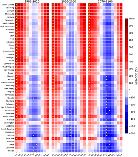
Anticipated shifts in monthly PHDD and PCDD are poised to facilitate a transition from heating dominance to cooling dominance during the spring and fall months, thereby extending the cooling season. As a result, the length of the cooling season is projected to increase by 1 month by mid-century and by 2 months by the late-century. The historical duration of the cooling season suggests four groups for characterizing future cooling season changes. Here, we use the order of the states presented in figure 5 for discussion with a focus on transformations projected by the late-century.
Figure 5. Comparison between monthly HDD and CDD in each state for the recent past, mid-century, and late-century. Red: HDD outweighs CDD in the given month (heating season); blue: CDD outweighs HDD in the given month (cooling season); yellow star: the month when maximum EDD occurs.
Download figure:
Standard image High-resolution image
In the first group (from North Dakota to Utah, as well as Maine and Oregon), cooling seasons will expand from a duration of 2 to 3 months to a span of 4 months, with the addition of June and September as new cooling months. In the second group, encompassing Iowa to New Mexico plus Massachusetts, New Jersey, Rhode Island, and New York, the cooling seasons are poised to extend from 4 to 6 months, marked by the transformation of May and October into cooling months. In the third group, including states from Missouri to California, the present cooling seasons (May–September) are projected to commence in April and persist until October by the conclusion of the 21st century. In the remaining group, cooling seasons are poised to envelop the spring and fall months in Texas and Louisiana while encompassing the entirety of the month in Florida.
Changes in EDD also vary from month to month and across states (monthly EDD is presented in supplementary materials). Generally, cold winter months see negative EDD changes, and hot summer months see positive EDD changes. Monthly EDD shifts within northern states are primarily driven by the reduction in PHDD, whereas in the southern states, these shifts predominantly arise from the increase in PCDD. Meanwhile, in intermediary states, the combined impact of PHDD and PCDD is responsible for the observed changes in monthly EDD.
As EDD increases in some months and states and decreases in others, some states are expected to experience their peak total demand in different months. In figure 5, the month with the maximum EDD in each state is marked by the yellow star. Historically, the highest EDD occurred in winter (January) in most states except Nevada, Arizona, Texas, Louisiana, and Florida (July or August). By mid-century, 7 more states, including Oklahoma, Arkansas, Georgia, Alabama, South Carolina, Mississippi, and California, would have their peak total demand in summer (July or August). By late-century, 20 out of 48 states will see their peak total demand in summer, mainly in July. In summary, under the business-as-usual scenario, many states in the eastern U.S. will see their highest monthly demand in summer instead of winter. Such changes would pose challenges to local energy planning and production, given that the energy demand in different seasons is fulfilled by different fuels.
4. Conclusion
4.1. Main findings
This study evaluates the future changes in annual and monthly population-weighted degree-days over the 48 states in the contiguous U.S. A multi-model downscaled climate projection (NEX-GDDP) was used to calculate HDD and CDD for the recent past (1986–2010), mid-century (2036–2060), and late-century (2076–2100) under the business-as-usual scenario (RCP 8.5). Then, population weighting was added using NASA's SEDAC population count of 2010, 2050, and 2090 to compute PHDD and PCDD, then EDD (sum of HDD and CDD). In comparison to previous studies (table 1) that have focused on changes in annual HDD and CDD, we provide a more comprehensive analysis by presenting future changes in annual and monthly PHDD and PCDD in individual states and on both annual and monthly scales, we investigate the changes in a single type of demand over time and their respective dominance within the same framework.
We find that accounting for population distribution and its change will lead to a smaller decrease in heating demand and more increase in cooling demand in most states. This result aligns partially with the global-scale analysis conducted by (Kennard et al 2022), where they find that adding population weighting leads to more increase in CDD. However, they found an opposite impact on HDD, adding population weighting leads to more HDD decrease. Such differences can be attributed to the changes in population distribution over the study domains. Analysis of population-weighted degree days shows a more significant PCDD increase in the southern states and a larger PHDD decrease in the northern states. As a result, building energy demand driven by climate and population change in the U.S. will shift from heating to cooling, with the number of cooling-dominant states rising from 3 (out of 48) to 12 by the late-century. Uneven changes in PHDD and PCDD are expected to yield diminished EDD in northern states and increased EDD in southern states, and lead to a more homogenous distribution of total energy demand across the country. Such trend and pattern are also seen in a degree-days analysis by (Petri and Caldeira 2015). With PHDD diminishing and PCDD increasing throughout the year, the duration of cooling seasons will extend by 1 month by mid-century and by 2 months by the late-century in all states. An extended summer is also projected in the Northern Hemisphere by 2100 under the business-as-usual scenario (Wang et al 2021), due to an earlier onset of spring and summer and a delayed onset of autumn and winter. EDD is projected to decline in the winter and increase in summer, leading to the migration of the EDD peak from winter to summer in 14 out of the 48 states.
4.2. Limitations
Using population weighted degree-days as a metric for energy demand has limitations. Although temperature is known to dominate energy use in buildings (Suckling and Stackhouse 1983, Zhai and Helman 2019), other climate variabilities like humidity and solar, can also bring notable impacts (Shen 2017, Li et al 2021). Our measures also do not consider the impacts of non-climate factors like building characteristics, occupancy patterns and behavior, and other socio-economic changes, which play an important role in actual building energy demand (Berrill et al 2021, Mastrucci et al 2021). In addition, using a fixed base temperature for heating and cooling for the entire eastern U.S. may not accurately reflect the threshold for needing heating or cooling in some locations (Huang and Gurney 2016). On the other hand, although we considered population distribution and its future changes, impacts of population concentration in urban agglomerations, such as urban heat island, are not included here. Still, population weighted degree-days are appropriate in this study as the study focuses on changes in energy demand driven by climate and population change, and aims to present changes in larger-scale energy demand shifts rather than changes in building-scale or specific location energy demand.
4.3. Implications
Temperature and population are found to have dominant impacts on changes in large-scale energy demand in the U.S. (Rastogi et al 2019). Our study, incorporating the two main drivers, provides a big picture on future changes in heating and cooling demand across the U.S.
In the U.S., space heating is provided by various sources including natural gas, oil, electricity and/or others (Li et al 2012, EIA 2019); and heating equipment choices differ by region (EIA 2015b). Prominent decreases in heating demand in the northern U.S., as indicated by changes in PHDD, may lead to large reductions in natural gas and oil consumption in these states, and a heating decrease in the south will reduce winter electricity use in southern states. In some northern and middle states, lower heating demand may provide great potential for switching heating sources from natural gas to electricity, and large central furnaces may be replaced by heat pumps or electric portable heaters. What's more, significantly lower heating demand in northern states may also reduce the efficiency of heating systems installed at early construction stages, which can lead to higher costs and energy consumption (Riise and Sørensen 2013, Sekhar et al 2018) and lower thermal comfort (Sekhar et al 2018).
Space cooling in the entire U.S. is largely met by electricity (Dell et al 2014, Zhou et al 2014). More intense and prolonged cooling seasons, as indicated by changes in PCDD, can challenge local utilities to provide more electricity (Zhai and Helman 2019). Spikes in demand in southern states and summer months when cooling demand is already the largest can create additional stress on electricity transmission and distribution systems (Denholm et al 2012). Fast-growing cooling demand can also challenge current cooling systems whose capacity is designed for the historical climate (ASHRAE 2013).
Since electricity may be generated from a wide range of sources, including fossil fuels like coal and natural gas to renewable energy like wind and solar at the state level or even smaller utility-scale levels (EIA 2022), changes in electricity demand due to higher building cooling needs in each state can inform energy planning. The shift of demand from heating to cooling in the eastern U.S. would require additional electricity, affecting the power allocation in the U.S. power systems.
In a large, geographically diverse nation like the U.S. where each state has different regulations and characteristics (Auffhammer and Mansur 2015), conducting state-level analysis is particularly important. While actual energy demand will also depend on building structures, building use, and heating and cooling technologies, our results still provide a valuable insight into sectors such as utilities, fuel companies, and HVAC (Heating, Ventilation, and Air Conditioning) companies, as well as fuel consumption and energy planning, and support energy conservation and climate adaptation at the state level as well as the national level.
Acknowledgments
We acknowledge financial support from the Office of Sustainability at the University of Wisconsin-Madison (UW-Madison). We would also like to express our thanks to Dr Missy Nergard from the Office of Sustainability at the UW-Madison for their valuable suggestions, Dr Doug Ahl at the Slipstream for helpful discussions, and to the Coupled Model Intercomparison Project (CMIP) participants for producing and making available their model output.
Data availability statement
All data that support the findings of this study are included within the article (and any supplementary files).
Conflict of interest
The authors declare that they have no known competing financial interests or personal relationships that could have appeared to influence.
Supplementary data (1.1 MB DOCX)