

Abstract
The development of a high-quality wildfire occurrence model is an essential component in mapping present wildfire risk, and in projecting future wildfire dynamics with climate and land-use change. Here, we develop a new model for predicting the daily probability of wildfire occurrence at 0.1° (∼10 km) spatial resolution by adapting a generalised linear modelling (GLM) approach to include improvements to the variable selection procedure, identification of the range over which specific predictors are influential, and the minimisation of compression, applied in an ensemble of model runs. We develop and test the model using data from the contiguous United States. The ensemble performed well in predicting the mean geospatial patterns of fire occurrence, the interannual variability in the number of fires, and the regional variation in the seasonal cycle of wildfire. Model runs gave an area under the receiver operating characteristic curve (AUC) of 0.85–0.88, indicating good predictive power. The ensemble of runs provides insight into the key predictors for wildfire occurrence in the contiguous United States. The methodology, though developed for the United States, is globally implementable.
Export citation and abstract BibTeX RIS

Original content from this work may be used under the terms of the Creative Commons Attribution 4.0 license. Any further distribution of this work must maintain attribution to the author(s) and the title of the work, journal citation and DOI.
1. Introduction
Wildfire poses a significant risk to both the natural environment and people. Wildfires are increasing in many parts of the world, including the United States, the northern boreal zone, southern Europe, Amazonia, and Australia (Smith et al 2020) in response to ongoing climate change, which has been associated with a strong drying effect on vegetation fuels (Ellis et al 2022). Wildfire is also an important earth system process. In addition to the effects of radiative forcing and carbon emissions on climate (Liu et al 2014), wildfire has been found to influence Amazon regrowth after deforestation (Drüke et al 2023), to be a major driver of permafrost thaw (Gibson et al 2018); and to cause significant ocean fertilisation events (Weis et al 2022). It is thus critical to be able to make quick and robust predictions of the likelihood of wildfire events, both to characterise wildfire risk and to better understand wildfire's complex role in the earth system.
Wildfire occurrence can be defined as the development of an unplanned fire over a certain size. Occurrence, in conjunction with fire size, controls annual burned area—the cumulative footprint of wildfire on the landscape. The rate of wildfire occurrence is related to fire intensity (Luo et al 2017), a key determinant for the severity of a burn event. The likelihood of fire occurrence is the first component in process-based fire models used in dynamic global vegetation models (Rabin et al 2017). Wildfire occurrence is also of importance from a fire management perspective because of the need to identify and control smaller wildfire events in high-risk areas.
Wildfire occurrence is driven by many factors, reflecting the multiple conditions that must be met for ignition and initial fire spread: an ignition source, fuel availability, fuel dryness, and atmospheric conditions (Krawchuk et al 2009, Harrison et al 2010). Ignitions may be caused by lightning or humans, but there are many human sources of ignitions including recreation, smoking, debris burning, arson, machinery, railroads and powerlines (Short 2014). However, humans also suppress wildfires, either directly through fuel management and firefighting, or indirectly through the impacts of land-use and landscape fragmentation on fuel availability and continuity (Harrison et al 2021). Fuel accumulation is also determined by vegetation characteristics, including primary production and dominant plant type (Harrison et al 2010, Forkel et al 2019). Meteorological drivers such as precipitation, atmospheric moisture, and temperature influence fire occurrence through their effect on fuel moisture, while topography and wind strength influence the rate of spread (Parisien and Moritz 2009). In addition to current conditions, antecedent vegetation growth and drought also influence the occurrence of wildfires through their effect on fuel availability (Kuhn-Régnier et al 2021). Given the large number of potential influences on wildfire occurrence, it is important to consider which are most important in order to define a parsimonious set of predictors to incorporate into a wildfire occurrence model.
The probability of wildfire occurrence is primarily modelled as a monthly to decadal landscape susceptibility to wildfire. Highly resolved, regional fire susceptibility maps account for local effects driving fire likelihood in different regions based on either statistical models, machine-learning or maximum entropy approaches (D'Este et al 2020, Gholamnia et al 2020, Chen et al 2021). Daily timescale variability in the probability of wildfire occurrence is often accounted for using fire danger rating systems, risk indices that are largely based on modelling meteorological effects, with some limited integration of remote sensing and fuel mapping products (Zacharakis and Tsihrintzis 2023).
In this paper we introduce an adapted Generalised Linear Model (GLM) methodology to model the daily probability of wildfire. GLMs are statistical models that establish the most likely linear relationship between a dependent variable and a set of predictors, taking into account the statistical properties of the dependent variable. The approach was adopted here because it provides more easily interpretable results than machine learning or non-linear statistical methods and is also less susceptible to overfitting, which is important given the highly stochastic nature of wildfire occurrence. We then apply this in an ensemble of models to determine the spread of model performance, and to identify which predictors are most essential to modelling the likelihood of daily fire occurrence. We evaluate the model's performance across geospatial and seasonal trends, and its representation of interannual variability.
2. Methods
2.1. Data
2.1.1. Fire occurrence data
The target fire occurrence variable was developed from the fire programme analysis fire-occurrence database (FPA FOD) (Short 2021), a synthesis of wildfire occurrence across the United States from data provided by federal, state and local fire organisations covering the period 1992–2018. Prescribed burns are not included in the dataset, but escaped fires that result from prescribed burns are included. The fire start location is given to a resolution of 1.6 km. We use data from 2002 onwards because the quality of non-federal reporting systems is better after this date (Short 2014). We define a fire occurrence as an unplanned fire greater than 0.25 acres (0.1 ha)—the lowest non-zero U.S. National Wildfire Coordinating Group fire size classification. The binary data (occurrence, non-occurrence) were gridded at daily, 0.1° resolution.
2.1.2. Predictors
A total of 47 predictors representing meteorological, vegetation and human factors affecting the probability of fire occurrence were used (supplementary table A1). Precipitation and temperature-related variables were obtained from the PRISM Climate Group (2019), with additional meteorological variables taken from ERA5-Land (Muñoz-Sabater et al 2021). These data were used to derive predictors (e.g. antecedent precipitation) associated with antecedent conditions over several different time periods. Convective available potential energy data, a predictor of lightning occurrence, was sourced from the National Centres for Environmental Prediction's North American Regional Reanalysis (NCEP-NAAR: Mesinger et al 2006). Rural and total population density were obtained from version 4 of the Global Population of the World dataset (CIESIN 2016). Road density was obtained from version 4 of the Global Roads Inventory Project data set (Meijer et al 2018) and additional measures of human activity (e.g. powerline length per area) from OpenStreetMap (OSM Contributors 2022). The land-cover fraction of different vegetation types (e.g. herbaceous cover) was obtained from the European Space Agency Climate Change Initiative data set (Defourny et al 2019). Gross primary production (GPP) was derived using a light-use efficiency model (P model: Stocker et al 2020) driven by the remotely-sensed fraction of absorbed photosynthetically active radiation (Jiang and Ryu 2016), photosynthetic photon flux density (Ryu et al 2018) and climate data. Antecedent effects on fuel accumulation, fuel drying and fuel wetting, represented by antecedent GPP, vapour pressure deficit (VPD) and precipitation respectively, were included through testing different timescales for each predictor through test runs of the model at varying antecedences. All the predictor variables were re-gridded to 0.1° resolution and linearly interpolated to a daily timescale.
2.2. Modelling approach
We used a binomial GLM to model the binary outcome of whether a wildfire greater than 0.25 acres occurred on a given day at a given location. GLMs provide highly interpretable results distinguishing the effect of each predictor when other predictors are held constant (Nelder and Wedderburn 1972) and provide a measure of variable significance in the form of t-values (McCullagh and Nelder 1989). There are well-established frameworks for evaluation of model performance and predictors, including the Akaike information criterion (AIC) (Akaike 1974) and the variance inflation factor (VIF) (Allison 1999) used in this study. We used the area under the receiver operating characteristic curve (AUC) as an overall performance metric. GLMs have been widely applied to model wildfire, both in a global context (e.g. Bistinas et al 2014, Haas et al 2022), and in regional fire occurrence modelling (e.g. Vilar et al 2010, Lan et al 2023).
We developed our new model in Python, using the statsmodels module. The standard bionomial approach was modified in three ways for this application (figure 1). We introduced an objective predictor selection procedure, given the large number of potential predictors (table A1), in order to minimise multicollinearity in the predictors and overfitting the model. A stepwise variable selection algorithm (Chowdhury and Turin 2020) was applied, starting from a constant model with no predictors and then iteratively (1) finding the best performing new variable to add by minimising the AIC (the forwards step), before (2) checking whether removing any of the existing predictors for an unused variable minimises the AIC further (the backwards step). Predictor variables that produced VIFs >5 were ignored in both steps, to prevent inclusion of highly correlated predictors. Improvements in predictivity (AUC) were negligible after 12 predictors; this was therefore taken as the maximum number of predictors to reduce the likelihood of overfitting.
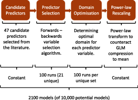
Figure 1. An overview of the GLM architecture and the ensemble application of the modelling methodology. The inputs and adaptations to a basic GLM application are detailed in the top two layers, with the second two layers showing 100 predictor selection runs, and subsequent 100 runs of the predictor domain optimisation algorithm.
Download figure:
Standard image High-resolution imagePredictors may only influence fire occurrence probability in a certain range. For example, small increments in daily precipitation are more likely to impact fire occurrence probability when the precipitation rate is low. Predictors may also have different effects on the probability of fire in different parts of their range. Aridity, for example, lowers fuel moisture and leads to higher fire risk, but further increases in aridity leads to less vegetation growth, decreasing fuel availability and fuel continuity and hence leading to lower fire risk. We determined the appropriate range of influence for each predictor through an algorithm that truncated the predictor ranges through optimisation of the AIC. The algorithm (given in supplementary material, figure A1) iteratively tested the improvement of the model by clipping the upper or lower bound of each predictor. The final set of predictor domains is defined as the set of upper and lower bounds on each predictor from which there is no further significant improvement in AIC—with an AIC difference of two taken as a substantial difference in models (Burnham and Anderson (2004)).
GLMs have a known tendency to compress predicted values towards the middle of the sampled range and to under-represent high and low extremes (Hastie et al 2009) due to the assumption of linearity with the log odds of the target variable. Whilst a good ranking of high and low fire risk was achieved in the model (i.e. high AUC), compression was observed in the geospatial mean of the probability of fire occurrence between 2002–2018. We applied a power-law transformation to the output daily probability of fire occurrence, optimising to reduce the residuals in the distribution of the observed and modelled geospatial means.
2.3. Ensemble application of model
We created an ensemble of models by running the predictor selection algorithm 100 times with a training dataset of 107 datapoints and running the predictor range optimisation algorithm 100 times for each unique set of selected predictors with a training dataset of 106 datapoints. This produced an ensemble of 2100 members. This ensemble allows us to characterise the spread of model performance and to evaluate whether the model performs well given the uncertainties introduced by variable selection and range optimisation. We use the mean of the Pareto superior subset (Jahan et al 2016) of the ensemble, which is less likely to be overfit than a single 'best performing' ensemble member, to represent fire probability. The Pareto superior subset is defined as the set of all Pareto efficient models across the four model benchmarks defined in section 2.4. An additional 2000-member ensemble was created by running the predictor selection algorithm with a training dataset of 106 datapoints to identify the rate at which each of the candidate predictor variables was selected. The higher number of runs was required due to the low rate of selection for some variables and to better assess whether some core variables were always selected, the smaller training dataset was a necessary cost due to the relatively higher number of runs.
2.4. Evaluation metrics
We used the AUC statistic to assess predictive power through separability—the extent to which the model can separate between wildfire occurrence and non-occurrence (Hanley and McNeil 1982). The normalised mean error (NME) between the modelled and observed mean rate of wildfire occurrence for each cell over the study period of 2002–2018 was used to assess performance with respect to geospatial trends. The NME of the total number of wildfire occurrences was used to assess the representation of interannual variability. Seasonal effects were evaluated in terms of seasonal concentration and seasonal phase (Hantson et al 2020). Seasonal concentration is the extent to which fire occurrence is clustered in the year, where 0 indicates that there are the same number of fires each month and 1 indicates fires occur in a single month; this was assessed using NME. Seasonal phase is the peak timing the fire season, and is most meaningful when the season is characterised by a single, symmetrical peak. Seasonal phase was assessed using the mean phase difference (MPD) (Hantson et al 2020). NME and MPD were calculated as follows:
where Ai are cell areas, ϕ is seasonal phase, and X is either the mean rate of fire occurrence per site, the total annual number of fires, or the seasonal concentration. An NME value of 0 corresponds to perfect performance, whilst a value of 1 means performance equal to a null model predicting a constant value of X for all datapoints. An MPD of 0 means the model and observation are in perfect phase, whilst a value of 1 would mean perfect antiphase.
3. Results
The overall performance of the model as measured by the AUC is good (table 1). All the models have an AUC of >0.85, higher than the threshold of 0.8 generally taken as indicating 'very good' model performance (McCune et al 2002). The Pareto subset of models have an AUC of >0.86.
Table 1. AUC and benchmark metrics for all ensemble members, the Pareto superior subset and the highest AUC model of the Pareto superior subset (the 'best model').
| All ensemble members | Pareto superior subset | Best Model | |||||
|---|---|---|---|---|---|---|---|
| Min | Mean | Max | Min | Mean | Max | ||
| Separability (AUC) | 0.85 | 0.87 | 0.87 | 0.86 | 0.87 | 0.87 | 0.87 |
| Geospatial (NME) | 0.43 | 0.45 | 0.49 | 0.43 | 0.44 | 0.46 | 0.44 |
| Annual fire count (NME) | 0.66 | 0.67 | 0.68 | 0.66 | 0.67 | 0.67 | 0.67 |
| Seasonal concentration (NME) | 0.70 | 0.83 | 1.02 | 0.70 | 0.78 | 0.88 | 0.74 |
| Seasonal phase (MPD) | 0.13 | 0.15 | 0.17 | 0.13 | 0.14 | 0.16 | 0.15 |
The model has a geospatial NME for the Pareto subset of the ensemble of 0.44, considerably better than a null model assuming the mean value of fire probability across all cells. The poorest NME score from the full ensemble (0.49) is also very good. The model identifies key features of the geospatial patterns shown by the mean of the model output from 2002 to 2018 (figure 2), such as the broad regions of lower fire likelihood in the Mississippi Valley, the Corn Belt and the Great Plains, and the areas of higher fire likelihood such as the Southeastern and Texas Plains and the West Coast. These patterns are also observed in the daily outputs (see figure A2 for examples). Even at a finer scale, the model generally captures the high and low fire areas within a region. However, the model output is smoother than the observations. The area with <10−4 average daily probability of wildfire occurrence is 37% smaller than for the observations, and the model shows none of the discontinuities at State boundaries seen in the observations, such as those seen at the New York and North Carolina state borders.
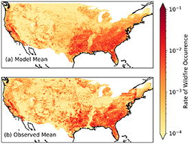
Figure 2. Comparison of (a) modelled and (b) observed mean of daily modelled probability of wildfire occurrence over the period 2002–2018. The model results are the average across the Pareto superior set of ensemble members. Both maps are plotted on a logarithmic scale.
Download figure:
Standard image High-resolution imageAs with the geospatial patterns, the model also produces reasonable spatial patterns for wildfire seasonality (figure 3). The mean MPD value for the Pareto subset of 0.14 for seasonal phase indicates that the phasing of the fire season is well captured. Model performance for seasonal concentration is less good, with a mean NME value for the Pareto subset of 0.78. Nevertheless, the model identifies the early spring phase for wildfire in the southeast, the late spring phase in the northeast, and the late spring/summer phase in the west. It also correctly identifies the less concentrated fire season in the Southeastern and Great Plains, as well as towards the coasts. However, the observations are considerably noisier than the model, particularly in low fire regions. Figures A3–A5 in the supplementary material show the three most observed seasonal patterns, a spring fire season; a spring/autumn bimodal fire season; and a summer fire season respectively.
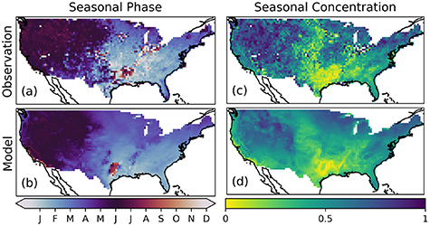
Figure 3. Comparison of (a) observed and (b) modelled seasonal phase and (c) observed and (d) modelled seasonal concentration of wildfire occurrence.
Download figure:
Standard image High-resolution imageThe model is also able to predict high and low fire years (figure 4). The model has an interannual NME for total annual fire counts for the Pareto subset of the ensemble of 0.67, much better than a null model assuming the mean value of fire probability across all years. Figure A6 in the supplementary material contrasts the mean modelled and observed rate of fire in the years with highest (2006) and lowest (2003) number of fire occurrences.

Figure 4. Annual total modelled and observed fire occurrences in the contiguous United States from 2002–2018.
Download figure:
Standard image High-resolution imageAnalysis of the 2000-model ensemble of the predictor selection component of the model (figure 5) shows that several variables are identified as important predictors in all the runs. Rural population density, snow-cover fraction, precipitation over the prior five days, and the diurnal temperature range (DTR) were selected in all 2000 models, and night-time VPD was selected in 98% of the runs. A further seven predictors are selected in more than 50% of the runs: GPP over the antecedent year and over the antecedent 50 d, tree cover fraction, shrub cover fraction, herb cover fraction, aridity and daily precipitation—emphasising the importance of vegetation and moisture controls on wildfire occurrence probability. However, some predictors were rarely or never selected, including ruggedness, soil moisture and measures of human infrastructure.

Figure 5. Rate of selection of individual predictor variables in the 2000-member ensemble from the stepwise variable selection algorithm. Only variables that were selected in more than 1% of the ensemble members are shown.
Download figure:
Standard image High-resolution image
4. Discussion
We have presented a model to predict the daily probability of wildfire occurrence which has good predictive power. All models have an AUC of greater than 0.85, higher than the threshold of 0.8 for 'very good' model performance taken in other studies (McCune et al 2002). Similarly good performance has been obtained with models focusing on more limited regions, for example a daily lightning fire occurrence model for Daxinganling Mountains (AUC = 0.87) (Chen et al 2015), and an hourly forest fire risk index developed for South Korea (AUC = 0.84) (Kang et al 2020). However, both of these studies focus on a relatively short time period (6 years) and more climatologically and ecologically homogeneous regions. Our research shows that reliable predictions of the daily probability of wildfire occurrence can be made using statistical models through careful adaptation of a GLM methodology, and provides a roadmap for how to do so.
Whilst there is good correspondence between the modelled and observed geospatial patterns (figure 2), there are also regions of disagreement. The most marked difference between the modelled and observed mean rate of wildfire occurrence is in the northeast US. This may reflect a problem with the FPA FOD data for fire numbers since there is poor agreement, except for New York state, between these data and annual fire count estimates from the National Interagency Coordination Centre (NICC) (Short 2014). However, despite the poor match in the predicted rate of fire in the northeast and the FPA FOD data, the model still identifies key regional effects, including the greater amount of fire on the New England coast compared to inland, and the comparatively low rate of fire in the upstate New York boreal highlands. The model tends to identify more fire in agriculturally intensive regions such as the corn belt and the Mississippi valley. This may reflect more systematic fuel removal and landscape management in these regions. However, this region includes states where the FPA FOD dataset predicts a lower rate of wildfire than the NICC estimates (Missouri, Indiana and Ohio), so it may be that the FPA FOD dataset is under-reporting wildfire counts in these regions whilst the model is correctly responding to causal factors associated with a higher mean rate of fire occurrence.
We have shown that there is good first-order correspondence between the observed and modelled seasonal concentration and phase of wildfires. The match is less good in low fire regions, where the noisiness of the observational records affects the reliability of the metric. There is also a major disagreement between the modelled and observed seasonality in the Pacific Northwest, where the model incorrectly predicts a late spring peak in wildfires compared to the observed early summer phasing. One potential reason for this mismatch is that evergreen forests are less susceptible to spring wildfires than deciduous forests, since the canopy protects leaf litter from drying out (Tamai 2001). However, this cannot be the only explanation for the poor model performance in the Pacific Northwest because the wildfire seasonality in other regions where evergreen forests are dominant is predicted reasonably well. The largest mismatches between the predicted and observed timing of fire peak occur in grid cells with extremely high annual precipitation, with values >99.5th percentile in the overall data set. It is to be expected that the model has more difficulty in capturing extremes that are poorly represented in the training data but it is clear that the power-law transformation used to minimise the impact of outliers has not overcome this limitation completely.
The ensemble of 2000 predictor selection runs showed that rural population density is an important predictor in all models whereas total population density is not. Total population density has been used as a predictor of wildfires both in global statistical models (e.g. Bistinas et al 2014, Haas et al 2022) and in fire-enabled dynamic global vegetation models (Rabin et al 2017). Despite the fact that Fusco et al (2016) discounted population density as a meaningful predictor at local scales in the U.S. compared to land-use predictors, our study shows that rural population density is an informative metric. Specifically, increases in rural population lead to an increased probability of fire occurrence. This is consistent with the findings of Balch et al (2017) that human ignitions occur on days and in regions that are wetter than those under which fires start naturally, thus creating an expansion of the 'fire niche'.
The ensemble of predictor selection runs emphasises the importance of meteorological variables in controlling fire occurrence. Both night-time VPD and DTR were identified as important predictors, reflecting the different effects on daily fluctuations in fuel moisture from the dampening effect of the antecedent night-time moisture barrier (Goens 1989) and the drying effect from warming throughout the day. GPP was found to be an important control on wildfire occurrence at both annual and seasonal antecedences—reflecting the effects of consequently higher fuel load and live fuel moisture respectively. This supports the conclusions of Kuhn-Régnier et al (2021) that including antecedent conditions for vegetation predictors produces more accurate predictions of burnt area.
There are several potential applications of the model and modelling approach described here. The probability of fire occurrence over the short-term at a regional scale for the purposes of fire and landscape management is usually predicted using fire index models which rely on detailed fuel catalogues and drying models (e.g. Preisler et al 2014). Similar predictions can be made with our model even in the absence of detailed fuel load information. Furthermore, the model could be applied to predict likely future changes in wildfire occurrence using ensembles of climate model projections and without assuming static (modern observed) fuel loads. Near term prediction of the occurrence of fires over a given size would be useful to stakeholders exposed to wildfire risk, including the insurance sector and land managers. Although our model was originally developed for the contiguous United States, because of the availability of high-quality data particularly on variables related to potential human influences on wildfires, the final set of selected variables are obtainable from readily available global data sets. Thus, the same modelling approach could be employed to assess fire risks in other regions and how these might change with a changing climate. It would be interesting to compare different regions of the world to determine how the key drivers of wildfire vary regionally, as has been suggested by several previous studies (e.g. Bistinas et al 2014, Forkel et al 2019). The model may also have utility in the context of fire-enabled dynamic vegetation models. The current generation of fire-enabled dynamic vegetation models do not predict the seasonality or interannual variability of wildfires well (Hantson et al 2020). This is a major limitation given that these models are now included in earth system models used to predict future climate changes in order to simulate the feedback associated with fire emissions (Park et al 2023, Wang et al 2023). Our modelling approach could be used to provide a way of realistically predicting fire starts, replacing the simplistic ignition assumptions currently based on lightning strikes or a human population density, that could then be coupled to the process-based fire spread component of the global fire models.
5. Conclusion
We have presented a new model to predict the probability of wildfire occurrence that produces realistic predictions at a daily timescale and 0.1° resolution for the contiguous United States. It captures the geographic differences both in the numbers and the seasonal occurrence of fires, as well as predicting high and low fire years. The most important predictors of the probability of wildfire occurrence are rural population, meteorological variables (short-term drying, precipitation and snow cover) and vegetation properties (plant type cover and antecedent GPP). The model is easily applicable and, given that all the variables are available in global data sets, could be applied to predict fire risk worldwide under a changing climate.
Acknowledgments
We thank Hannah Cloke for suggestions about the ensemble approach, Wenjia Cai for assistance with the P model. We also thank Ted Shepherd, colleagues from AXA-XL Ioana Dima-West and Alec Vessey, and colleagues at the Leverhulme Centre for Wildfires, Environment and Society for discussions of the results. This work is a contribution to the LEMONTREE (Land Ecosystem Models based On New Theory, obseRvations and ExperimEnts) project, funded through the generosity of Eric and Wendy Schmidt by recommendation of the Schmidt Futures program (T R K, S P H, I C P). T R K also acknowledges support from the SCENARIO NERC Doctoral Training Programme (NE/S007261/1). I C P also acknowledges support from the ERC-funded project REALM (Re-inventing Ecosystem And Land-surface Models, Grant No. 787203).
Data availability statement
All of the data sets used in the analysis are publicly available from the references cited in table A1. The outputs of the model and the code are available from https://zenodo.org/record/8392712.
The data that support the findings of this study are openly available at the following URL/DOI: https://doi.org/10.5281/zenodo.8392712.
Author contributions
Concepts, strategy and interpretation were developed by T R K, S P H and I C P jointly. T R K was responsible for data curation, processing and analysis, and produced the graphics and tables. T R K wrote the original draft and all authors contributed to the final version.
Conflict of interest
The authors declare that they have no conflict of interest.
Supplementary data (1.8 MB PDF)