

Abstract
We objectively analyzed historic radar reflectivity images and diagnosed mature mesoscale convective systems (MCSs) in South China during the spring season (March to May) of 2009–2019. Our goal was to understand the climatological features of mature MCSs, their interannual variations, and potential connections with surface aerosol pollution. Springtime MCSs over South China were most frequently observed in the central and east-coastal parts of Guangdong Province. The mean monthly half-hourly counts of MCSs over South China in March, April, and May were 103 ± 83, 274 ± 298, and 337 ± 225, respectively, with considerable variability from year to year. Approximately 89% of springtime MCSs over South China had a linear or quasi-linear structure, with convective precipitation covering on average 34% of the total precipitating area of each individual MCS, anmied 63% of MCSs consisted of a stratiform precipitation area trailing the convective precipitation. In March, MCSs occurred most frequently mid-day; in April and May, MCSs were most frequent around midnight. From 2013 to 2019, the MCS occurrences in April were significantly lower during years with more aerosol pollution days. This finding potentially supported our previous model study's finding that elevated anthropogenic aerosol levels may suppress April MCS occurrences in South China via aerosol-cloud-radiation interactions. Further research is required to better understand the intricate relationship between aerosol abundance and MCS activities in this region.
Plain Language Summary
Mesoscale convective systems (MCSs) are the main cause of heavy precipitation and weather disasters over South China in spring. We objectively analyzed historic radar images and diagnosed the climatological features of springtime mature MCSs over South China. Springtime MCSs over South China occurred most frequently over central and east-coastal Guangdong and typically exhibited a linear or quasi-linear shape. The occurrences of MCSs varied considerably from year to year. We found that the MCS occurrences in April were lower during years with more aerosol pollution days This finding potentially supported our previous model study that high levels of anthropogenic aerosols suppress MCS occurrences in South China in April.
Export citation and abstract BibTeX RIS

Original content from this work may be used under the terms of the Creative Commons Attribution 4.0 license. Any further distribution of this work must maintain attribution to the author(s) and the title of the work, journal citation and DOI.
1. Introduction
Mesoscale convective systems (MCSs) are highly organized systems of convective precipitation, with spatial scales of ⩾100 km during their mature stage and lifetimes ranging from a few hours to a day (Markowski and Richardson 2010, Houze 2018). MCSs often give rise to high-impact weather that endanger public safety and livelihood, including heavy rain, lightning, destructive winds, and tornadoes (e.g. Ashley and Mote 2005, Zhang et al 2019, Surowiecki and Taszarek 2020). In particular, over South China during the pre-summer rainy season, MCSs are the main cause of heavy rain and contribute approximately 90% of the total precipitation (Luo et al 2020b). Therefore, it is imperative to gain a comprehensive understanding of the spatiotemporal occurrences, morphologies (spatial patterns of precipitation), movements, associations with synoptic weather, and interannual variability of springtime MCSs over South China. Such understanding is vital for accurate weather forecasting, effective disaster management, and informed infrastructure planning.
Several studies have characterized the features of MCSs in different regions of the world by analyzing high-resolution observations indicative of strong convection, such as low cloud-top temperature (e.g. Fiolleau and Roca 2013, Ai et al 2016, Chen et al 2019, Cheeks et al 2020), heavy surface precipitation (e.g. Houze 2004, Prein et al 2017), and strong radar reflectivity (e.g. Houze et al 1989, Haberlie and Ashley 2019, Surowiecki and Taszarek 2020). Over China, the first of such analyses was that of Zheng et al (2013), who manually parsed the radar mosaic reflectivity images over central East China during June to September of 2007–2010 and subjectively classified 47 MCS cases into seven characteristic morphologies. Each of those seven morphologies was distinct in shape, extent, and juxtaposition of convective and stratiform precipitation areas. Similarly, Meng et al (2013), He et al (2016), and Chen et al (2022) manually analyzed radar mosaic reflectivity data over East or South China for a period of 2–5 years and subjectively identified MCSs (or squall lines, a linear subset of MCSs) and their characteristic features. Li et al (2020) analyzed a merged rain gauge-satellite hourly precipitation dataset over East China during 1st May to 15th July of 2008–2016 and identified MSCs as intense, mesoscale precipitating areas of long duration (⩾6.0 h). These analyses concluded that, over South China, MCSs contributed most substantially to monthly precipitation in April and May (Meng et al 2013, Li et al 2020). Springtime MCSs over South China occurred most frequently in the northern parts of Guangxi and Guangdong provinces, propagated eastward, and their precipitation were strongest in early morning (2:00–10:00 local time) with a secondary peak in late afternoon (18:00 LT) (Meng et al 2013, Li et al 2020, Chen et al 2022). Occurrences of springtime MCSs over South China were associated with low-level southwesterly jets and wind shear and positive anomalies of convective available potential energy (Meng et al 2013, Chen et al 2022), consistent with current theories on MCS trigger mechanisms (Houze 2004).
To date, most analyses on Chinese MCSs' features were based on manually and subjectively selected cases and only for a few years. There has been a notable absence of objective studies investigating the long-term climatological features of Chinese MCSs and their interannual variability. MCSs are likely influenced by interannual variations of regional atmospheric circulation, thermodynamic conditions, and the chemical environment, including factors such as the East Asian monsoon, the West Pacific Subtropical High, the low-level southerly transport of moisture, and surface aerosol pollution (Jiang et al 2017, Guo et al 2018, Zhang et al 2020, Luo et al 2020a). Aerosols, in particular, can have diverse impacts on MCSs through complex microphysical, radiative, and thermodynamic processes (e.g. Rosenfeld et al 2008, Fan et al 2016). Previous studies over South China found that increased aerosols would enhance the convection within individual MCSs but would not significantly affect the precipitation reaching the surface (e.g. Jiang et al 2017, Guo et al 2018). However, elevated levels of anthropogenic aerosol may stabilize the surface atmosphere through direct and indirect radiative cooling, thereby suppressing the occurrences of springtime MCSs over South China (Zhang et al 2020). A systematic investigation of MCS's interannual variability over South China may provide insights into on how those MCSs have responded to regional anthropogenic aerosol pollution and the decline of that pollution since 2013 (Jiang et al 2020).
The goal of this study was to characterized the features of mature springtime MCSs over South China and examine their interannual variability from 2009 to 2019. The China New Generation Weather Radar Observation Network (CINRAD), operated by the China Meteorological Administration (CMA), has been observing high-resolution (∼1 km) radar reflectivity since 1999. However, native radar observations and historical radar reflectivity data are not publicly available in China, which poses a challenge for systematically investigating MCS characteristics and their interannual variability. To overcome this challenge, we developed an objective diagnostic algorithm of mature MCSs using publicly available historic radar mosaic reflectivity images (section 2). We analyzed the characteristics and interannual variability of mature MCSs and investigated the potential connections between surface aerosols and MCSs in this region (sections 3 and 4).
2. Data and methods
2.1. Radar reflectivity observations and surface particulate matter measurements over South China
We analyzed historic mosaic images of radar reflectivity from CINRAD over South China during spring (March–May) from 2009 to 2019. Figure 1(a) shows the locations of the 49 S-band radar stations and their scanning areas. The CMA created mosaic radar reflectivity images by combining the lowest three elevation angle (0.58°, 1.58°, and 2.48°) scans from each individual radar and by applying preliminary quality control procedures (e.g. removal of systematic deviations between radars, removal of ground clutter signals, range-aliasing, and correction of radial velocity) (Xiao and Liu 2006). The radar reflectivity was color-coded in 5 dBZ intervals. The mosaic images were saved as single-layer GIF or PNG files with a pixel resolution of approximately 2.1 km (figures 1(b) and (c)). We trimmed all images to a consistent domain (16° N to 28° N, 105° E to 121° E, 600 × 800 pixels). The temporal resolution of the radar mosaic images was 10 min between 1st January 2009 and 14th June 2016, and then increased to 6 min after 15th June 2016. We sampled the images at 00 min and 30 min of each hour to homogenize the temporal resolution. The lifetime of MCS in China ranged from 3 to 13.5 h with an average of 4.7 h (Meng et al 2013, Ai et al 2016). As such, our 30 min temporal sampling would not affect the main findings of this study. The CMA updated the image compositions after 15th June 2016 to include auxiliary geographical information, such as terrain heights, ocean depths, rivers, administrative boundaries, and names of cities (figure 1(c)). These geographical information layers were positioned above the radar reflectivity layer.
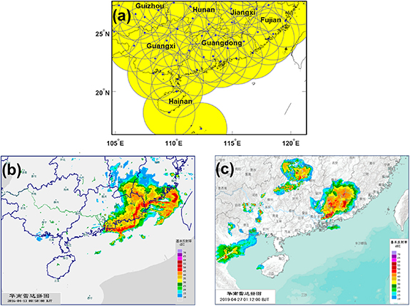
Figure 1. Radar reflectivity mosaic images over South China from CINRAD: (a) the South China region was observed by 49 weather radars (blue crosses, scanning areas shown in yellow) between the years 2009 and 2019; (b) the old image format used between 1st January 2009 and 14th June 2016; (c) the new format used since 15th June 2016.
Download figure:
Standard image High-resolution imageThe monthly precipitation dataset used in this study was from the Global Precipitation Climatology Project (GPCP v2.3, Adler et al 2018) at 2.5° × 2.5° resolution. Hourly surface concentration measurements of particulate matter (PM) with aerodynamic diameters ⩽2.5 μm (PM2.5) and ⩽10 μm (PM10) were from the China National Environmental Monitoring Centre (www.cnemc.cn), available from January 2013 to the present day. We used data from 276 surface sites over South China and applied a consistent quality control protocol to remove bad data and outliers (Jiang et al 2020).
2.2. Further quality control and extraction of radar reflectivity from mosaic images
Despite the CMA's preliminary data quality control, the historic radar mosaic reflectivity images were still occasionally defective or missing. We established a three-step data quality control protocol:
- (1)If the image at a default sampling time (00 min and 30 min of each hour) was missing, an image closest to and within 20 min of that sampling time, if available, was used. This protocol replaced 3.7%, 3.1%, and 1.1% of the default sampling time in March, April, and May, respectively.
- (2)Six types of defects were occasionally present in the sampled images: data loss, image output error, low-value reflectivity noise, radar scanning error, areas of abnormally high and discontinuous reflectivity, and non-precipitation echo at individual radars. Images with these defects were automatically detected and excluded. Each affected image was replaced by a non-defective image closest to and within 20 min of the default sampling time, if available. This protocol replaced 0.99%, 0.51%, and 0.46% of the mosaic images in March, April, and May, respectively.
- (3)If no replacement image was available, that sampling time was defined as invalid. Overall, 11%, 13%, and 10% of the sampling times were defined as invalid in March, April, and May during 2009–2019, respectively.
In the end, valid historic mosaic images were available for over 60% of each month's sampling time, except for April 2012 due to memory faults (13% valid rate, figure S1). We concluded that the valid images provided a sufficient temporal coverage and were representative of the climatology of springtime radar reflectivity over South China from 2009 to 2019. Finally, we extracted reflectivity data by removing the auxiliary geographical information, such as administrative boundaries and city names, from the mosaic images (figure S2). This procedure created false discontinuity by breaking the contiguous reflectivity signals into fragments; the discontinued pixels were filled by interpolating the eight surrounding grids. The corrected images retained the reflectivity features (figures S3(b) and (d)) and were used for further analyses.
2.3. Objective diagnostic algorithm for MCSs based on radar reflectivity
We defined the convective precipitation area associated with a mature MCS as a contiguous area in a radar mosaic image satisfying the following criteria (Parker and Johnson 2000): (1) all pixels within that contiguous area had a radar reflectivity of ⩾40 dBZ; (2) at least one pixel (approximately 4.4 km2 in size) within that contiguous area had a radar reflectivity of ⩾50 dBZ; (3) the contiguous area extended ⩾100 km in at least one horizontal direction. Additionally, we defined the area of stratified precipitation associated with that MCS as pixels with radar reflectivity ⩾25 dBZ but <40 dBZ and adjacent to the aforementioned contiguous area (figure S4(c)). We also calculated the convective precipitation area ratio (CPR, value ranging from 0 to 1) of an MCS, defined as the ratio of its convective precipitation area (⩾40 dBZ) relative to its total (convective plus stratified) precipitation area. An MCS with CPR ⩾0.5 indicated that its precipitating area was mostly convective.
Figure S4 illustrates the diagnostic process of mature MCS using a single radar reflectivity mosaic image at a specific time. Figure S5 shows examples of mature springtime MCSs over South China as identified by our algorithm. We labeled each contiguous area that met our MCS criteria as an individual mature MCS (figure S4(a)). The monthly half-hour counts of MCSs referred to the total number of MCSs detected at half-hour intervals during that month. We recorded the location and size of each MCS and determined its length-to-width ratio (LWR, the ratio of the major axis to the minor axis) by fitting it to an ellipse (figure S4(b)). An MCS with an LWR ⩾5 is typically identified as linear (i.e. a squall line), while an LWR between 2 and 5 indicates a quasi-linear MCS. An LWR <2 indicates a circular MCS (also known a mesoscale convective complex, MCC) (Geerts 1998, Parker and Johnson 2000, Haberlie and Ashley 2019). MCSs often include a stratiform precipitation area that trails (TS), leads (LS), or is parallel to (PS) the convective precipitation area, and each of these three MCS archetypes demonstrated distinct dynamic structures (Parker and Johnson 2000). We defined the PS MCS as those where the center of the stratiform precipitation area falls along the major axis of the MCS. We defined the TS and LS MCSs as those where the centers of the stratiform precipitation area fall behind and ahead of the convective precipitation area, respectively.
3. Climatological features of springtime MCSs over South China and the interannual variation of those features
Using the algorithm described in section 2.3, we identified a total of 7615 half-hour counts of springtime MCSs during 2009 and 2019. The spatial distributions of detected MCSs varied notably from March to May during 2009–2019 (figure 2). In March, MCSs were detected most frequently over central Guangdong and the southern parts of Jiangxi Province. In April, MCSs were mostly along the coast of eastern Guangdong Province. In May, MCSs were detected most frequently over the Pearl River Delta and the western part of Guizhou Province. Most MCSs moved eastward due to the prevailing westerly in the region. These characteristics constituted a climatology for seasonal heavy rainfall over South China (Luo et al 2020a).
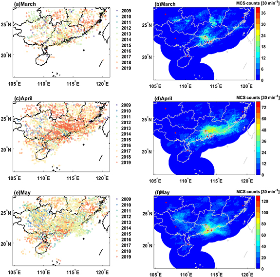
Figure 2. Spatial distributions of springtime MCSs over South China in (a) March, (c) April, and (e) May during 2009–2019. Circles indicate the center of each MCS detected at half-hour intervals, color-coded by the year. Also shown are the total half-hour counts of MCSs in each pixel (approximately 2.1 km resolution) in (b) March, (d) April, and (f) May during the study period. The red crosses indicate provincial capital cities, and the dark gray lines indicate administrative boundaries and the Pearl River.
Download figure:
Standard image High-resolution imageThe mean monthly half-hour counts of MCSs in March, April, and May were 103 ± 83, 274 ± 298 (excluding 2012), and 337 ± 225, respectively, with great intreannual variability (figures 3(a)–(c)). The occurrences of MCSs were most frequent in May. Excluding 2012, March and April MCSs occurred least frequently in 2010, 2011, 2015, and most frequently in 2016. In May, MCS counts were lowest in 2011 and highest in 2015. These differences were not caused by the variation of data availability (figure S1(a)) and more likely reflected the seasonal and interannual variation in the regional atmospheric thermodynamics. There were no statistically significant trends for the monthly mean MCS counts during 2009–2019. For each of the three months, the interannual variabilty of MCS counts were highly correlated with year-to-year variability of precipitation (r = 0.82, 0.73, and 0.71, respectively, excluding April 2012), indicating that MCSs were the main contributor to springtime precipitation over South China (Luo et al 2013).

Figure 3. Statistics of springtime MCS features over South China in March (left panel), April (center panel), and May (right panel) during 2009–2019. (a)–(c) Monthly half-hour counts of MCSs [unit: # 30 min−1]. The blue solid lines and the green dashed lines indicated the timeseries of monthly precipitation and their linear trends during 2009–2019, respectively. The temporal correlations (r) between monthly precipitation and MCS counts are shown inset. (d)–(f) Box plots of MCS sizes [km2]. (g)–(i) Box plots of MCS major axis lengths [km]. (j)–(l) Box plots of MCS length-width ratios (LWR). The dotted blue line indicates LWR = 5. (m)–(o) Box plots of MCS orientations, defined as the angle between the north and the MCS's major axis. The blue dotted lines indicate the mean values.
Download figure:
Standard image High-resolution imageFigures 3(d)–(f) show the morphology and structure of springtime MCSs over South China. The average areas of MCSs in March, April, and May were 3884 ± 3025 km2, 4210 ± 3551 km2, and 3487 ± 2564 km2, respectively, again with large interannual variability. The mean horizontal lengths of the MCSs along their major (longest) axis were 153 ± 65 km, 164 ± 69 km, and 152 ± 59 km in March, April, and May, respectively (figures 3(g)–(i)). Figures 3(m)–(o) show the orientation of the detected springtime MCSs, defined as the angle between the north and the MCS major axis. The mean orientation of MCSs was 41° ± 36°, 34° ± 42 °, 30° ± 52° in March, April, and May, respectively, indicating that most springtime MCSs over South China oriented in a northeast-southwest direction.
Figures 3(j)–(l) show the LWRs of springtime MCSs over South China. The mean LWR for all springtime MCSs over South China was 3.4 ± 1.5, and 72% of the springtime MCSs were quasi-linear with LWRs between 2 and 5. The percentage of MCSs taking the form of squall lines (i.e. linear with LWRs ⩾5) in March, April, and May were 20%, 16% and 17%, respectively. Only 11% of the analyzed MCSs in spring had LWRs <2. Moreover, circular MCSs in March and April tended to occur in the years when MCSs occurred less frequently (2011 and 2015). This finding suggested that the regional atmospheric dynamics in March and April of 2011 and 2015 may be different from those in the other years during our study period. We analyzed the correlations among the different features of MCSs (figure S6) and found that MCSs with longer major axis lengths were more likely to be linear/quasi-linear, of larger size, and in a northeast-southwest orientation.
Figures 4(a)–(c) show the CPRs of springtime MCSs over South China. The CPRs for springtime MCSs over South China averaged 0.34 ± 0.16. Sixty-one percent of the MCSs had CPRs between 0.2–0.5. The percentages of MCSs dominated by convective area (CPR ⩾ 0.5) were 12%, 23% and 15%, respectively, in March, April, and May. We found that the median CPRs of MCSs showed a small, but significant positive trend in May (0.01 yr−1, p-value = 0.02) between 2009 and 2019, potentially indicating an expansion of the MCSs' convective area in May during this period.
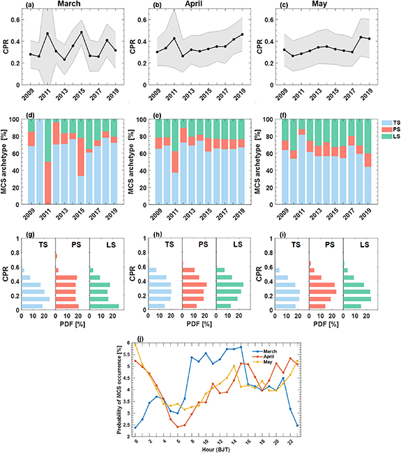
Figure 4. Statistics of springtime MCS features over South China in March (left panel), April (center panel), and May (right panel) during 2009–2019. (a)–(c) The convective precipitation area ratios (CPRs) of MCSs. The shaded areas indicate the standard deviations, and the black lines indicate the mean. (d)–(f) The percentages of the three MCS archetypes, in which the stratiform precipitation area is trailing (TS, blue), parallel (PS, orange) to, or leading (LS, green) the convective precipitation area. (g)–(i) The probability distribution functions (PDF) of CPR for the three MCS archetypes. (j) The diurnal probability distributions of MCS half-hour counts in March (blue), April (red), and May (yellow) during the years 2009–2019. The local time is shown as Beijing Standard Time.
Download figure:
Standard image High-resolution imageFigures 4(d)–(f) show that the TS archetype was dominant for springtime MCS over South China, consistent with the finding of Chen et al (2022). The mean percentages of the three MCS archetypes (TS, PS, LS) during our study period were 63%,17%, 20% in March, 65%, 13%, 22% in April, and 60%, 12%, 28% in May, respectively. Previous studies have shown that TS MCSs tend to be associated with stronger cold pool strengths, larger propagation speeds, and longer durations compared to PS and LS MCSs. This was because the mid-troposphere advection of hydrometers towards the MCSs from the rear was larger in TS MCSs (Parker and Johnson 2000). Additionally, we found that during the years when March and April MCSs were infrequent, the archetype of MCSs were also considerably different than the MCSs in other years. In March of 2011 and 2015 and in April 2011, PS MCSs occurred more frequently while TS MCSs less frequently. In March 2010, however, all detected MCSs were of a TS archetype. The probability distributions of CPR for the three MCS archetypes varied from month to month (figures 4(g)–(i)). The TS archetype in March tended to have lower CPR. In April, all three archetypes were likely to have higher CPRs compared to May.
Figure 4(j) shows the diurnal probability distributions of springtime MCS occurrences over South China. In March, MCSs were most frequent mid-day (8:00–15:00) and least frequent at night (22:00–1:00 the following day local time). In contrast, in April and May, MCSs were most frequent around midnight and least frequent in the early morning (4:00–8:00 local time). Combined with the observation that MCSs mostly occurred in the coastal area in April and May (figures 2(d) and (f)), the nighttime occurrences of MCSs in April and May likely reflected their trigger by the sea-land breeze and the nighttime double low-level jet along the coast (Du and Chen 2019, Luo et al 2020a).
4. Potential connection between MCS occurrences and surface aerosol abundances over South China in spring
Figure 5 and table 1 show the monthly means and interannual variations of observed surface PM2.5 and PM10 concentrations over South China in March, April, and May of 2013–2019. Surface PM concentrations had decreased in most parts of China between 2013 and 2019 as a result of China's aggressive pollutant emission control (Jiang et al 2020). This improvement of air quality over South China was apparent in figure 5. Monthly mean surface PM2.5 concentrations in March, April, and May decreased significantly at rates of −2.8 ± 0.0 μg m−3 yr−1, −2.9 ± 0.0 μg m−3 yr−1, and −0.76 ± 0.0 μg m−3 yr−1, respectively. Monthly mean surface PM10 concentrations in March and April decreased significantly at rates of −4.1 ± 0.0 μg m−3 yr−1 and −3.2 ± 0.0 μg m−3 yr−1 during the study period. The monthly mean surface PM10 concentrations in May were relatively low and showed no significant trend between 2013 and 2019 (figure 5).

Figure 5. Time series of MCS occurrences and air quality in spring over South China in March (top panel), April (middle panel), and May (bottom panel) during 2013–2019. (a)–(c) The monthly half-hour counts of MCSs (grey bars), the time series of monthly mean PM2.5 concentrations (blue), and the monthly numbers of clean (green) and polluted (orange) days. The correlation coefficient (r) between MCS counts and the different pollution level metrics are shown inset. (d)–(f) Similar to (a)–(c), but for PM10.
Download figure:
Standard image High-resolution imageTable 1. Correlation coefficients (r) between monthly MCS half-hour counts and monthly mean surface PM concentrations or monthly numbers of clean/polluted days over South China in March, April, and May of 2013–2019.
| March | April | May | |
|---|---|---|---|
| Monthly mean surface PM2.5 concentrations between 2013 and 2019 (μg m−3) | 40 ± 13 | 36 ± 11 | 29 ± 7 |
| r(MCS counts, monthly mean PM2.5 concentration) for 2013–2019 | 0.54 | −0.68 | 0.38 |
| Bottom/top terciles of daily PM2.5 concentrations between 2013 and 2019 (μg m−3) | 34/44 | 29/40 | 25/32 |
|
r(MCS counts, monthly numbers of clean days | −0.20 | 0.80 | −0.21 |
|
r(MCS counts, monthly numbers of polluted days | 0.79 | −0.75 ** | 0.14 |
| Monthly mean surface PM10 concentrations between 2013 and 2019 (μg m−3) | 63 ± 21 | 60 ± 18 | 51 ± 12 |
| r(MCS counts, monthly mean PM10 concentration) for 2013–2019 | 0.58 | −0.80 | −0.31 |
| Bottom/top terciles of daily PM10 concentrations between 2013 and 2019 (μg m−3) | 53/68 | 50/66 | 45/56 |
|
r(MCS counts, monthly numbers of clean days | −0.19 | 0.82 | 0.06 |
|
r(MCS counts, monthly numbers of polluted days | 0.77 | −0.82 | −0.47 |
* : two-tail p-value < 0.05; **: two-tail p-value < 0.1. a Clean days were defined as the days on which the daily mean PM2.5 or PM10 concentrations were below the bottom tercile concentration for a given month during 2013–2019. b Polluted days were defined as the days on which the daily mean PM2.5 or PM10 concentrations were above the top tercile concentration for a given month during 2013–2019.
We investigated how MCSs responded to the interannual variation of surface PM pollution. Figure 5 shows that, in April, the monthly half-hour counts of MCSs were negatively correlated with monthly mean concentrations of PM2.5 (r = − 0.68, p-value = 0.09) and PM10 (r = − 0.8, p-value = 0.03). However, these temporal correlations may not be robust, because surface PM concentrations in South China had dropped rapidly and the Pearson correlation coefficient is not resistant to extreme values.
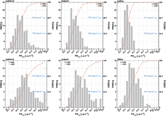
To address these robustness and resistance issues, we calculated the number of 'clean days' and 'polluted days' for a given month between 2013 and 2019. For each month, we defined the 'polluted' days as those on which the daily PM2.5 (or PM10) concentrations exceeded the top tercile (i.e. 67th percentile) of the pooled observations for that month; the 'clean' days were defined as those with daily PM2.5 (or PM10) concentrations lower than the bottom tercile (i.e. 33rd percentile) of the pooled observations (figure 6, table 1). During 2013–2019, the monthly numbers of polluted days declined significantly in March and April, while the monthly numbers of clean days increased significantly. There were no statistically significant trends for either the monthly number of polluted or clean days in May during the study period. These metrics of polluted and clean day numbers were resistant to extreme PM concentrations and reflected the interannual variation of air quality during the study period. In April during 2013–2019, the monthly half-hour counts of MCSs were positively correlated with the monthly numbers of clean days (r = 0.80 and 0.82 for PM2.5 and PM10, respectively; figure 5) and negatively correlated with the monthly numbers of polluted days (r = − 0.75 and −0.82 for PM2.5 and PM10, respectively) at 5% significance level. In contrast, in March, MCS counts were positively correlated with the numbers of polluted days (r = 0.79 and 0.77 for PM2.5 and PM10, respectively; figure 5). For the month of May, MCS occurrences were not correlated with the numbers of either clean or polluted days.
Figure 6. The probability distribution functions (PDF, grey bars) and cumulative probability distribution functions (CDF, red lines) of daily surface (a)–(c) PM2.5 and (d)–(f) PM10 concentrations at 276 sites over South China in March (left panel), April (middle panel), and May (right panel) for the years 2013–2019. For each given month, the bottom and top terciles for daily PM2.5 and PM10 concentrations during the study period are shown inset.
Download figure:
Standard image High-resolution image
The negative correlation between the numbers of polluted days and the counts of MCSs in April suggested that elevated levels of surface PM might have suppressed April MCS occurrences. This observed correlation tentatively aligned with the mechanism we proposed in a previous modeling study (Zhang et al 2020), wherein the direct and indirect radiative effects of anthropogenic aerosols both stabilized the lower atmosphere, which inhibited April MCS occurrence. Another possible explanation for the negative correlation between the number of polluted days and the MCS counts in April may be that infrequent MCSs weakened the scavenging of ambient PM. However, the significant positive correlation between the number of polluted days and MCS occurrences in March suggested that wet scavenging was not the sole interaction between surface PM abundance and MCSs.
Our previous modeling study (Zhang et al 2020) pointed out that aerosol may affect MCSs through aerosol's complex radiative and thermodynamic impacts on the regional atmosphere. We hypothesized that the varied correlations between surface PM abundance and MCS occurrences in different months reflected the seasonal differences in regional dynamic and thermodynamic conditions (Ding and Chan 2005, Luo et al 2020a). In March, South China is still strongly affected by the East Asian winter monsoon. By April, the strengths of cold continental air mass over East Asia and the warmer marine air mass over Northwestern Pacific are comparable, resulting in stationary fronts over South China, in which the MCSs are often embedded. These stationary fronts also produce extensive low cloud coverage, providing large leverage for the presence of aerosols to increase the liquid cloud optical depth and thus cool the surface (Zhang et al 2020). By May, the East Asian summer monsoon breaks out over South China, and the region experiences more convective precipitation and lower surface abundances of PM. These hypotheses highlighted the role of regional meteorological background in modulating the interactions between aerosols and MCSs and warrant further investigations.
5. Conclusions
This study analyzed historic radar reflectivity images to characterize springtime MCSs and their potential connections with surface aerosol abundance over South China. We found that the occurrences and morphology of springtime MCSs varied considerably seasonally and from year-to-year. Understanding the large-scale drivers of these variabilities may improve the accuracy of seasonal precipitation forecasts. We showed that the occurrences of MCSs over South China in April was negatively correlated regional PM pollution levels. This finding supports previous research indicating that high levels of anthropogenic aerosols suppress MCS occurrences in South China during April through aerosol-cloud-radiation interactions. Furthermore, although significant trend in April MCS occurrences was not observed during 2009–2019 due to its large interannual variability (figure 3(b)), the substantial and continued decline of surface PM since may potentially increase April MCS occurrences in the future. The potential connection between severe weather and air quality should be further investigated to enhance long-term disaster management and infrastructure planning. The objective diagnostic methodology of MCSs developed in this study can be applied to historical radar images from different parts of the world to improve our understanding of the trigger mechanisms, dynamics, and life cycles of MCSs.
Acknowledgments
This study was sponsored by the Natural Science Foundation of Shanghai (21ZR1462700), the National Natural Science Foundation of China (42325504), the Shenzhen Key Laboratory of Precision Measurement and Early Warning Technology for Urban Environmental Health Risks (ZDSYS20220606100604008), the Shenzhen Science and Technology Program (KQTD20210811090048025, JCYJ20220818100611024), the Guangdong University Research Project Science Team (2021KCXTD004), and the Guangdong Province Major Talent Program (2019CX01S188). Computational resources were provided by the Center for Computational Science and Engineering at the Southern University of Science and Technology.
Data availability statement
The GPCP monthly precipitation dataset is publicly available at www.esrl.noaa.gov/psd/data/gridded/data.gpcp.html. The mosaic images of radar reflectivity from CINRAD are available at www.nmc.cn/publish/radar/chinaall.html. Hourly surface concentration measumrents of PM are available at www.cnemc.cn.
Supplementary data (1.4 MB PDF)