

Abstract
Shipboard sampling of ocean biogeochemical properties is necessarily limited by logistical and practical constraints. As a result, the majority of observations are obtained for the spring/summer period and in regions relatively accessible from a major port. This limitation may bias the conceptual understanding we have of the spatial and seasonal variability in important components of the Earth system. Here we examine the influence of sampling bias on global estimates of carbon export flux by sub-sampling a biogeochemical model to simulate real, realistic and random sampling. We find that both the sparseness and the 'clumpy' character of shipboard flux observations generate errors in estimates of globally extrapolated export flux of up to ∼ ± 20%. The use of autonomous technologies, such as the Biogeochemical-Argo network, will reduce the uncertainty in global flux estimates to ∼ ± 3% by both increasing the sample size and reducing clumpiness in the spatial distribution of observations. Nevertheless, determining the climate change-driven trend in global export flux may be hampered due to the uncertainty introduced by interannual variability in sampling patterns.
Export citation and abstract BibTeX RIS

Original content from this work may be used under the terms of the Creative Commons Attribution 4.0 license. Any further distribution of this work must maintain attribution to the author(s) and the title of the work, journal citation and DOI.
1. Introduction
Organic matter generated via primary production (PP) in the surface ocean may sink into the mesopelagic zone and contribute to the oceanic sink of CO2. PP fixes ∼50–60 PgC yr−1 (1 Pg = 1 × 10¹⁵ g; Canadell et al 2021), however only a fraction of the particulate organic carbon (POC) created by primary producers sinks out of the upper ocean. This 'export flux' is then the starting point for a myriad of processes occurring in the mesopelagic, such as particle fragmentation (e.g. Briggs et al 2020), microbial respiration (e.g. Amano et al 2022) and zooplankton activity (e.g. Mayor et al 2020), that act to remineralise the POC. The remaining carbon reaching the deep ocean can be stored on climatically relevant timescales (e.g. Siegel et al 2021). Ocean–atmosphere model experiments have demonstrated that the biological carbon pump reduces atmospheric CO2 by ∼200 ppm at quasi-equilibrium (e.g. Parekh et al 2006), although more recent work has suggested this may be an overestimate of 30%–50% as feedbacks to the land biosphere are neglected (Oschlies 2009). The export flux can thus be viewed as ultimately setting the magnitude of carbon stored in the ocean via biotic activity.
Despite being a significant factor in the Earth's carbon cycle, the global magnitude of export flux is still poorly constrained, with estimates ranging from ∼5–12 PgC yr−1 (Henson et al 2011, Siegel et al 2014, DeVries and Weber 2017, Nowicki et al 2022, Clements et al 2023). In many cases, export flux estimates are derived by extrapolating from shipboard observations to the global scale via empirical relationships between flux and temperature, PP or other factors for which global data are readily available (Laws et al 2000, Dunne et al 2005, Henson et al 2012). Recently, machine learning approaches have also been used to extrapolate from scattered shipboard data to global scales (Clements et al 2023). Compilations of shipboard observations can contain hundreds of data points (Le Moigne et al 2013, Mouw et al 2016a, 2016b, Ceballos-Romero et al 2022). Commonly used methods are drifting sediment traps that capture the sinking particulate material, or assessment of the tracer thorium-234 (Th234) which is a proxy for the flux of POC (e.g. Baker et al 2020, Buesseler et al 2020, Estapa et al 2021, Roca-Martí et al 2021). However, due to logistical constraints, these shipboard observations are limited in their spatial and temporal coverage, and are also biased towards spring/summer and more readily accessible regions. In addition, shipboard observations tend to be very 'clumped' in space and time, with a high density of observations at the times and locations of process cruises. The patchiness of these data may underlie some of the large uncertainty in global export flux. For example, the estimates extrapolated from syntheses of Th234 observations (e.g. Henson et al 2011) tend to be at the low end of the range reported in the literature (∼5 PgC yr−1, with the literature range being ∼5–12 PgC yr−1). Bisson et al (2018) hypothesise that the characteristics of the Th234 dataset itself may be a driving factor as the data were collected primarily in low latitude regions.
The challenges of using sparse shipboard observations to derive global-scale fields of biogeochemical variables have previously been recognised. For example, sub-sampling a global ocean biogeochemistry model at the times and locations of shipboard pCO2 observations demonstrated that insufficient sampling both generates substantial biases in determining the trend of the ocean carbon sink (Hauck et al 2023) and imposes a fundamental limitation on robustly quantifying its decadal variability (Gloege et al 2021). Similarly, Bushinsky et al (2019) subsampled a high resolution biogeochemical model and found that differences in sampling density between ships and floats drove differences in the estimated Southern Ocean CO2 uptake. Here we address how data sparsity and spatial clumpiness may impact estimates of global carbon export flux. We do this by sub-sampling a global ocean biogeochemical model to simulate real, realistic and random sampling for export flux. Real sampling uses the dates and locations of shipboard data syntheses; realistic sampling uses the statistical characteristics of the real datasets to generate simulated sampling patterns; random sampling uses datapoints selected randomly in space and time. We compare the results of globally extrapolating the sub-sampled flux to the 'true' model flux to generate estimates of the uncertainty introduced by sparse spatial and temporal sampling of the ocean.
2. Methods
We sub-sample the MEDUSA model, which is an intermediate complexity biogeochemistry model (Yool et al 2013), coupled to the NEMO physical ocean model (Madec 2008). MEDUSA simulates the cycles of nitrogen, silicon, and iron. The plankton community consists of 'small' and 'large' fractions, where 'small' represents picophytoplankton and microzooplankton and 'large' represents diatoms and mesozooplankton. The particulate detritus is also divided into small, slow-sinking particles and large, fast-sinking particles, with small (large) particles being predominantly generated by the small (large) plankton. Full details of the model can be found in Yool et al (2013). In the configuration used here, the model is forced at the ocean surface with atmospheric output from the HadGEM2-ES Earth system model (Yool et al 2015). Although this simulation is driven by model-derived surface atmospheric forcing, rather than a reanalysis product derived from observations, it has previously been validated against observed biogeochemistry (e.g. Yool et al 2015) and we include plots comparing key biogeochemical parameters in the model and observations in figure S1. The model's use has already been established across a range of other studies (e.g. Asdar et al 2022, Jacobs et al 2021), including to examine spatial and temporal variability in export flux (Henson et al 2015, Giering et al 2017). Here we use the climatology of years 1982–2012 at 0.25° horizontal spatial resolution and 5 d temporal resolution.
Figure 1(a) shows the modelled POC export flux at 100 m depth (global total = 9.56 PgC yr−1, i.e. the summed export flux for the entire ocean for the whole climatological year). To extrapolate from sub-sampled points to the global scale, we follow the approach of numerous observation-based studies (e.g. Laws et al 2000, Dunne et al 2005, Henson et al 2011) and use the correlation between export and a different globally-resolved parameter, in this case net PP. Figure 1(b) shows that a strong linear relationship exists between export and PP in the model. We exploit this to reconstruct a global export flux field from the model PP (figure 1(c)); this flux has a very similar spatial pattern to the export flux simulated by MEDUSA, although a slightly higher global total export flux of 10.05 PgC yr−1. We refer to this reconstructed field in the rest of the manuscript as the 'true' model export flux. We use this value as the 'true' flux, rather than the model outputted export field, to accommodate the uncertainty introduced by applying the PP versus export regression, i.e. differences between the 'true' and extrapolated flux values are solely due to the effects of sub-sampling.
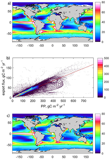
Figure 1. (a) Climatological annual export flux (gC m−2 yr−1) simulated by the MEDUSA model. Panel (b) plots the annual PP versus export flux for all ocean pixels (n = 649 979). Colour indicates number of datapoints (PP in bins of 2 gC m−2 yr−1 and export in bins of 0.5 gC m−2 yr−1). Linear regression (red line): export = 2.11(±0.025) + 0.21(±0.0002)*PP, r2 = 0.89, p < 1e−100. (c) Reconstructed annual export flux (gC m−2 yr−1) using the regression between PP and export. The reconstructed export shown in panel (c) is used as the baseline against which the fidelity of export derived by sub-sampling the model is assessed. We refer to the reconstructed export in panel (c) as the 'true' model export flux.
Download figure:
Standard image High-resolution imageFor each of the analyses described below, we use the PP and export data sub-sampled from the full model to establish a linear regression. The regression is then applied to the full model field of PP at each 5 d timestep (i.e. predicted export = intercept + gradient*5 d PP). The 5 d resolution predicted export fields are then summed over the year, and integrated globally accounting for the varying size of the model's grid cells to give the integrated total export flux.
We initially sub-sample the model at the dates (ignoring year) and locations of observations of Th234-derived flux at 100 ± 20 m depth (a typical depth for estimating export flux) contained in the dataset of (Mouw et al 2016a, 2016b), for which n = 375. The equivalent model depth level chosen spans ∼87–108 m. Then, to investigate the influence of the spatial bias in the dataset (i.e. shipboard data tend to be either in transects or multiple observations clustered in a small region), we simulate alternate sampling patterns that have similar statistical properties, i.e. whose angle, distance and time between samples are drawn from the same distribution, as the Mouw dataset. To do this, we first calculate the distances and angles (on a sphere) between subsequent points in the Mouw dataset and then use a kernel density function to estimate their respective probability distributions using the standard estimator formula:
where  are random samples drawn from the distances (and separately angles) of the Mouw dataset, which have an unknown distribution, n is the sample size,
  is the bandwidth of the Kernel smoothing window, and
  is the Kernel smoothing function, in this case a Gaussian function. A kernel density function approach was used to estimate the probability distributions of the distances and angles within the Mouw dataset as it allows a non-parametric estimation of probability distributions, important as no a priori assumptions about the form of the distributions needs to be made. A separate kernel density function was used to estimate the probability distribution of the time point sampled. We then randomly sampled a new set of distances and angles (and time points) from the distribution, and applied those to a randomly chosen initial location in the ocean. We repeated this sub-sampling 500 times to generate 500 simulated sampling patterns with similar statistical properties as the Mouw dataset. We generated these realistic sampling patterns for both global sampling, and sampling restricted to either subtropical or subpolar regions.
To test how sampling biases towards particular seasons might affect reconstructions of export flux, we used the 500 simulated sampling patterns to sample an increasing number of seasons. Each season was sampled with the same 500 patterns, so that the total number of datapoints increased from 500–2000 with the number of seasons sampled (i.e. from 1 to 4) and the sampling simulated repeated sampling of a single location, similar to observations at sustained observatories such as BATS (Bermuda Atlantic Time Series) or HOTS (Hawaii Ocean Time Series). We sampled just spring (March–May in Northern Hemisphere, September–November in Southern Hemisphere), then spring and summer (March–August/September–February), then spring and summer and autumn (March–November/September–May), and finally all seasons.
We also investigate the number of datapoints needed to reconstruct the 'true' model flux to a reasonable degree by randomly sub-sampling the model in both space and time for dataset sizes from 500–550 000 points. Finally, we examine how an alternate (non-ship based) approach to estimating carbon flux, the Biogeochemical-Argo (BGC-Argo) array, might affect estimates of global carbon flux. The BGC-Argo array consists of free-drifting floats that collect vertical profiles of water column properties every ∼10 d from ∼2000 m depth to the surface (www.biogeochemical-argo.org). Here, we sub-sample the model at the times and locations of BGC-Argo optical backscatter profiles, as backscatter can be used as a proxy for estimating POC fluxes (e.g. Briggs et al 2020, Henson et al 2023a, Terrats et al 2023).
3. Results and discussion
The applicability of the results presented here to real-world sampling of the global ocean depends on the model's ability to reproduce, to a reasonable degree, the real seasonality and spatial variability in export flux. Although there are insufficient observations of export flux to make a direct comparison, the model used here does simulate surface nutrients, chlorophyll and PP reasonably well (figure S1; Yool et al 2015). The choice of model is constrained to a simulation which has reasonably high spatial and temporal resolution (in this case, 0.25° and 5 d) to minimise uncertainties introduced by insufficient representation of the variability. As we expect real-world variability to be greater than in the model, the discrepancies between 'true' and extrapolated values shown here should be considered as a lower bound. If several different ocean biogeochemical models with similar resolution were available, the uncertainty in our analysis due to model structure (and not just the extrapolation effects) could also be assessed. The exact values of export, both 'true' and extrapolated, will depend on the model used, but nevertheless the comparison between the full and sub-sampled model presented here provides a useful insight into the influence of sampling bias.
Extrapolating the export flux generated by sub-sampling the model on the day of year and location of Th234 observations in the dataset of (Mouw et al 2016a) results in a total flux of 11.88 PgC yr−1, substantially higher (by 18%) than the 'true' model export of 10.05 PgC yr−1 (figure 2). (The PP vs export relationship for the sub-sampled points has r2 = 0.61, p ∼ 1 × 10−78.) This positive bias is not spatially uniform, with generally greater biases in the subtropical gyres, lower biases at temperate latitudes, and negative biases in several regions, including the equatorial Pacific and productive regions of the Southern Ocean.
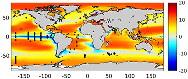
Figure 2. Difference in gC m−2 yr−1 between 'true' model export derived from the linear regression shown in Figure 1(b) and that derived using a PP versus export relationship obtained by sub-sampling the model at the day of year and locations of the Th234-based estimates of export flux at 100 ± 20 m depth (n = 375) reported in (Mouw et al 2016a), indicated by the black dots.
Download figure:
Standard image High-resolution imageThe observations in the Mouw dataset, as is common with all shipboard data, have a distinctive pattern, with both clumps of data points where field programmes have targeted a particular location, and lines of data points where transect cruises have been conducted. To examine whether the clumpiness inherent in typical syntheses of shipboard data results in a significant bias in export estimates, we generated 500 simulated sampling patterns. The statistical properties are similar to the Mouw dataset, but our simulated sampling does not include the biases associated with real shipboard data syntheses, in that our sampling patterns do not include biases stemming from the logistical constraints of shipboard operations (i.e. places within easy reach of a port or part of a repeat sampling programme, e.g. BATS, HOTS). The distribution of global total export flux reconstructed from the 500 simulated datasets is shown in figure 3(a). (The correlation coefficients of the PP vs export regressions range from 0.44 to 0.95 and all have a p-value < 1 × 10−39.) The median of the distribution (10.13 PgC yr−1) is quite similar to the 'true' model export (+0.8%), but the estimates have a large range, from 7.8 to 12.2 PgC yr−1 (−22.3–21.4%). The reconstructed export flux is thus sensitive to the spatial distribution of sampling which produces variations in the regression coefficients which, when globally extrapolated, can generate substantial differences in total estimated export flux. Some regions have consistent biases in reconstructed flux, even when they are sampled in the original dataset (figures 2 and 3(d)), such as the equatorial Pacific, eastern boundary upwelling zones and subpolar-subtropical gyre boundaries. Other regions display the opposite behaviour, where they consistently have low biases in reconstructed flux, even if they are not well-sampled (or sampled at all) in the original dataset, such as the oligotrophic gyres. Furthermore, if sampling is confined to low latitudes the median global flux is substantially lower (by 11.4%) than the 'true' value (8.9 PgC yr−1, range of 6.98–11.14 PgC yr−1 (−30.5 to +10.8%)) and vice versa for sampling confined to high latitudes (10.94 PgC yr−1 (8.9% greater than 'true' value), range of 7.1–12.92 PgC yr−1 (−29.4–28.6%); figure S2). The range of possible values is also lower when sampling only in the low latitudes. One-off sampling of regions with dynamic export regimes thus results in greater biases, and higher extrapolated flux estimates, than one-off sampling of more seasonally invariant regions.
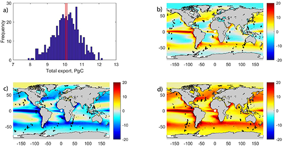
Figure 3. Five hundred simulated shipboard sampling patterns were created (see methods section). Panel (a) shows the distribution of the reconstructed global export flux for all 500 simulated sampling patterns. Red lines mark the 'true' model export (10.05 PgC yr−1) and median reconstructed export (10.13 PgC yr−1). Panels (b)–(d) show the difference (in gC m−2 yr−1) between 'true' model export from the linear regression shown in Figure 1(b) and that derived using a PP versus export relationship obtained by sub-sampling the model at the points shown by the black dots. The reconstructed global patterns shown are for the sub-sampled pattern: (b) for which the global total export is closest to the median export of the 500 sampling patterns (10.12 PgC yr−1); (c) the smallest simulated global export flux (7.86 PgC yr−1); (d) the largest simulated global export flux (12.20 PgC yr−1).
Download figure:
Standard image High-resolution imageExamination of the simulated sampling patterns from across the distribution in figure 3(a) does not suggest that any particular pattern is more likely to result in a truer estimate of total global flux. For example, there is no relation between the number of biomes sampled and the discrepancy between reconstructed and 'true' export flux (figure S3). Is the sensitivity of global flux estimates extrapolated from shipboard datasets due only to their relatively small size, or does the clumpiness also play a role? We explore this question by sub-sampling the model at random locations with increasing dataset size from 500–550 000 points. The global total export flux reconstructed by random sampling is not strongly dependent on the number of samples, with median values of total global export varying only between 9.98–10 PgC yr−1 when increasing the sample size from 500 to 500 000 points (figure 4(a)). (The correlation coefficients of the PP vs export regressions range from 0.65 to 0.88 and all have a p-value < 1 × 10−38.) However, the range in possible values (as determined by repeating the random sub-sampling 500 times for each sample size, shown as whiskers in figure 4(a)) decreases substantially as the sample size increases. Nevertheless, the range in total global export reconstructed from just 500 random points is 9.47–10.53 PgC yr−1 (−5.8 to 4.8%%), i.e. still considerably narrower than the range generated by simulating the clumpiness of shipboard sampling based on the Mouw dataset.
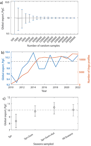
Figure 4. (a) Global total export reconstructed from an increasing number of randomly sampled data points, with the whiskers representing the range in export generated by repeating the sampling procedure 500 times (i.e. generating a different, randomly distributed, dataset on each iteration). (b) Number of BGC-Argo particle backscattering profiles in each year (orange) and total export reconstructed from sub-sampling the full model at the times and locations of those profiles (blue). (c) Global export reconstructed from clumpy sampling of an increasing number of seasons (see methods); spring (Spr), summer (Sum), autumn (Aut). Circles are the median value and whiskers represent the range in export generated by repeating the sampling procedure 500 times. Dashed line indicates the 'true' global export flux.
Download figure:
Standard image High-resolution image
Our analysis suggests that generating a well-constrained estimate of global export requires thousands of data points, ideally randomly distributed over the global ocean. The logistical constraints on shipboard sampling mean that this ideal is unlikely to be achieved. However, the advent of autonomous technologies, including BGC-Argo floats and gliders, offer the opportunity to overcome this barrier and significantly increase the dataset size and spatial coverage. Converting optical backscatter data into estimates of particle flux necessarily carries an additional uncertainty (e.g. Briggs et al 2011, Giering et al 2020), but provided the dataset is internally consistent this should be outweighed by the benefits of a vastly larger dataset. To evaluate this, we sub-sample the modelled export flux and PP at the dates and locations of BGC-Argo backscatter profiles between 2010 and 2022 (note that we sub-sample the repeating, climatological model year so that differences in extrapolated flux values are solely due to changing sampling patterns). The BGC-Argo sampling density is initially relatively low and the globally extrapolated export flux value is lower than the 'true' value (figure 4(b)). As the BGC-Argo network becomes denser in later years (figure S4) and the number of profiles increases concomitantly, the extrapolated export flux becomes closer to the 'true' value. Once the number of profiles exceeds ∼5000 in 2013, the extrapolated flux oscillates around the 'true' value. From 2015–2022, the number of profiles per year was between 10 000 and 12 000, and the total extrapolated export flux ranged between 9.78 and 10.28 PgC yr−1 (−2.7–2.3%). (The correlation coefficients of the PP vs export regressions range from 0.64 to 0.84 and all have a p-value < 1 × 10−65.) However, there is no direct correspondence between the number of profiles and the veracity of the total global export.
As an important and interesting aside, if the PP versus export equation derived from sub-sampling the model is applied to the annual total PP (rather than the 5 d PP), estimated global total fluxes are significantly larger than the 'true' values. In the case of the (Mouw et al 2016a) sub-sampling, the estimated flux becomes 20.83 PgC yr−1, over double the 'true' model export. This raises an important methodological point: when calculating extrapolated fluxes, the derived empirical relationships should be applied to time-varying predictor variables (not annual mean), followed by integrating through the year to generate the annual total. This result also points to the importance of capturing the seasonality of fluxes in order to robustly generate global scale estimates.
Although many ship-based data syntheses have a bias towards spring and summer sampling, autonomous platforms, such as the BGC-Argo floats, do not suffer from the same logistical restrictions and so provide a more complete picture of the seasonality of fluxes. Figure 4(c) shows the influence of sampling an increasing number of seasons, from spring only through to all seasons, where each season is sampled 500 times using the realistic, i.e. clumpy, sampling patterns (sampling 2 seasons = 1000 locations, 3 seasons = 1500 locations). Sampling throughout the year at 2000 locations generates a reconstructed median global flux of 10.07 PgC yr−1, i.e. almost identical to the 'true' flux, although the range in possible values is large (9.12–10.88 PgC yr−1 ≡ −9.4 to 8.0%). Intriguingly, sampling only in spring and summer at 1000 locations achieves a median global flux of 9.85 PgC yr−1, only 2% smaller than the 'true' flux, presumably because the majority of flux occurs during the productive spring and summer months. However, the range of possible values is still fairly large (9.09–10.69 PgC yr−1 ≡ −7.7 to 8.5%). The sampling patterns for which the global flux is closest to the 'true' value for the two cases have little similarity (figure S5), again emphasising that the extrapolated flux is strongly dependent on the exact locations sampled. However, sampling in the spring only results in a noticeably lower median value and, importantly, the range in possible values does not include the 'true' export flux (8.36 PgC yr−1, range 7.34–9.41 PgC yr−1).
4. Conclusions
Here we examine how seasonal and spatial biases in in situ observations of export flux may affect the derivation of global-scale flux estimates. In previous studies, global extrapolation of scattered observations has been achieved by establishing an empirical relationship between flux and variables that are readily obtained on a global scale (usually satellite-derived data), such as temperature or PP. We follow a similar approach here by sub-sampling a global biogeochemical model to replicate patterns of observational data syntheses, using a linear regression between export and PP to extrapolate to a global scale, and then comparing this derived estimate of total export flux to the 'true' model export.
In our analysis, the total global export extrapolated by sub-sampling the model in a way that replicates shipboard observations is sensitive to the specific locations sampled (figure 3), varying from −22.3 to +21.4% from the 'true' value. Randomly sampling the ocean generates a much lower sensitivity to the exact locations sampled, particularly if total sample size is in the thousands rather than the hundreds, e.g. total export varies from −2.2 to +0.9% from the 'true' value for 5000 datapoints (figure 4(a)). This implies that the global total extrapolated flux varies significantly as a consequence of both the relatively small sample size of shipboard data syntheses and their inherent clumpiness.
Our results imply that thousands of carbon flux measurements are needed to robustly estimate global export flux, compared to the hundreds currently available. It is thus unlikely that shipboard observations alone will achieve the required data density, at least in the near future. The vastly increased data volumes generated by autonomous vehicles will be necessary, although this comes with its own challenges associated with deriving robust flux estimates from proxies such as optical backscatter (e.g. Briggs et al 2011). Nevertheless, it is likely that exploiting the BGC-Argo network (for spatial coverage), perhaps combined with intensive localised sampling (for high temporal resolution) by gliders will permit sufficient observations to derive more robust export fluxes. Shipboard observations will still be necessary to provide data for calibration and validation of autonomous-derived estimates, and satellite data will still be needed for global scaling-up, perhaps incorporating machine learning (Clements et al 2022) or spatio-temporal modelling techniques (Yarger et al 2022) to maximise predictive power.
For clumpy and sparse sampling, i.e. simulating shipboard data syntheses, the range in global extrapolated export flux is 7.8–12.2 PgC yr−1. The range in previously published global export flux based on observations-based extrapolations and other approaches such as data-constrained food web models or biogeochemical tracer inversions is ∼5–12 PgC yr−1 (Laws et al 2000, Henson et al 2011, Siegel et al 2014, DeVries and Weber 2017). Despite >20 years of effort with multiple different approaches based on shipboard data, the range in global export flux is still poorly constrained. In comparison, the range in global export flux based on extrapolation of BGC-Argo profiles—which are both significantly more numerous and more evenly spread spatially—is highly constrained when the annual number of profiles exceeds ∼10 000 (9.8–10.3 PgC yr−1). However, in terms of our ability to detect long-term change with contemporary flux datasets, it is worth noting that the range of 0.5 PgC yr−1 in export flux driven by interannually variable sampling patterns in the BGC-Argo network is greater than the majority of CMIP6 models predict to be the future climate trend in export; 13 of 19 CMIP6 models reporting export flux predict globally-integrated export flux to change by less than 0.5 PgC yr−1 by the end of the century (average of 2091–2100 minus average of 1850–1900; Henson et al 2022). Detecting a climate change-driven trend in export flux on global scales may thus be challenging given the fluctuations in flux extrapolated from current observing systems, driven by interannual variability in sampling patterns.
Our results suggest that current shipboard data syntheses are insufficient to generate global scale export flux extrapolations. However, our results also emphasise the potential of autonomous vehicle-based datasets to overcome these limitations and generate significantly more robust estimates of global-scale POC fluxes.
Acknowledgments
S H was supported by a European Research Council Consolidator Grant (GOCART, Agreement Number 724416), co-funding from the European Union, Horizon Europe Funding programme and UK Research and Innovation (OceanICU, Agreement Number 101083922) and by Natural Environment Research Council Grants (BRICS, NE/X00855X/1 and GLOBESINK, NE/X008657/1). M L H received support from Anillo BiodUCCT (ATE220044). A M was supported by Natural Environment Research Council grant CUSTARD (NE/P021247/2). A Y received support from Natural Environment Research Council grants TerraFIRMA LTSM (NE/W004895/1), CLASS LTSS (NE/R015953/1) and ESM LTSM (NE/N018036/1).
Data availability statements
The data that support the findings of this study are openly available at the following URL/DOI: https://zenodo.org/record/8279110 (Henson et al 2023b).
Supplementary data (0.8 MB PDF)