

Abstract
Climate change poses a serious threat to permafrost integrity, with expected warmer winters and increased precipitation, both raising permafrost temperatures and active layer thickness. Under ice-rich conditions, this can lead to increased thermokarst activity and a consequential transfer of soil organic matter to tundra ponds. Although these ponds are known as hotspots for CO2 and CH4 emissions, the dominant carbon sources for the production of greenhouse gases (GHGs) are still poorly studied, leading to uncertainty about their positive feedback to climate warming. This study investigates the potential for lateral thermo-erosion to cause increased GHG emissions from small and shallow tundra ponds found in Arctic ice-wedge polygonal landscapes. Detailed mapping of fine-scale erosive features revealed their strong impact on pond limnological characteristics. In addition to increasing organic matter inputs, providing carbon to heterotrophic microorganisms responsible for GHG production, thermokarst soil erosion also increases shore instability and water turbidity, limiting the establishment of aquatic vegetation—conditions that greatly increase GHG emissions from these aquatic systems. Ponds with more than 40% of the shoreline affected by lateral erosion experienced significantly higher rates of GHG emissions (∼1200 mmol CO2 m−2 yr−1 and ∼250 mmol CH4 m−2 yr−1) compared to ponds with no active shore erosion (∼30 mmol m−2 yr−1 for both GHG). Although most GHGs emitted as CO2 and CH4 had a modern radiocarbon signature, source apportionment models implied an increased importance of terrestrial carbon being emitted from ponds with erosive shorelines. If primary producers are unable to overcome the limitations associated with permafrost disturbances, this contribution of older carbon stocks may become more significant with rising permafrost temperatures.
Export citation and abstract BibTeX RIS

Original content from this work may be used under the terms of the Creative Commons Attribution 4.0 license. Any further distribution of this work must maintain attribution to the author(s) and the title of the work, journal citation and DOI.
1. Introduction
In recent decades, air and permafrost temperatures have steadily increased throughout the Arctic (Overland et al 2018, Biskaborn et al 2019). As vast areas of permafrost are composed of sediments consolidated by ice, thawing permafrost induces major geomorphological changes across these regions (Romanovsky et al 2017). Both gradual and sudden disturbances mobilise organic matter stored in permafrost for centuries to millennia (Schuur et al 2015, Turetsky et al 2020). These stocks become exposed to microbial and photochemical transformation, especially after being transported to aquatic systems (Cory et al 2013, Vonk et al 2015). Effects of permafrost thaw on soil organic matter (SOM) mobilisation and mineralisation have not been studied extensively in Arctic lowlands, where numerous shallow ponds form on organic-rich ice-wedge polygonal landscapes (Muster et al 2017). Nevertheless, several studies have shown that these small water bodies are hotspots for greenhouse gas (GHG) emissions (e.g. Laurion et al 2010, Sepulveda-Jauregui et al 2015, Prėskienis et al 2021, Beckebanze et al 2022). Conditions are favourable for carbon degraders in these ecosystems due to sufficient heat accumulation during summer days, large soil-water contact promoting direct leaching of nutrients and SOM, and unstable shorelines bringing freshly thawed SOM into the water column (Jeppesen et al 2021).
Although ponds and lakes located in permafrost regions are recognised as large carbon emitters to the atmosphere (e.g. Abnizova et al 2012, Pokrovsky et al 2013, Serikova et al 2019), their feedback effect on climate has been considered negligible due to their small surface area globally (Wik et al 2016, Polishchuk et al 2018), or due to the emitted carbon being predominantly modern (Elder et al 2018, Dean et al 2020). Nevertheless, the increasing rate of permafrost thaw has been shown to transform these organic-rich landscapes from carbon sinks to carbon sources (Kuhn et al 2018), and to promote carbon emissions in the form of CH4 (Anisimov 2007, Knoblauch et al 2018). As CH4 is a more potent GHG than CO2 (Nisbet et al 2019), any conditions favouring an increasing ratio of CH4 to CO2 emissions may be considered as positive feedback to climate warming. GHG fluxes from Arctic freshwater bodies are relatively underreported and highly variable, both temporally and spatially (Emmerton et al 2016, Jansen et al 2019, Prėskienis et al 2021), further complicating the assessment of their impact on the global carbon cycle.
The effects of shore erosion or general thermokarstic activity on the limnology of tundra ponds have already been explored by previous studies. In the Lena delta, for example, tundra ponds with permafrost disturbances in surrounding polygons have exhibited two to three orders of magnitude higher emissions of CH4 (Langer et al 2015). On Melville Island (western Nunavut), permafrost disturbances have been reported to impact tundra pond geochemistry and increase dissolved CO2 (Heslop et al 2021). Nevertheless, quantitative assessments linking landscape disturbance due to permafrost thaw with GHG emissions from Arctic ponds have never been done before. The aim of this study, therefore, was to investigate the carbon sources driving GHG production in tundra ponds formed on organic- and ice-rich Holocene sediments on Bylot Island, with a focus on the effects of thermokarstic shore erosion. We hypothesised that it would have a significant impact on the limnological functioning of small aquatic systems (including temperature, oxygen, light, organic matter, and nutrients), creating favourable conditions for higher CO2 and CH4 emissions through effects on the balance between heterotrophic and phototrophic production. In addition to studying the links between erosion intensity, pond limnology and GHG emission rates, carbon sources were traced using 13C and 14C isotopes to further explore the modern and ancient carbon pools that drive GHG production in these shallow aquatic ecosystems.
2. Methods
2.1. Study site and study design
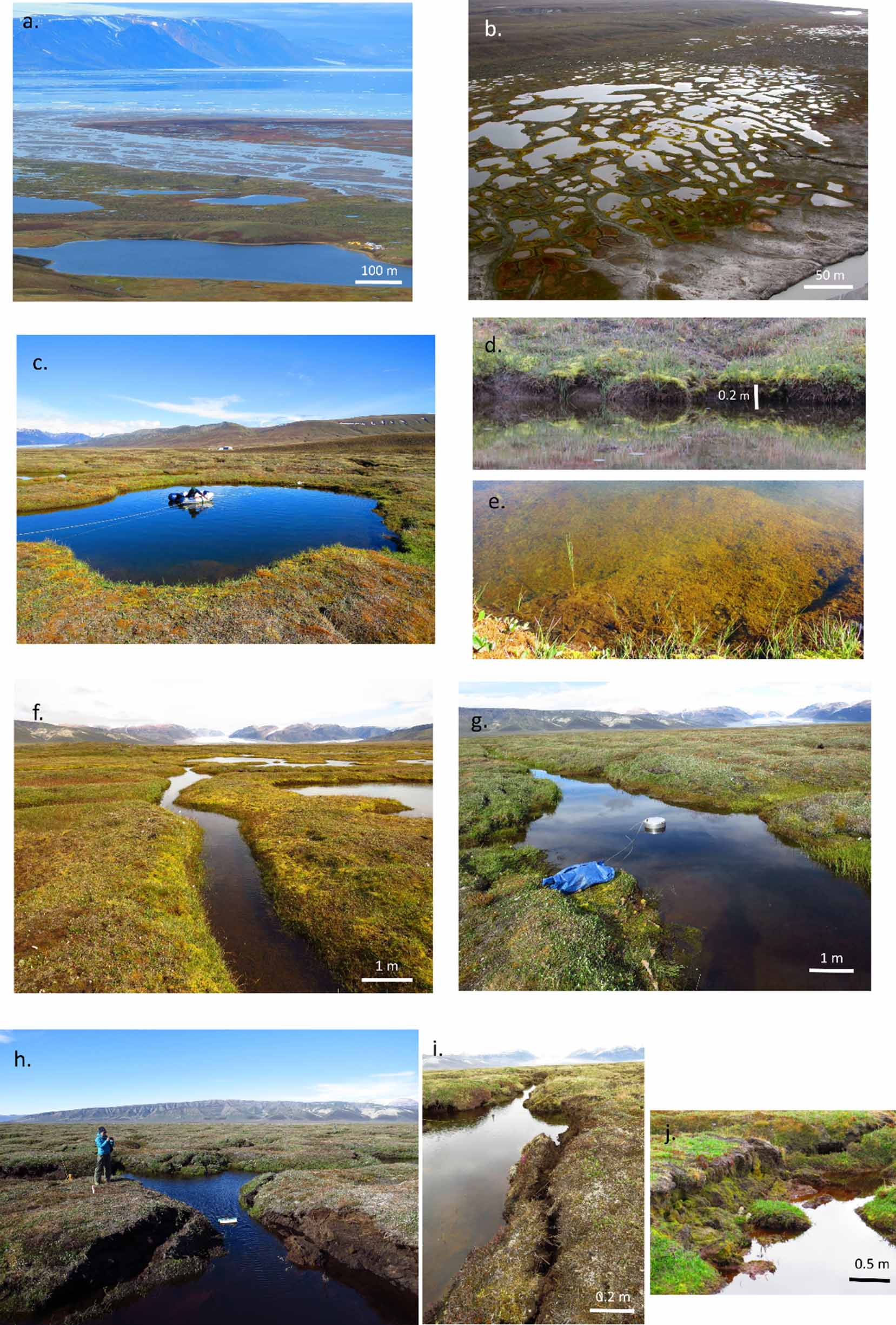
The studied ponds are located in the periglacial valley of Qarlikturvik (glacier C-79; 73°09ʹ N, 79°58ʹ W) on the western side of Bylot Island, in the Canadian Arctic Archipelago. The region experiences a polar climate, with long and cold winters, and low annual precipitation. The valley is dominated by a proglacial river (figure 1(a)); its outwash plain is bordered by a 3–5 m thick aggradation terrace composed of a mixture of late Holocene peat and aeolian deposits (silt and fine sand; Fortier et al 2006). The terrace is underlain by cold deep continuous syngenetic permafrost with a complex network of ice-wedge polygons (Fortier and Allard 2004). The irregular surface of the polygonal landscape accommodates accumulation of snow and water, leading to formation of thousands of small, shallow water bodies (0.1–1.3 m deep; figure 1(b)), here referred to as tundra ponds.

Figure 1. Photographs illustrating the landscape of the study site (a), (b) and the variability of studied ponds and their shore erosion levels (c)–(j). The coalescent polygon ponds (c) are characterised by low but steep shores with some outcrops (d), and flat bottoms covered with benthic mats (e). The ice-wedge trough ponds feature a wide range of shore stability, from no erosion (f), and stabilised re-vegetated shores (g), to high erosion with falling and slumping peat blocks (h), (i) and recently stabilised shores (j).
Download figure:
Standard image High-resolution imageBased on setting and morphology, ponds are characterised as polygon ponds (formed in the depressed centre of a polygon) or ice-wedge trough (IWT) ponds (formed in ridges above ice-wedges; Bouchard et al 2015a). Ponds that expand and occupy several polygons (Bouchard et al 2020), are called coalescent polygon (CP) ponds (figure 1(c)). Due to their morphology, IWT ponds are prone to more unstable shores, leading to the focus of this study: how varying levels of erosion (figures 1(f)–(j)) influence GHG emissions. A detailed map of the study site is presented in supplemental figure S1, while further details on the climatic and geomorphologic setting can be found in supplementary material SM1.
In this study, the shore erosion intensity, quantified with topographical mapping, was related to limnological data collected from the ponds. Diffusive and ebullition GHG fluxes (detailed seasonal patterns presented in Prėskienis et al 2021, figures 3 and 4) were then related to the intensity of lateral erosion. Carbon isotope signatures (14C, 13C) were used to assess whether emitted GHG were produced from eroded terrestrial SOM or from other available sources.
2.2. Quantification of soil erosion and statistical analyses
Trimble Differential GPS (model Pathfinder Pro XRS with a TSC1 data collector) was used for precise cartography of 14 ponds in two consecutive summers (2015, 2016). The collected elevation points (x, y, z) were integrated into GIS (ArcGIS 10.3, ESRI) to produce topographical maps (interpolation tool) and triangulated surfaces (Delaunay conforming triangulation method; Shewchuk 2002). Examples of pond bathymetric maps with triangulated surfaces are provided in figure S2.
Shore erosion was quantified using bulk soil flux into the water—amount of falling or slumping of thawed or frozen soil in m3 yr−1, normalised by pond volume. It was calculated using the triangulated surfaces, by comparing shoreline change between the two summers. The proportion of exposed shores (as opposed to stable shores covered with vegetation) in direct contact with pond water was used as an additional qualitative metric to characterise shore erosion, as it can indicate the flux of dissolved or particulate SOM into the pond without any measurable shoreline change. The 14 mapped ponds were selected as triplicates of each visually determined pond group (CP ponds and three erosion levels of IWT ponds) plus two polygon ponds (based on previous studies; Bouchard et al 2015a, Prėskienis et al 2021). Initial visual classification was later adjusted following the outcome of a linear discriminant analysis (LDA; see below). Thirteen additional ponds, in which GHG and limnological characteristics had been collected, were added to this study by attributing them to the respective pond groups based on LDA results.
The LDA was performed on limnological data (suppl. table S1) only; pond morphology and erosion proxies were not included in the analysis to keep datasets independent and to formally validate the dependence of limnological characteristics on geomorphological settings. These relationships were explored using two principal component analysis (PCA), first retaining most of the sampled ponds (n = 26) with general limnological variables (table S2). A second PCA included fewer ponds (n = 13), but explored less common variables, namely fatty acids (FA) and florescent fraction of dissolved organic matter (FDOM). Statistical significance of trends was tested with one-way ANOVA, whereas Turkey's test identified significantly different groups. Both LDA and PCA analyses were performed on standardised data. Statistical tests and models were performed on R v 4.2.2 (R Core Team 2022).
2.3. Limnological characteristics
Water samples were collected at the pond surface (upper 10 cm) around mid-July to quantify nutrients, major ions, total suspended solids (TSS), coloured dissolved organic matter (CDOM), and phytoplanktonic biomass (chlorophyll-a). Multiple profiles of water temperature and dissolved oxygen were taken throughout summers using a ProODO profiler (YSI Inc.); stratification strength was quantified using their differences between surface and bottom waters (ΔT and ΔDO). seston FA content and FDOM were sampled in a smaller set of ponds (n = 13). FDOM was characterised using two proxies which resulted from parallel factor analysis: humic FDOM (the sum of all humic-like FDOM components) and fresh FDOM (the sum of all fresh-like or protein-like components). Vegetation was also assessed qualitatively (presence of sedges, grasses, mosses, and benthic cyanobacterial mats). Further information on instruments, protocols and interpretations used for the limnological characteristics can be found in supplementary material SM2.
2.4. GHG fluxes
This study comprises both diffusive and ebullitive fluxes of CO2 and CH4. Diffusive fluxes were calculated using surface water GHG concentrations obtained with the headspace method and gas exchange coefficients from the wind-based model of Vachon and Prairie (2013), accounting for the small area of the studied ponds. Ebullition data were collected using submerged inverted funnels (illustrated in Bouchard et al 2015b). The 'total flux' in this study is presented as combined diffusive, ebullitive and storage fluxes, considering the whole thaw season including ice-out (winter storage) and autumnal mixing period (summer storage; details in Prėskienis et al 2021). Summer (July and early August) ebullitive and diffusive fluxes are also given for comparison. Details on methodology for collection and calculation of GHG fluxes are presented in supplementary material SM3.
2.5. GHG isotopes and the mixing model
Stable (13C) and radiocarbon (14C) isotope data were taken from Prėskienis et al (2021). Here, we further analysed the collected isotopic data to better understand the contribution of potential carbon sources in the production of CO2 and CH4 by the studied ponds. A Bayesian isotope mixing model (Parnell et al 2013) was applied using the simmr package on R. Both δ13C and 14C fraction modern signatures were used as tracers for CO2, with six potential carbon sources considered. As CH4 production and oxidation involve strong, loosely constrained, and potentially variable 13C fractionation (Whiticar 1999), this model was not suitable for this gas. Further details on collection and analysis of the isotope samples and on carbon sources used for models are presented in supplementary material SM4. The model provides a probabilistic estimate of distribution of the source mixtures, assuming an equal prior importance of each source; however, given the limited data and prior knowledge of the importance of each carbon source, these results have a high degree of uncertainty and would benefit from validation with larger datasets or additional tracers.
3. Results
3.1. Classification of shore erosion
Overall, none of the polygon ponds showed signs of shore erosion; their shallow bottoms and gentle slopes were covered with vegetation. From ∼50 annually inspected polygon ponds, only a small proportion were deep enough to remain submerged throughout dry summers and showed signs of subsidence—steep micro-slopes (2–5 cm high). Shores of CP ponds presented no active erosion, but clear signs of subsidence, with occasional short (up to 50 cm long) sections of exposed soil or micro-outcrops along their steep shores (5–30 cm high) (figure 1(d)). The LDA merged polygon and CP ponds into one group, which was significantly different from the other studied ponds (figure S3).
The IWT ponds featured a wide range of shore erosion intensity (figures 1(f)–(j)), from stable shores to those presenting slumping blocks of soil with exposed outcrops. This significantly influenced their limnological characteristics, as the LDA separated IWT ponds into three groups: those presenting low-to-negligeable lateral erosion, those characterised by high-intensity shore erosion (where >40% of pond shoreline is exposed to bare soil, and the collapsing shorelines lead to >0.01 m3 of soil per m3 of pond water annually), and the intermediate group (medium erosion level). The most extreme erosion activity estimated in this study was the greater than 4 m3 of bulk soil that fell into pond BYL27 between 2015 and 2016 (details in table S4).
3.2. Shore erosion effect on pond limnology
The effects of active erosion on pond limnology were first explored with a PCA considering 26 sampled ponds described by their physicochemical properties (figure 2(a)). Its first principal component (PC1) explained 51% of the variability and was composed of CDOM properties (a320, SUVA, S285), pH, total phosphorus, TSS and iron concentrations, and the stratification variables (ΔT and ΔDO; individual scores are given in table S5). The pond groups presented a gradual shift along PC1 axis, with significant differences (p < 0.0001) between high-erosion IWT ponds and other groups. The second and third components accounted for less of the overall variability (15% and 8% respectively). Low and medium erosion IWT ponds were more distinguished along the second axis (p = 0.016), mainly represented by variations in DOC and nitrogen.

Figure 2. Visualisation of two principal component analyses in two-dimensional space. The 26 studied ponds are included in (a) and only 13 in (b), in which fluorescent dissolved organic matter (FDOM) and seston fatty acid (FA) variables are explored. Colours and shapes indicate pond groups: blue circles for polygon and coalescent polygon ponds (low erosion), whereas triangles mark the ice-wedge trough ponds (green for low lateral erosion, orange for medium erosion and red for high erosion).
Download figure:
Standard image High-resolution imageGradual changes in limnological properties of ponds were observed among the four pond groups, especially for properties contributing to PC1 (boxplots presented in figure S4, averaged values in table 1). The most gradual pattern was observed in total phosphorus, stratification proxies and CDOM properties. Concentrations of suspended solids and NO3 were not different among ponds with negligible erosion but increased with the development of shore erosion. It is noteworthy that DOC, total nitrogen, and chlorophyll-a displayed no trends between the four pond groups.
Table 1. Limnological characteristics averaged for each pond group, with their respective erosion level, including the difference in water temperature (ΔT) and dissolved oxygen concentration (ΔDO) across the water column, and surface values of dissolved organic carbon (DOC), DOM optical properties, total suspended solids (TSS), chlorophyll-a (Chl-a), nutrients, relevant ions, pH and fatty acid descriptors (PUFA = polyunsaturated FA, MUFA = monounsaturated FA, BFA = bacterial FA). The 1σ standard deviations are given in brackets. CP = coalescent polygon ponds.
| Polygon and CP ponds | Ice-wedge trough ponds | |||
|---|---|---|---|---|
| Variable | Low erosion | Low erosion | Medium erosion | High erosion |
| ΔT (°C) | 0.24 (±0.29) | 3.90 (±1.28) | 4.59 (±2.39) | 7.34 (±2.56) |
| ΔDO (mg l−1) | −0.09 (±0.14) | 2.32 (±3.83) | 2.96 (±2.64) | 6.38 (±1.20) |
| DOC (mg l−1) | 10.58 (±3.60) | 14.33 (±1.75) | 11.98 (±2.10) | 13.90 (±2.37) |
| a320 (m−1) | 9.24 (±2.83) | 15.96 (±3.73) | 14.40 (±3.56) | 22.43 (±0.77) |
| S285 | 0.019 (±0.002) | 0.016 (±0.002) | 0.014 (±0.002) | 0.013 (±0.001) |
| SUVA (l m−1 mgC−1) | 1.68 (±0.33) | 1.86 (±0.36) | 2.31 (±0.59) | 2.80 (±0.15) |
| Humic FDOM (%) | 56.23 (±5.24) | 65.58 (±7.43) | 63.90 (±8.99) | 75.39 (±1.91) |
| Fresh FDOM (%) | 16.26 (±1.68) | 11.16 (±2.21) | 11.00 (±2.28) | 7.97 (±0.30) |
| Total FDOM (R.U.) | 2.81 (±1.14) | 4.52 (±1.08) | 3.59 (±1.51) | 6.65 (±1.15) |
| BIX | 0.69 (±0.02) | 0.60 (±0.05) | 0.63 (±0.08) | 0.56 (±0.03) |
| FI | 1.20 (±0.11) | 1.19 (±0.02) | 1.13 (±0.03) | 1.18 (±0.10) |
| TSS (mg l−1) | 3.35 (±1.22) | 2.84 (±1.71) | 4.74 (±1.88) | 6.41 (±1.38) |
| Chl-a (μg l−1) | 2.53 (±1.51) | 2.20 (±0.84) | 1.83 (±0.86) | 1.95 (±0.69) |
| TP (μg l−1) | 22.18 (±4.45) | 26.39 (±1.01) | 33.41 (±7.79) | 42.16 (±6.70) |
| SRP (μg l−1) | 0.66 (±0.44) | n.d. | 1.43 (±0.47) | 1.79 (±1.37) |
| TN (mg l−1) | 0.73 (±0.20) | 0.92 (±0.11) | 0.77 (±0.15) | 0.85 (±0.07) |
| NO3 (μg l−1) | 45.46 (±38.63) | 15.02 (±3.30) | 95.44 (±54.09) | 58.90 (±42.95) |
| Fe (mg l−1) | 0.35 (±0.11) | 1.15 (±0.76) | 1.68 (±0.74) | 2.22 (±0.70) |
| SO4 (mg l−1) | 2.34 (±1.12) | 4.79 (±1.93) | 3.84 (±2.65) | 4.23 (±1.25) |
| pH | 8.55 (±0.66) | 8.41 (±1.06) | 7.03 (±0.58) | 6.93 (±0.57) |
| Total FA (μg l−1) | 51.41 (±14.95) | 46.84 (±4.90) | 44.11 (±13.33) | 68.14 (±11.24) |
| PUFA (μg l−1) | 3.80 (±1.11) | 2.38 (±0.58) | 2.24 (±1.55) | 2.44 (±0.80) |
| MUFA (μg l−1) | 14.20 (±4.93) | 13.40 (±1.21) | 11.40 (±1.35) | 24.29 (±0.53) |
| BFA (μg l−1) | 2.49 (±1.00) | 2.88 (±0.37) | 2.18 (±0.94) | 3.30 (±0.90) |
| C16:1w7 (μg l−1) | 8.94 (±3.13) | 8.44 (±0.78) | 6.30 (±0.20) | 17.58 (±2.36) |
The second PCA was performed on the smaller set of ponds (n = 13) for which FDOM and seston FA data were available (figure 2(b)). Its PC1 (62% of variability explained) was composed of the total amount of FA and FDOM, bacterial FA and humic FDOM, while the PC2 (23% of variability) grouped polyunsaturated FA and fresh FDOM. Significantly higher amounts of bacterial (especially palmitoleic) FA and humic FDOM were observed for IWT ponds with the most active shore erosion, clearly separated from other pond groups along the PC1 axis. Pond morphology rather than erosion intensity seemed to control the amount of polyunsaturated FA and fresh FDOM; with higher amounts found in polygonal and CP ponds, distinguished along the PC2 axis.
3.3. Shore erosion effect on GHG emissions
All GHG fluxes were highest in IWT ponds with high shore erosion (figure 3). CO2 fluxes remained low or negative in the three pond groups with low and medium erosion levels, with only high erosion IWT ponds showing significantly higher values for both flux modes. Diffusive CH4 fluxes (during July) were less variable among pond groups (p= 0.079), whereas ebullitive CH4 flux was generally higher from CP ponds and high erosion IWT ponds, although the difference was not significant (p= 0.065). Estimation of total annual fluxes, including spring emissions of gases contained in ice and diffusive evasion of GHG accumulated in the water column at the end of summer (and specifically the hypolimnion of stratified ponds), revealed a clear pattern for both gases. Highly erosive IWT ponds presented significantly higher fluxes as compared to all other groups (figures 3(e) and (f)). Among the other groups, CO2 flux increased with lateral erosion, while CH4 flux decreased, although these trends are not significant.
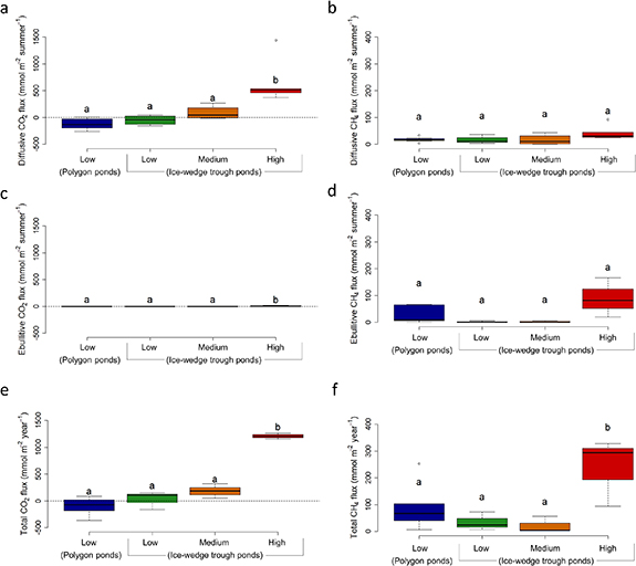
Figure 3. Greenhouse gas fluxes from ponds grouped by their level of erosion: low, medium, or high. The polygon pond group here include coalescent polygon ponds. Diffusive (a), (b) and ebullitive (c), (d) fluxes during stratified summer period (July and early August) are presented separately from total annual fluxes (e), (f), which include GHG emitted during ice-out (June) and autumnal mixing (late-August, September) periods. CO2 fluxes are shown on the left column, while CH4 fluxes are on the right side. Significantly different groups are indicated with letters above the boxplots. The dotted lines in graphs a and e separate the uptake from atmosphere (negative values) from emissions (positive values).
Download figure:
Standard image High-resolution imageRadiocarbon and 13C signatures of collected GHG and surface water DOC showed a differentiation depending on pond morphology and shore erosion intensity. In figure 4, we juxtaposed the radiocarbon age of GHGs and DOC with that of potential carbon sources. Dissolved and ebullition CH4 showed the clearest differentiation along the erosion gradient. Ponds with low erosion emitted the most modern carbon, while gases emitted from highly erosive ponds had a more 14C-depleted signature. The latter matched the age of peat stored in the active layer, while ponds with low or medium erosion better matched with modern carbon sources, here attributed to aquatic and terrestrial primary producers (e.g. benthic cyanobacterial mats, graminoids, and shrubs like Salix arctica).

Figure 4. Graphical summary of radiocarbon (14C) data for DOC and greenhouse gases. Signatures of surrounding carbon pools as potential carbon sources are indicated on the right side (see table S3; bent. = benthic mat, including cyanobacteria and brown mosses; atm. = atmosphere; veget. = graminoids and other plants growing near ponds; AL = soil organic matter from the top 35 cm of the active layer. The two data points older than the AL are likely respired from deepened active layer underlying ponds. Data points are coloured following the pond groups along the erosional gradient, from low (blue) and medium (orange) to high erosion (red). The low erosion group here is represented only by coalescent polygon ponds, as no isotopic data was available for low erosion ice-wedge trough ponds.
Download figure:
Standard image High-resolution imageThe trend along the erosion gradient was less clear for DOC and CO2 signatures (figure 4). To better explore the potential contribution of different carbon sources to CO2, we applied a Bayesian mixing model using both radiocarbon and 13C isotopes (figure 5). Dissolved and ebullition CO2 data were combined, as their signatures were not significantly different. The atmosphere was found to be the dominant source of CO2 in all studied ponds (45%–70%), with an important addition attributed to benthic producers (∼25% and 45% in low and medium erosion ponds respectively). Littoral vegetation appeared as an important contributor in medium erosion IWT ponds (10%), whereas other two groups had a similar contribution from methanotrophy. Only high erosion IWT ponds showed a significant contribution from carbon stored in the peat (active layer ∼20% and permafrost ∼5%).

Figure 5. Graphs illustrating the input (a) and output of a Bayesian mixing model demonstrating carbon sources for CO2 for the studied pond groups (b)–(d). CO2 data pool is differentiated by colour (a), blue circles denoting CO2 sampled in low erosion coalescent polygon ponds, orange triangles in medium erosion IWT ponds, and red triangles in high erosion IWT ponds. Carbon sources (bent. = benthic mat, including cyanobacteria and brown mosses; atm. = atmosphere; veget. = graminoids and other plants growing near ponds; AL = soil organic matter from the top 35 cm of the active layer, PMF = permafrost organic matter dated in soil collected between 40 and 100 cm depth, MO = methane oxidation, values from ebullition methane) are explained in more details in table S3.
Download figure:
Standard image High-resolution image
4. Discussion
This is the first study linking GHG emissions from tundra ponds with quantitative assessment of landscape disturbance due to permafrost thaw. Our data clearly show how permafrost degradation through shoreline erosion alters limnological properties of tundra ponds, creating conditions for greater production and accumulation of CO2 and CH4. Erosive IWT ponds emitted significantly more GHG than ponds with stable shores, on average by a factor of 6 for CO2 and 10 for CH4 (figure 3). This is when considering both diffusion and ebullition and including the component of GHG emitted in spring and autumn from winter and summer gas storage. The significant increases in bacterial FA (indicative of higher microbial biomass; Francisco et al 2016) and humic-like FDOM in high erosion ponds (figure 2(b)) indicate a larger influx of organic matter transformed by soil microorganisms (Stedmon and Cory 2014). In addition to bringing carbon and nutrients (notably phosphorus; table 1, figure S4(k)) to heterotrophic microbial communities, the influx of organic-rich soil particles likely affects the functional community itself, as demonstrated by Negandhi et al (2014), at the same site. Moreover, the influx of TSS and CDOM (figures 3 and S4) decreases the transparency of pond water, which together with unstable shores poses a serious hindrance to benthic and planktonic phototrophic communities, as demonstrated in boreal regions (Ask et al 2012). Therefore, eroding shores not only stimulate the production of high amounts of CO2, but also inhibit its consumption.
IWT ponds are narrow and hidden in depressions, reducing the impact of wind on the mixing regime of these water bodies (Prėskienis et al 2021). The underlying ice wedge (and the concentration of solutes by evaporation) likely further amplifies thermal stratification, which is present even in very shallow IWT ponds with negligeable erosion (30–40 cm deep; figure S4(a)). Combining the strong attenuation of light in the water column of humic ponds with the long sunny days of the Arctic summer, pond morphology can impede water column mixing during the summer, except for partial mixing that occurs on a daily basis (e.g. figure 4 in Bouchard et al 2015a). This generates conditions for a significant storage of GHG in the hypolimnion, which evade later during the autumnal turnover period, as seen for temperate lakes (Encinas Fernández et al 2014). When summer storage flux was included in the calculation (total fluxes; figures 3(e) and (f)), highly erosive IWT ponds were differentiated even further from other pond groups, as opposed to only comparing diffusive or ebullitive fluxes during the stratified summer period (figures 3(a)–(d)). Dissolved oxygen levels in these ponds were generally low at the surface (∼85% of atm. saturation), and particularly in the hypolimnion (<25% saturation). Oxygen depletion and constant inputs of carbon and nutrients from eroded peat blocks thus create favourable conditions for efficient CH4 production, as observed in other thermokarst systems (Matveev et al 2016, Serikova et al 2019). Since high erosion IWT ponds were stably stratified in July, most CH4 diffusing from the anoxic sediments accumulated in the hypolimnion, while bubbles could escape, explaining why higher diffusive CH4 fluxes were not concurrently observed with the higher ebullitive fluxes (figure 3). This result highlights the need to consider ebullitive and storage fluxes of CH4 when assessing the role of these water bodies on global GHG cycles.
Future estimates and extrapolations for larger areas are further complicated by the irregular frequency and severity of erosive events, as well as the heterogeneity of SOM (both in quantity and quality; Ping et al 2015, Zolkos and Tank 2020). Shore erosion often occurs on relatively large soil slabs (figures 1(h) and (i)) that can remain intact for long periods of time, limiting physical access of eroded SOM to pond microorganisms (Schmidt et al 2011). Although anecdotal, notable interannual fluctuations in ebullition fluxes were observed from erosive ponds at our study site, with substantial increases during the summer following a major erosion event, by 2–3 times as compared to the multiannual average (see table S6). By comparison, a thoroughly studied CP pond experienced only ∼10% interannual variations in its ebullition flux. Furthermore, the effects of permafrost disturbance on ponds can be temporary, as these processes can evolve very rapidly. Erosive IWT ponds are prone to infilling with collapsing soils (Kanevskiy et al 2017) or to stabilisation by vegetation succession (Jorgenson et al 2015). Expanding IWT ponds can also create drainage pathways and become dry troughs (Liljedahl et al 2016). Thus, over time, erosive shores can stabilise (a process observed at our study site over time), dry up completely, or expand into CP ponds or even lakes (Coulombe et al 2022). The length of this erosive stage is therefore critical in determining future GHG emissions from Arctic lowlands affected by permafrost thaw. While this study presents the general importance of erosion to GHG emissions, to better assess the importance of singular erosion events, more ponds need to be studied over a longer time period.
Ponds less affected by shore erosion (low to medium level) did not show significant differences in GHG emission rates (figure 3) or sources (figures 4 and 5) among themselves, despite the clear morphological and limnological differences (figures 1, 2 and S4 table 1). These ponds feature more transparent waters and stable shores, allowing the growth of benthic and planktonic phototrophic communities, including cyanobacterial mats (especially in CP ponds; figure 1(e)), brown mosses (omnipresent in low and medium erosion ponds), and aquatic plants (e.g. Eriophorum sp.). The different balance between respiration and photosynthesis likely explains the trend of increasing CO2 flux with the erosion level (figure 3(e)), while the reversed trend in CH4 flux (figure 3(f)) is potentially related to the temperature of the sediments (figure S4a, higher in polygon and CP ponds where heat is transported from the surface by constant mixing), as well as the efficiency of methanotrophy. Photosynthesising benthic mats provide methanogens with labile OM, measured here indirectly as fresh FDOM and polyunsaturated FAs, both of which were found more abundant in CP ponds, (figure 2(b)) while the well-lit water column possibly inhibits methanotrophs (as observed in boreal lakes; Thottathil et al 2018). Meanwhile, the more stable IWT ponds (low to medium level) had exceptionally low ebullition rates, possibly due to benthic vegetation dominated by brown mosses, which may physically obstruct rising CH4 bubbles, allowing more time for gas dissolution and promoting the activity of methanotrophic communities (Liebner et al 2011). Our mixing model, however, was unsuited to demonstrate this process, as methanotrophy did not appear as a particularly large carbon contributor for CO2 in the ponds (figure 5). Overall, benthic mats in shallow ponds are a critical component of Arctic ecosystems; further studies including fine vertical profiles of dissolved GHGs and their isotopic signature within the mats are needed.
With longer, warmer, and wetter summers, many tundra areas (both dry land and ponds) are becoming greener (Arndt et al 2019, Ayala-Borda et al 2021). This could lead to an overall larger CO2 sink on the landscape; however, CH4 emissions at the landscape scale may increase or decrease, depending on which ponds develop the most. We must also determine to which extent methanotrophic communities will thrive under future changes, and which pool of carbon (modern carbon from living biomass, or old carbon from permafrost) will dominantly contribute to methanogenesis. Warmer and snowier winters are expected to intensify shoreline erosion due to snow insulation and thermo-erosion by meltwater (Hinkel and Hurd 2006, Osterkamp et al 2009), which would hinder photosynthesis (higher CDOM, suspended solids, unstable shores), stimulate heterotrophic activity (Moquin and Wrona 2015), and with less benthic vegetation potentially limit the degree of methanotrophy. These diverging trajectories must be considered when assessing future GHG emissions from tundra landscapes, as local topography, permafrost properties, and regional climate trends can significantly alter the outcome.
5. Conclusions
Our results demonstrate that even small-scale abrupt disturbances of organic-rich permafrost can significantly affect GHG fluxes from shallow tundra ponds. IWT ponds with unstable shores emitted on average 6 times more CO2 and 10 times more CH4 than their counterparts with otherwise similar morphology, while CP and polygon ponds emitted relatively small amounts of CH4 and were small sinks of atmospheric CO2. With the intensification of soil erosion in permafrost regions, ponds are expected to become larger GHG emitters and should be considered as potential hotspots for permafrost carbon mineralisation.
Despite the dominantly modern radiocarbon signature of emitted GHG, ponds with intensely eroding shorelines show greater metabolism of carbon stored in the soil for centuries. Increased permafrost erosion in the future could thus lead to excess emissions of terrestrial carbon to the atmosphere at the ecosystem scale. Although small and shallow, these water bodies are numerous and occupy large areas in Arctic lowlands. Furthermore, their combined surface area is expected to expand with increasing permafrost temperatures and precipitation. If primary producers are unable to overcome the challenges of permafrost disturbance, GHG production and emissions from old carbon stocks could become more significant. A better understanding of pond-soil interactions and plant colonisation are essential to estimate the respective contribution of these highly differentiated carbon sources more accurately in the global carbon-climate system. We also must define more precisely the timeframe of the morphological evolution of tundra ponds, especially the duration of the erosive period.
Acknowledgments
We wish to thank Parks Canada, the Centre for Northern Studies (CEN) and G Gauthier for helping with logistics during fieldwork. We also thank A Veillette, F Bouchard, and V Laderriere for their assistance with collecting and processing the samples, and X Xu and M F Billett for their contribution on 14C analyses. We further extend our acknowledgements to T Pacoureau and F Mazoyer for their most valuable assistance in collecting samples and interpreting the results. The study was funded by the Natural Sciences and Engineering Research Council Discovery program, Network of Centres of Excellence ArcticNet, Natural Resources Canada Polar Continental Shelf Program, International Polar Year, and Fonds de recherche du Québec—Nature et technologies (IL), as well as the CREATE program EnviroNorth (VP).
Data availability statement
All data that support the findings of this study are included within the article (and any supplementary files).
The raw data can also be found in Nordicana D data repository (Prėskienis et al 2023).
Author contribution
VP, DF, and IL were involved in study planning and data collection in the field. VP carried out the data analysis, produced the figures, and drafted the manuscript under the supervision of IL and DF. PD and MR contributed their expertise to the analysis and interpretation of isotope (PD) or fatty acid (MR) data. All authors contributed to the revision of the manuscript.
Supplementary data (3.4 MB DOCX)