

Abstract
Signatories to the Paris Agreement have pledged to keep global warming to well below 2 °C above pre-industrial levels and preferably below 1.5 °C above pre-industrial levels. Beyond over-shooting Paris Agreement warming levels followed by net negative emissions, achieving a state of net zero carbon dioxide emissions is required to satisfy Paris Agreement warming goals. Research on climate changes under net zero CO2 emissions is very limited to date with no comprehensive analysis of changes in extremes. In this study, we use results from Earth System Models in the zero emissions commitment model intercomparison project to understand regional mean-state climate change patterns during a 100 year period following carbon dioxide emissions cessation. We also perform an initial study of the evolution of hot and cold monthly temperature extremes after net zero CO2 emissions, including an assessment of how the change in frequency of temperature extremes affects areas of different levels of socioeconomic development based on regional Human Development Index (HDI). The results show that most land regions experience a fast and continuous cooling response following emissions cessation, with large areas of significant model agreement. In contrast, the Southern Ocean continues warming over the century after emissions cessation. The frequency of land-based local monthly high temperature extremes generally stays constant or decreases during the century after emissions cessation, however, decreases in heat extreme frequencies are generally less for locations with lower modern HDI than areas with higher HDI which suggests that inequality of climate change will remain an issue even after net zero CO2 emissions. There is an evident emergence of local monthly cold extremes following emissions cessation with most significant impact over high HDI mid- and high-latitude land regions.
Export citation and abstract BibTeX RIS

Original content from this work may be used under the terms of the Creative Commons Attribution 4.0 license. Any further distribution of this work must maintain attribution to the author(s) and the title of the work, journal citation and DOI.
1. Introduction
The Intergovernmental Panel on Climate Change has assessed the current state of the global climate concluding that human-caused climate change has caused warming on land, within the ocean, and in Earth's atmosphere, with a likely global mean surface temperature increase from 1850–1900–2010–2019 of 0.8 °C–1.3 °C attributed to human influence (IPCC 2021). Anthropogenic climate change also has a proven impact on weather and climate extreme events, with virtual certainty that both frequency and intensity of heat extremes have increased since the mid-twentieth century because of human-caused climate change (IPCC 2021). In response to the observed effects of climate change, the Paris Agreement was agreed to in 2015 with the core goal of limiting the increase in global-average temperature to well below 2 °C above pre-industrial levels and pursuing efforts to limit the temperature increase to 1.5 °C above pre-industrial levels. From a geophysical science perspective, there is a requirement to reach at least net-zero CO2 to limit human-induced global warming, along with reductions of other greenhouse gases (IPCC 2021). In a state of net zero CO2 emissions, residual anthropogenic CO2 emissions are balanced by anthropogenic negative emissions.
There have been several studies that have investigated climate response to reaching a state of net zero using state-of-the-art climate model simulations (Matthews and Caldeira 2008, Plattner et al 2008, Frölicher and Joos 2010, Gillett et al 2011, Zickfeld et al 2013, MacDougall et al 2020, Jenkins et al 2022). The most relevant studies to this research use the Zero Emissions Commitment Model Intercomparison Project (ZECMIP), which includes a collection of Earth System Models (ESMs) and ESMs of Intermediate Complexity (EMICs) configured in emissions-driven mode, where the carbon dioxide atmospheric concentration and downstream climate impacts are determined based on the model representations of the carbon cycle, as opposed to concentration-driven modeling where the atmospheric carbon dioxide concentration is prescribed. More information regarding the emissions driven configuration used in ZECMIP experiments can be found in Jones et al (2016).
MacDougall et al (2020), used the collection of ESMs and EMICs in ZECMIP (Jones et al 2019) to simulate heat and carbon redistribution and committed global warming following emission cessation. The simulations are initially run using a 1% per annum increase in CO2 concentrations until specific diagnosed cumulative emissions are reached (750 PgC, 1000 PgC, and 2000 PgC), at which point emissions are set to zero and models freely evolve in an emissions-driven configuration; the initial 1% CO2 per annum can be in either concentration-driven or emissions-driven mode depending on modeling agencies ability to avoid introducing shock to the model system when changing to the zero emissions phase of the experiment (Jones et al 2019). The ZEC, which is defined as the change in global mean surface temperature following a complete cessation of carbon dioxide emissions, has become a well-used metric. Researchers have analyzed ZEC on various timescales, but ZEC is now commonly analyzed over multi-decadal timescales which are more relevant for policymakers. MacDougall et al (2020) found that, following carbon dioxide emissions cessation, there was a rapid reduction in atmospheric CO2 concentrations followed by a decreasing rate of decline, consistent with several other studies (Frölicher and Joos 2010, Gillett et al 2011). Additionally, MacDougall et al (2020) found that ZEC is most likely near zero on multi-decadal timescales, which is consistent with previous model experiments using EMICs (Plattner et al 2008) and emission driven ESMs of full complexity (Lowe et al 2009, Frölicher and Joos 2010, Gillett et al 2011).
In a more recent study MacDougall et al (2022) investigate multi-decadal regional scale committed warming patterns following CO2 emissions cessation. ZEC is computed on a regional basis to better understand regional temperature variation following a complete cessation of carbon dioxide emissions. The authors find significant differences regionally in both the sign and magnitude of ZEC. For nearly all ESMs included in the study, there is cooling over both land and ocean on average, with a warming lag period immediately after emissions cessation. For most ESMs, there is large scale cooling over land globally, and most models show cooling trends over ocean regions, however with some models disagreeing on warming/cooling signs in multiple oceanic regions throughout the domain; large differences in land-ocean response are consistent with previous modeling studies of various types of experimental designs (Joshi et al 2008, Rugenstein et al 2019, King et al 2020).
Overall, research has shown a carbon redistribution between land, ocean, and atmosphere following emissions cessation, resulting in falling atmospheric CO2 concentration (e.g. MacDougall et al 2020). Overall rates of land and ocean uptake of atmospheric CO2 are key components in determining global surface temperature response after CO2 emissions cessation MacDougall et al (2020). Global committed warming is projected to be near zero, however regional warming commitments can be significant with large uncertainty between current available models. The committed climate changes have been shown to depend on the cumulative carbon emissions at the time of emissions cessation.
While previous studies have explored global responses to net zero emissions, limited work has focused on connecting global-scale climate change to regional climate. Further research regarding regional climate change following net zero CO2 emissions is important because achieving a stable global mean temperature within Paris Agreement goals is not the same as achieving stable climate in individual regions; further research can help build an understanding of regional changes and nuances post net zero CO2 emissions. In addition, although many studies have considered changes in climate extremes using scenarios that reach periods of net zero CO2 emissions (such as SSP1-1.9 and SSP1-2.6), analysis of temperature extremes using idealized net zero climate model experiments like ZECMIP has not been conducted. In this study, we address existing research gaps by, first, identifying robust regional warming and cooling patterns following a complete cessation of carbon dioxide emissions. Second, we present an analysis of how the frequency of regional hot and cold monthly temperature extremes change following emissions cessation in the ZECMIP ensemble. Third, we investigate how changes in temperature extremes following net zero impact regions of varying socioeconomic development quantified using the Human Development Index (HDI).
2. Data and methods
2.1. The ZECMIP
The ZECMIP, a sub-project of CMIP6 (Eyring et al 2016), was designed to quantify temperature change following a complete cessation of CO2 emissions (i.e. the ZEC), and to investigate the geophysical drivers behind the climate response to CO2 emissions cessation (Jones et al 2019). Note, ZEC can be evaluated from emissions cessation of only CO2 (MacDougall et al 2020), non-CO2 gases such as CH4 or N2O (Matthews and Zickfeld 2012), or all anthropogenic emissions (Hare and Meinshausen 2006). However, on decadal timescales, ZEC from ceasing emission of all forcing agents tends to converge to ZEC values from cessation of only CO2 emissions which makes ZECMIP a reasonable choice given the simulation lengths of participating ESMs.
In this work, ZECMIP experiment esm-1pct-brch-1000 PgC (called experiment A1 from hereon) was used, which corresponds to about 2 °C CO2-induced warming relative to pre-industrial (Jones et al 2019). Experiment A1 sets CO2 emissions to zero once cumulative CO2 emissions reach 1000 PgC, after which models are allowed to freely evolve for at least 100 years. Table S1 shows the ESMs included in the analysis with expanded model descriptions available in Table A1 of MacDougall et al (2020); note, GFDL-ESM2M was the original submission to ZECMIP but has since been replaced by results from GFDL-ESM4. The models included in this analysis are the nine that were available on the Earth System Grid Federation Australian node as of January 2022.
2.2. Global and regional ZEC
ZEC is defined as the change in global temperature projected to occur following a complete cessation of CO2 emissions (Matthews and Weaver 2010, MacDougall et al
2020). In this report, ZEC is quantified over multi-decadal intervals on a global average and an individual grid level (latitude–longitude) basis. Figure 1 shows a simple schematic which illustrates how ZEC is quantified using data from the MIROC-ES2L model as an example. In figure 1, the 1pctCO2 portion of the experiment is represented by the blue curve, which is initialized at the pre-industrial condition for each model. The red curve represents the temperature evolution following a complete cessation of carbon dioxide emissions, which occurs at time  in figure 1. The near-surface air temperature (tas) variable is used.
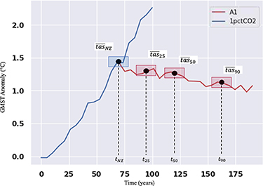
Figure 1. Illustration of baseline and ZEC climatologies (centered about years 25, 50, and 90 after emissions cessation) used to compute global and regional ZEC values. The red shaded boxes illustrate the 20 year time frames used for the ZEC climatologies and the blue shaded box illustrates the 20 year time frame used for the baseline net zero climatology. Note, the baseline net zero climatology uses only data from the 1pctCO2 curve.
Download figure:
Standard image High-resolution imageThe CMIP variable for near surface air temperature (tas) is used for all temperature calculations. For each model in the ensemble, the baseline net zero climatology,  from figure 1, is computed using a 20 year window centered at the time of branching denoted
  ; the 20 year baseline climatology is computed as the mean climate bounded by upper and lower bounds illustrated by the blue shaded time frame along the 1pctCO2 curve in figure 1. Once the baseline climatology is known, global ZEC time series are then computed for each model using equation (1):

where  is the time series representing the difference in global mean surface temperature evaluated at time
  and the baseline climatology
  . Figures S1 and S2 in the supplementary information show the global mean surface temperature anomalies and global ZEC time series for the nine ESMs, respectively. Comparable ZEC time series can be found in MacDougall et al (2020) figure 2(b).
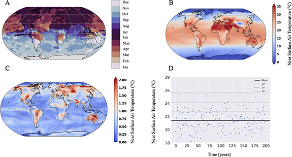
Figure 2. Using MIROC-ES2L pre-industrial control, (A) distribution of months associated with maximum local near surface air temperatures. (B) Mean near surface air temperature distribution from pre-industrial control associated with local maximum month. (C) Standard deviation distribution of near surface air temperatures from pre-industrial control associated with local maximum month. (D) Pre-industrial control mean near-surface air temperature and computed extreme levels  –
– for grid cell over Melbourne, Australia.
Download figure:
Standard image High-resolution imageTo compute regional changes in ZEC, 20 year climatologies are computed for three unique time periods following emissions cessation. In this research, 20 year climatologies are centered at 25, 50, and 90 years after emissions cessation, consistent with previous research (MacDougall et al
2020, 2022). The three ZEC time frames are centered about  ,
,  , and
, and  , respectively as shown in figure 1; the three ZEC time frames are illustrated by the red shaded portions of the net zero CO2 portion (red curve) shown in figure 1. Regional (lat, lon) distributions of ZEC for each ZEC time window (ZEC25, ZEC50, ZEC90) are then computed using equation (2):

where  is the near-surface air temperature at each grid point (lat, lon) averaged over a 20 year window centered at the year defined by subscript Y (subscripted years include 25, 50, and 90).
  is the baseline climatology defined as an averaged 20 year window centered at the time associated with the net zero branch,
  . Figure S3 shows baseline climatologies for each of the nine participating ESMs. Equation (2) is applied for each model within the ensemble (n = 9). Figures S4–S6 show the spatial distribution of ZEC25, ZEC50, and ZEC90 for the nine models included in the ensemble, respectively. As highlighted in MacDougall et al (2022), there are significant differences in regional projections of ZEC especially in high-latitudes. The significant differences in regional ZEC projections are noteworthy when considering ensemble mean results, especially in areas such as Arctic latitudes where the largest spread between the models in the ensemble exists.
2.3. Local monthly temperature extremes
We assess how high temperature extreme events will evolve after net zero carbon dioxide emissions are achieved by investigating how temperatures during location-specific hottest months change after CO2 emissions cessation. Local monthly hot temperature extreme thresholds are calculated using the means and standard deviations of the local monthly maximum temperature determined from the pre-industrial control simulation. Monthly temperature data was used so that all nine models could be included in the analysis. Similar methods have been used to study the historical precedence of the 2021 Pacific Northwest heatwave (Neal et al 2022). To compute extreme thresholds for local monthly maximum temperature extremes, first, the calendar month associated with local maximum monthly temperature was determined for each model using the pre-industrial control runs. Figure 2(A) shows a map with the distribution of months associated with maximum near surface air temperature using the MIROC-ES2L model as an example. Maps of the month associated with maximum temperature were also created for the other models and can be found in figure S7.
After determining the month associated with monthly maximum temperature for each grid cell, ensemble means and standard deviations ( ) are computed for each grid cell's month of maximum temperature. Distributions of mean and standard deviation of local monthly maximum temperature from the piControl simulation are shown in figures 2(B) and (C), respectively. Peak mean temperatures are primarily located over tropical and mid latitude land surfaces. Standard deviation, which is indicative of natural variability in the unforced pre-industrial control experiment, is largest over land surfaces, with generally lower variability in the tropical latitudes. Thresholds of local monthly temperature extrema are then computed for each standard deviation level (
 -level) using equation (3):
where  represents monthly extreme temperature distribution at a given
  -level,
 represents the local (lat, lon) mean near surface air temperature for the month of maximum temperature, and
  is the standard deviation of local (lat, lon) monthly maximum temperature. In the standard deviation term (second term, right hand side), the multiplier
  is used to compute specific
  -level extreme thresholds. For this research,
  through
  extreme thresholds are considered for hot temperature extremes (
 = 1, 2, or 3). As an example of a grid-based extreme temperature calculation, figure 2(D) depicts the mean and extreme thresholds
  –
– for the closest grid cell over Melbourne, Australia (38° S, 144° E) using the MIROC-ES2L model. The data is specific to the pre-industrial control simulation restricted to the local month of maximum temperature (computed as February over Melbourne for the MIROC-ES2L ESM).
Frequencies of local (lat, lon) monthly hot temperature extreme exceedance are computed for the net zero baseline climatology (20 year window centered at the time of branching denoted  from figure 1), and for the ZEC25 and ZEC90 20 year windows. The frequencies of monthly temperature extremes for the 20 year ZEC time frames and the 20 year baseline climatology express the percentage of years (out of 20) that a local grid cell exceeds local
  -level thresholds. Changes in frequency of local monthly hot temperature extremes are computed for the ZEC25 and ZEC90 20 year time frames using equations (4) and (5):


where  and
and  are local (lat, lon) frequencies of
  -level (N = 1, 2, or 3) monthly temperature extremes for the ZEC25 and ZEC90 20 year time windows, respectively.
  represents local (lat, lon) frequencies of
  -level (N = 1, 2, or 3) monthly temperature extremes for the 20 year net zero baseline climatology (centered at tNZ from figure 1). Differences in extreme frequency over the century after emissions cessation are computed by subtracting the frequencies during the ZEC90 time window by frequencies during the ZEC25 time window.
Changes in local monthly cold extremes were also investigated. The methodology for defining cold extremes follows a similar approach as determining hot extremes, however for cold extremes, the  -level thresholds are based on local minimum monthly temperatures determined for each grid cell. Additionally, extreme thresholds are computed using −0.25
 , −0.5
 , and −1
 for cold extremes because comparable thresholds to those used for the hot extremes analysis are rarely achieved after the simulated warming from the 1pctCO2 phase of the idealized experiment. Changes at these
  -levels are not always considered as extreme, however trends in −0.25
 , −0.5
 , and −1
 sigma level events will suggest changes in frequency of 'colder-than-average' cold months following net zero. Additionally, although the extreme level thresholds used for cold extremes here are less than thresholds used for heat extremes, cold extreme events at
  thresholds can cause damage and are still studied in current research (Dai et al
2021). For consistency with the local monthly hot extreme convention used in this research, we refer to changes in cold month frequencies as 'cold extremes' throughout the paper. The supplemental material includes an analysis and illustration that shows the method for computing local monthly cold extreme thresholds using a similar approach to the local monthly heat extreme analysis captured in figure 2. Figure S8 in the supplementary material shows the distribution of local coldest months for the nine ESMs. Using the MIROC-ES2L ESM as an illustrative example, figure S9 in the supplementary material shows distribution of months associated with minimum local near surface air temperatures, mean near surface air temperature distribution from pre-industrial control associated with local minimum month, standard deviation distribution of near surface air temperatures from pre-industrial control associated with local minimum month, and pre-industrial control mean near surface air temperature and computed extreme levels—
thresholds can cause damage and are still studied in current research (Dai et al
2021). For consistency with the local monthly hot extreme convention used in this research, we refer to changes in cold month frequencies as 'cold extremes' throughout the paper. The supplemental material includes an analysis and illustration that shows the method for computing local monthly cold extreme thresholds using a similar approach to the local monthly heat extreme analysis captured in figure 2. Figure S8 in the supplementary material shows the distribution of local coldest months for the nine ESMs. Using the MIROC-ES2L ESM as an illustrative example, figure S9 in the supplementary material shows distribution of months associated with minimum local near surface air temperatures, mean near surface air temperature distribution from pre-industrial control associated with local minimum month, standard deviation distribution of near surface air temperatures from pre-industrial control associated with local minimum month, and pre-industrial control mean near surface air temperature and computed extreme levels— through −
 for grid cell over Melbourne, Australia.
2.4. Local monthly hot and cold extremes and the HDI
Less economically developed regions experience disproportionate loss and damage from climate extremes such as heatwaves, floods, and tropical storms (Gamble et al 2016, Birkmann et al 2022) To improve understanding of how the frequency of temperature extremes might affect populations with different levels of vulnerability following CO2 emissions cessation, the relationship between local monthly maximum temperature extremes and local HDI was explored. HDI is a unique multidimensional measure of development and serves as an important alternative to some traditional single dimensional measures of development such as gross domestic product (Sagar and Najam 1998). HDI is a composite measure that considers length and health of life, access to education, and standard of living (Kummu et al 2018). HDI was chosen for this study as a measure of socioeconomic development because the HDI includes social indicators as well as economic development. Figure S10 shows the 2015 HDI distribution used in this study. HDI changes over time due to developments such as improvements in regional economic markets, increased access to healthcare, and advancements in local education. However, projections of HDI have not been developed in accordance with the CO2 emissions cessation scenario used under the ZECMIP framework. Therefore, static regional HDI values based on the recent 2015 dataset from Kummu et al (2018) are used here. The HDI dataset from Kummu et al (2018) has been used in other studies examining inequality of climate change impacts (e.g. Lieber et al 2022).
3. Results
3.1. Regional ZEC
To provide a comprehensive projection of how ZEC varies spatially within the ensemble, median ZEC distributions for ZEC25 and ZEC90 time windows are shown in figures 3(A) and (B), respectively. The median was chosen here to avoid skewing regional results from the limited sample size (n = 9) towards outliers such as the CESM2 model which shows a strong inter-hemispheric temperature gradient after CO2 emissions cessation. The inter-hemispheric relationship exhibited by CESM2 is shown in the supplemental material Figures S4–S6, and is also shown in figure 3 of MacDougall et al (2022). Additionally, to evaluate the change in ZEC over the century following carbon dioxide emissions cessation, the regional difference between median ZEC90 and ZEC25 was computed and is shown in figure 3(C). If at least eight of the nine ESMs show agreement in the sign of ZEC (or sign of change in ZEC in the case of figure 3(C)) then this corresponds to p-value <0.05 (calculated using the binomial distribution) and is taken to be statistically significant. Figure S13 in the supplemental material shows an illustration of the fundamental binomial distribution with a nine-model sample size. Although ESMs are not entirely independent (Knutti et al 2013), the ESMs participating in ZECMIP have a large diversity of component sub models as shown in tables A1 and A2 from MacDougall et al (2020).
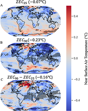
Figure 3. Ensemble median of (A) ZEC25 regional distribution and (B) ZEC90 regional distribution, and (C) difference between ZEC90 and ZEC25 distributions. In (A) and (B), cross-hatching indicates that at least 8 ESMs have the same sign of ZEC locally. In (C), cross-hatching indicates that at least 8 ESMs show same sign of change in ZEC from ZEC25 to ZEC90. Ensemble medians of global mean values of ZEC25, ZEC90, and the difference between ZEC90 and ZEC25 are in parenthesis of titles of (A)–(C) respectively.
Download figure:
Standard image High-resolution imageThe ZEC distributions show cooling or warming responses between −0.5 °C and 0.5 °C with significant regional variation consistent with previous work from MacDougall et al (2022). The global mean surface temperature decline 0.07 °C by the ZEC25 time frame and continues to decline an additional 0.14 °C over the century after CO2 emissions cessation. An ensemble median global mean surface temperature drop of 0.16 °C over the century after CO2 cessation is noteworthy considering the scale of global surface temperature goals established in the Paris Agreement (<2 °C above pre-industrial levels with efforts to limit to 1.5 °C). The model-specific global ZEC results are available in table S1 in the supplementary material. The regional ZEC distributions show a rapid cooling response over land with continued cooling as the ZEC time window reaches ZEC90, with the largest land surface cooling occurring in the Northern Hemisphere. The largest warming is projected in the northeast Pacific Ocean, and Southern and Indian Ocean roughly between longitudes 70° W (Cape Horn, Chile) and 175° E (New Zealand). Overall, land exhibits greater cooling than the ocean likely because of differences in oceanic and land heat capacities, where land show quicker recovery to pre-industrial temperatures than ocean areas (MacDougall et al 2022). It is also possible that changes in local feedbacks and the hydrological cycle causes greater cooling over land than the ocean (Joshi et al 2008). There is an initial cooling by ZEC25 followed by a rebound in near-surface air temperature over the century after ZEC25 in the North Atlantic. This is possibly due to the evolution of Atlantic Meridional Overturning Circulation projected by the models; results from MacDougall et al (2022) suggest diverse evolution of AMOC between the models with some models showing an AMOC strengthening by the end of the century after CO2 emissions cessation.
The ESMs show significant agreement of cooling over land, with increasing area of the planetary surface having significant model agreement by the ZEC90 time frame. There is also significant model agreement of cooling in tropical Atlantic, Indian, and western Pacific Oceans seen in the ZEC90 figure 3(B); this strong cooling agreement is driven by continued temperature changes between ZEC90 and ZEC25 as captured by the cross-hatching in figure 3(C). There is significant warming agreement within the ensemble shown as a sharp band of warm sea surface temperatures in the Southern and Indian Oceans spanning between longitudes 70° W–175° E in the ZEC25 and ZEC90 time windows. The continued warming in the Southern Ocean after CO2 emissions cessation is possibly due to delayed circumpolar upwelling and equatorward transport (Armour et al 2016). In terms of continued warming between ZEC25 and ZEC90 time frames (figure 3(C)), there is negligible warming agreement between the ESMs in the ensemble. Figure S11 in the supplementary material includes mean ZEC distributions, the additional ZEC50 time frame, and shows the ensemble spread in ZEC for each time window. There is significant spread of ZEC values regionally with the highest spread located in high latitudes quite possibly due to different model representations related to AMOC and sea-ice coverage (MacDougall et al 2022).
Most participating ESMs ran a single ensemble member for the ZECMIP A1 experiment, however two of the nine ESMs ran the experiment with three members (UKESM1-0-LL and CanESM5). As an additional analysis, ZEC regional distributions of the two models with multiple ensemble members were examined to understand how variability within the models compare to mean changes in regional ZEC25 and ZEC90 patterns. Figures S15 and S19 show regional ZEC projections for each model member (n = 3) for CanESM5 and UKESM1-0-LL, respectively. For the CanESM5 data, the three simulations tend to show large land areas with ZEC positive/negative sign agreement during the ZEC90 time frame, but less so in the ZEC25 time frame. The UKESM1-0-LL members show large areas of ZEC positive/negative sign agreement for both ZEC25 and ZEC90 time frames. Further investigation is needed to determine more accurate projections of regional ZEC using larger sets of multi-member ensembles than are currently available.
3.2. Local monthly heat extremes
Once  through
  local monthly temperature extreme thresholds were computed for each model in the ensemble using methods described in section 2.3, changes in frequencies of local maximum monthly temperature extreme exceedances were computed using the 20 year ZEC25 and ZEC90 time frames using equations (4) and (5). Figure 4 shows frequencies of
  through
  local monthly heat extremes during the net zero baseline climatology, the changes in frequencies of
  through
  local monthly heat extremes during the ZEC25 and ZEC90 time frames, and the change in frequency between ZEC90 and ZEC25 time frames.
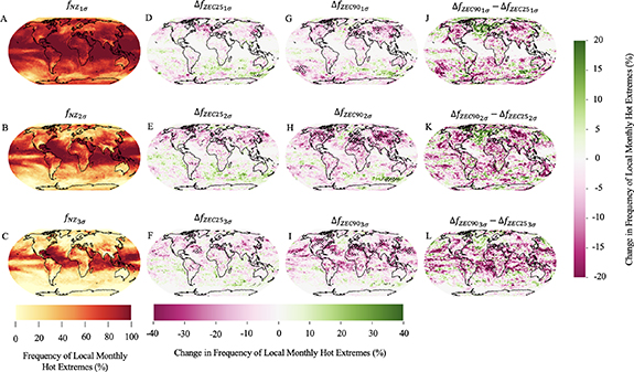
Figure 4. Ensemble median frequency (N years out of 20 expressed as a percentage) of 1 through 3
 local hot monthly temperature extremes in 20 year net zero baseline climatology (A)–(C). Ensemble median change in frequency (N years out of 20 expressed as a percentage) of 1
  through 3
  local hot monthly temperature extremes in ZEC25 (DEF) and ZEC90 (G)–(I) 20 year time frames. Changes in frequency of local hot monthly temperature extremes for −1
 through 3
 extreme levels, evaluated as the ZEC90 frequency distribution subtracted by the ZEC25 frequency distribution (J)–(L). Note, the colorbar below the first column correspond to maps (A)–(C), the colorbar below the two middle columns correspond to maps (D)–(I), and the colorbar on the right side of the grid of maps corresponds to maps (J)–(L). Cross-hatching in (D)–(I) indicates that at least 8 models show sign agreement of change in frequency of local hot monthly temperature extremes relative the frequencies from the 1pctCO2 net zero baseline climatology. Cross-hatching in (J)–(L) indicates at least 8 models show sign agreement of change in frequency of local hot monthly extremes over the century after emissions cessation evaluated as ZEC90 minus ZEC25 frequencies.
Download figure:
Standard image High-resolution imageDuring the 20 year net zero baseline time frame, land-based grids exhibit very high frequency of local monthly heat extremes for the 1 threshold. For 2
 and 3
and 3 thresholds, highest frequencies of local monthly heat extreme exceedances during the net zero baseline climate time frame are largely shown in tropical latitudes due to low variability in the tropics (Hawkins et al
2020, Mahlstein et al
2011). When the ZEC25 time frame is reached, most land surfaces exhibit either no change or a large-scale initial decline in frequency of local monthly heat extreme following CO2 emissions cessation with some exceptions such as areas of Northern Asia and midwestern North America. In the ZEC25 time frame, there are greater decreases in frequencies of land-based monthly heat extremes for 2
thresholds, highest frequencies of local monthly heat extreme exceedances during the net zero baseline climate time frame are largely shown in tropical latitudes due to low variability in the tropics (Hawkins et al
2020, Mahlstein et al
2011). When the ZEC25 time frame is reached, most land surfaces exhibit either no change or a large-scale initial decline in frequency of local monthly heat extreme following CO2 emissions cessation with some exceptions such as areas of Northern Asia and midwestern North America. In the ZEC25 time frame, there are greater decreases in frequencies of land-based monthly heat extremes for 2 and 3
and 3 thresholds than the decreases in frequencies for the 1
 threshold, especially in tropical latitudes. Although land-based initial reductions in frequency of local monthly heat extremes (especially for 2
 and 3
and 3 thresholds) are evident in many regions, the areas of largest initial decline in frequency of local monthly heat extreme frequency are over land in the Northern Hemisphere. While frequencies of land-based extremes tend to decline during the ZEC25 time frame, large oceanic regions have a projected increase in frequency of local monthly heat extremes after CO2 emissions cessation; specifically, the South Atlantic, Indian Ocean, and Southern Ocean have areas where frequency of local monthly heat extremes are projected to increase with significant model agreement south of Australia. The pattern of increasing oceanic frequencies in the Southern Hemisphere resembles changes in regional ZEC25 shown in figure 3(A).
By the ZEC90 time frame, there are widespread reductions in frequency of 2 and 3
and 3 local monthly heat extreme with the largest frequency reductions over land in the Northern Hemisphere. For each extreme threshold, areas of model significance emerge in the ZEC90 time frame over land in the Northern Hemisphere. Changes in local monthly heat extreme frequencies during the ZEC25 and ZEC90 time frames closely follow the mean state regional ZEC90 patterns (figure 3(B)) where large-scale land cooling is accompanied by warming in the Southern and Indian Ocean south of Australia.
There are continued reductions in land-based local monthly heat extreme frequencies for the remainder of the century after ZEC25 shown in figures 4(J)–(l). These continued reductions in local monthly heat extreme frequencies resemble the land response in near-surface air temperature shown in figure 3(C). Despite large land regions showing reductions in heat extreme frequency, there are virtually no areas with significant model agreement. After a small initial decline in frequency of local monthly heat extremes in the northern North Atlantic (especially for 1 and 2
and 2 ), heat extremes in the northern North Atlantic show a rebounding trend after ZEC25 time frame shown in figures 4(J)–(l). This northern North Atlantic rebounding trend is also evident in regional ZEC patterns in figure 3 which is possibly due to evolution in AMOC after CO2 emissions cessation.
Supplementary analysis was done to analyze regional patterns of local monthly heat extreme changes using the two participating ESMs with multiple simulation members (UKESM1-0-LL and CanESM5). Analysis for the two models was performed using identical methods as for the single member analysis discussed in the methods section, and results are found in supplementary information. The results show similar spatial patterns for extreme frequency changes between the three members of each model ensemble, however there are areas where the members show differences in sign changes of local monthly heat extremes; additional members for each ESM would help improve understanding of changes in heat extremes after CO2 emissions cessation.
3.3. Local monthly cold extremes
Once 0.25 –1
–1 local monthly cold temperature extreme thresholds were computed for each model in the ensemble, the change in frequencies of local minimum monthly temperature extreme exceedances were computed using the 20 year ZEC25 and ZEC90 time frames the same way as above for monthly warm extremes. Figure 5 shows the ensemble median frequencies of local monthly cold extremes, changes in frequencies of local monthly cold extremes after CO2 emissions cessation, and trends in frequency over the remainder of the century after ZEC25 computed as the difference in frequency during ZEC90 and ZEC25 time frames.

Figure 5. Ensemble median frequency (N years out of 20 expressed as a percentage) of −0.25 through −1
 local cold monthly temperature extremes in 20 year net zero baseline climatology (A)–(C). Ensemble median change in frequency (N years out of 20 expressed as a percentage) of −0.25
 through −1
 local cold monthly temperature extremes in ZEC25 (D)–(F) and ZEC90 (G)–(I) 20 year time frames. Changes in frequency of local cold monthly temperature extremes for −0.25
 through −1
 extreme levels, evaluated as the ZEC90 frequency distribution subtracted by the ZEC25 frequency distribution (J)–(L). Note, the colorbar below the first column correspond to maps (A)–(C), the colorbar below the two middle columns correspond to maps (D)–(I), and the colorbar on the right side of the grid of maps corresponds to maps (J)–(L). Cross-hatching in (D)–(I) indicates that at least 8 models show sign agreement of change in frequency of local cold monthly temperature extremes relative the frequencies from the 1pctCO2
net zero baseline climatology. Cross-hatching in (J)–(L) indicates at least 8 models show sign agreement of change in frequency of local cold monthly extremes over the century after emissions cessation evaluated as ZEC90 minus ZEC25 frequencies.
extreme levels, evaluated as the ZEC90 frequency distribution subtracted by the ZEC25 frequency distribution (J)–(L). Note, the colorbar below the first column correspond to maps (A)–(C), the colorbar below the two middle columns correspond to maps (D)–(I), and the colorbar on the right side of the grid of maps corresponds to maps (J)–(L). Cross-hatching in (D)–(I) indicates that at least 8 models show sign agreement of change in frequency of local cold monthly temperature extremes relative the frequencies from the 1pctCO2
net zero baseline climatology. Cross-hatching in (J)–(L) indicates at least 8 models show sign agreement of change in frequency of local cold monthly extremes over the century after emissions cessation evaluated as ZEC90 minus ZEC25 frequencies.
Download figure:
Standard image High-resolution imageThere are virtually no areas where local monthly cold extreme frequencies are elevated during the net zero baseline climatology because of large-scale warming prior to emissions cessation. Note, maps in figure 5 are based on ensemble medians of local cold monthly frequencies, however, there are areas that show slight increases in ensemble mean local cold monthly extremes during the net zero baseline climatology as shown in figure S14 of the supplemental material; these areas are clearest over high-latitude grids in the Atlantic Ocean possibly due to reduced meridional heat transport from weakening AMOC strength during the 1pctCO2 emissions phase of the experiments.
After CO2 emission cessation, local monthly cold temperature extremes become more frequent in many extratropical land areas. The most obvious signals are seen in the −0.25 and −0.5
 thresholds over North America, Europe, Northern Asia, Greenland, southern South America, Australia, and Antarctica. At the −1
 threshold, changes in frequency are very subtle with small frequency increases over Northern Hemisphere land, Antarctica, the northern North Atlantic, and the Southern Ocean; this is because, for all models, global mean temperatures exceed 1 °C warming relative to pre-industrial levels following the 1pctCO2 ramp-up phase of the experiment (see figure S1 in supplementary material). Areas with significant ensemble agreement (eight or more ESMs) of increased local monthly cold extreme frequency are clearest over Northern Hemisphere land, and over Antarctica for −0.25
 and −0.5
 threshold. There are negligible areas with significant ensemble agreement at the −1
 threshold because it is rare to exceed the 1
 threshold at elevated global mean temperature.
Over the remainder of the century after the ZEC25, there are large areas of increasing frequency of local monthly cold extremes, as high as 10%, which are again most evident in the mid-to-high latitudes in North America and northern Asia. There are also regions with reduction in frequency of cold extremes over the remainder of the century after ZEC25; for each  threshold, the northern North Atlantic ocean exhibits decreased frequency of local monthly cold extremes after the initial increased frequency shown in the ZEC25 time frame. Similar to frequencies of local monthly heat extremes, there are very limited areas of significant ensemble agreement (8 or more ESMs) of increasing or decreasing frequency of cold extremes over the remainder of the century after ZEC25.
3.4. Monthly temperature extremes and human development index
Figure 6 shows ensemble median frequency of local hot monthly temperature exceedance during net zero baseline climatology (A)–(C), ensemble median change in frequency of local hot monthly temperature extreme exceedance plotted against HDI for land-based grid cells for the ZEC25 (D)–(F), and ZEC90 (G)–(I) time frames and the difference between the two time frames (J)–(L).

Figure 6. Ensemble median monthly hot temperature extreme frequency in 20 year net zero baseline climatology (A)–(C) plotted against Human Development Index (HDI). Change in ensemble median monthly hot temperature extreme frequency in ZEC25 (D)–(F) and ZEC90 (G)–(I) windows plotted against Human Development Index. Marker sizes are based on population size, with a reference marker of 4 million people in panel (A). Panels (J)–(L) show the change in local monthly hot temperature extreme frequency evaluated as the ZEC90 frequency distribution (G)–(I) subtracted by the ZEC25 (D)–(F).
Download figure:
Standard image High-resolution imageIn these results, the Spearman rank correlation is used to understand the overall relationship between changes in local monthly heat extreme frequency and local HDI. The Spearman rank correlation describes statistical dependence between two variables. Spearman rank correlations of −1 or +1 indicate that the relationship between two variables is monotonic. As climate change has been shown to disproportionately impact regions of lower socio-economic development (Harrington et al
2016, King and Harrington 2018), a negative Spearman correlation is found (i.e. higher frequencies of heat extremes for lower HDI regions, lower frequency of heat extremes for higher HDI regions). During the 20 year baseline climate, local monthly heat extremes are shown to disproportionately affect lower HDI regions captured by moderately negative Spearman rank correlations in figures 6(A)–(C). During the ZEC25 and ZEC90 time frames, most land areas experience either no change or reduced frequency of local monthly heat extreme for all  -levels (shown before in figure 4). Similarly, most grids show either zero change or continued decrease in frequency of local monthly heat extremes shown in figures 6(J)–(L) which is also consistent with results shown in figure 4.
In the ZEC25 and ZEC90 time frames,  and
and  distributions have a weakly negative change in Spearman rank correlations which suggests that inequality of climate change remains (and is slightly enhanced) after net zero CO2. The negative change in Spearman correlations in
  and
and  thresholds are due to larger reductions in frequencies of heat extremes in high HDI mid- to high-latitudes than the reductions in tropical latitudes which tend to have lower HDI, although this is a weak effect and differs slightly from the
  results. Over the remainder of the century after the ZEC25 time frame, the inequality of climate change for
  and
and  thresholds is slightly enhanced suggested by negative changes in Spearman correlations in figures 6(J) and (K). However, for the
  threshold, the inequality of climate change is slightly relaxed based on the positive Spearman correlation in figure 6(l).
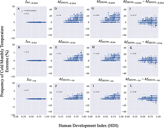
In addition to local monthly heat extreme frequency and HDI, we also investigated the relationship between frequency of local monthly cold extremes and HDI. Figure 7 shows the ensemble median change in frequency of local monthly cold temperature extreme exceedance plotted against HDI for land-based grid cells for the 20 year ZEC time frames. Like figure 6, changes in cold temperature extreme frequency were computed as the difference between ZEC90 and ZEC25 frequency distributions, and Spearman rank correlations were computed for each distribution.
Figure 7. Ensemble median monthly cold temperature extreme frequency in 20 year net zero baseline climatology (A)–(C) plotted against Human Development Index (HDI). Change in ensemble median monthly cold temperature extreme frequency in ZEC25 (D)–(F) and ZEC90 (G)–(I) windows plotted against Human Development Index. Marker sizes are based on population size, with a reference marker of 4 million people in panel (A). Panels (J)–(L) show the change in local monthly cold temperature extreme frequency evaluated as the ZEC90 frequency distribution (G)–(I) subtracted by the ZEC25 (D)–(F).
Download figure:
Standard image High-resolution image
During the net zero baseline climatology, land-based cold extreme frequencies are negligible based on ensemble median and are supported by results in figures 4(A)–(C). During the ZEC25 time frame, increased frequencies in cold extremes are evident across extreme thresholds following CO2 emissions cessation (figures 7(D)–(F)). Additionally, positive changes in Spearman rank correlations are calculated during the ZEC25 time frame due to the emergence in cold extreme frequency over high-HDI Northern Hemisphere land masses as shown in figures 5(D)–(F). The consistently positive Spearman correlations indicate that local cold monthly temperature extremes tend to impact higher HDI regions following CO2 emissions cessation, which is opposite to heat extreme trends where lower HDI regions continue to experience higher frequency of local monthly heat extremes for  and
and  thresholds. Over the remainder of the century after the ZEC25 time frame, Spearman rank correlations slightly increase which suggests that high HDI land regions will continue to experience higher frequency cold extremes after CO2 emissions cessation. In terms of ensemble median frequencies of cold extremes, nearly every populated grid cell experiences either no change or an increase in cold extreme frequency similar to the large-scale land-based cooling shown in the mean state regional climate projections post net zero (figure 3).
4. Conclusion
The ESMs included in the ZECMIP 1000 PgC ensemble project large-scale land based cooling during the 100 years following emissions cessation. However, there are significant differences in the value of ZEC regionally, consistent with recently published research (MacDougall et al 2022). Land regions are projected to experience a notably cooler local climate compared to the local climate in the 20 year baseline climatology (i.e. the climatology evaluated at the time of branching or emissions cessation). Though most land regions show a consistent cooling response after emissions cessation, there is evidence of continued increase of sea surface temperatures most obvious in the Southern and Indian oceans roughly between longitudes 70° W (Cape Horn, Chile) and 175° E (New Zealand).
Frequencies of local monthly hot temperature extremes are projected to remain either unchanged or decrease following CO2 emissions cessation. Land-based hot temperature extreme frequencies are projected to decrease as much as 40% within the century after net zero CO2 emissions, with largest reductions over land in the Northern Hemisphere. Reduction in land-based local monthly temperature extreme frequency within only a century after CO2 emissions cessation is a promising result, as heat extremes can have severe infrastructural impacts and can lead to loss of life. Within the ZEC25 and ZEC90 time frames, there are large areas with significant model agreement showing decreasing frequency of local monthly hot temperature extremes, however there are virtually no areas where models show significant agreement of how frequency of high temperature extremes are projected to change over the remainder of the century after ZEC25 time frame.
Although frequencies of land-based local monthly heat extremes are projected to remain constant or decrease, results show increasing frequency of extreme exceedance as high as +20% for 1 −3
−3 levels in the North Atlantic, North Pacific, Equatorial Pacific, and the Southern Ocean (especially south of Australia). This contrast between land-based and ocean-based extreme evolution could be an important consideration for planning purposes, as heat extremes can have devastating impacts on marine ecosystems (Garrabou et al
2009, Babcock et al
2019, Smale et al
2019, Holbrook et al
2020).
levels in the North Atlantic, North Pacific, Equatorial Pacific, and the Southern Ocean (especially south of Australia). This contrast between land-based and ocean-based extreme evolution could be an important consideration for planning purposes, as heat extremes can have devastating impacts on marine ecosystems (Garrabou et al
2009, Babcock et al
2019, Smale et al
2019, Holbrook et al
2020).
There is evidence of emerging land-based local monthly cold temperature extremes stemming from the rapid cooling over land following emissions cessation, with large scale mid- and high-latitude land regions having the highest increase in frequencies of cold monthly extremes after CO2 emissions cessation. There is strong model agreement to suggest that the emergence of local monthly cold extremes may be a concern following carbon dioxide emissions cessation, especially for mid- and high-latitude land regions with an emphasis on the Northern Hemisphere. However, like high temperature extremes, there are virtually no areas where changes in frequency of local monthly cold extremes over the century after the ZEC25 time frame show significant model agreement.
Over the century after CO2 emissions cessation, most land areas exhibit a decrease in temperature compared to the ocean due to the relative heat capacities of land and ocean. Decreases in regional temperature after net zero CO2 are larger over land in mid- and high-latitude Northern Hemisphere compared to tropical and equatorial latitudes. Changes in frequency of local monthly hot temperature extremes follow a similar pattern to regional temperature projections, where tropical and equatorial regions are projected to experience less decrease in local frequency of heat extremes than the decreases projected for mid- to high-latitude Northern Hemisphere. Since tropical and equatorial regions tend to have lower HDI than mid- to high-latitude Northern Hemisphere regions, the results suggest a continued or slightly enhanced disproportionality of climate change impacts on multi-decadal timescales even after net zero CO2 emissions are reached.
There is also a relationship between local HDI and changes in monthly cold extreme frequency but it follows the opposite sign as HDI and local monthly heat extremes; increases in the frequency of local monthly cold extremes are largest over the high-HDI Northern Hemisphere where the most significant mean state cooling is projected post-net zero CO2 emissions. This relationship suggests that cold extremes might impact higher HDI regions, especially mid- and high-latitude Northern Hemisphere, post CO2 emissions cessation.
This research has focused on idealized simulations of a net zero emissions where models are forced using the 1pctCO2 scenario, which lacks forcing from other greenhouse gases or aerosols, meaning the projections will not represent realistic future trajectories of net radiative forcing at a regional or global scale. In future studies, including other greenhouse gases and aerosols in the experimental setup would be valuable, as scenarios that included short-lived aerosols would likely lead to peak warming within the decade following emissions cessation (Dvorak et al 2022). Further investigation of commitments after emissions cessation at multiple cumulative emissions levels is also necessary as climate commitments are expected to change based on cumulative emissions levels at the time of emissions cessation (Ehlert and Zickfeld 2017). The A1 type of experiment used in this study assumes an abrupt transition to zero CO2 emissions which may introduce an unrealistic jolt to the climate system; future experimental designs might consider smoother transitions to net zero to avoid potential artificial shocks to the climate system in the model projections. In addition, since the ZECMIP ensemble only includes a small sample of models (n = 9), additional models would be beneficial for understanding significance and uncertainties and additional members of each model run would help differentiate model results from model internal variability.
Acknowledgments
This work was supported by the Australian Government National Environmental Science Program. The work was also completed with the assistance of resources from the National Computational Infrastructure (NCI), which is supported by the Australian Government.
Data availability statement
No new data were created or analysed in this study.
Supplementary data (12.1 MB DOCX)