

Abstract
This study investigates the epistemic uncertainty associated with the wave propagation modeling in wave climate projections. A single-forcing, single-scenario, seven-member global wave climate projection ensemble is used, developed using three wave models with a consistent numerical domain. The uncertainty is assessed through projected changes in wave height, wave period, and wave direction. The relative importance of the wave model used and its internal parameterization are examined. The former is the dominant source of uncertainty in approximately two-thirds of the global ocean. The study reveals divergences in projected changes from runs of different models and runs of the same model with different parameterizations over 75% of the ensemble mean change in several ocean regions. Projected changes in the wave period shows the most significant uncertainties, particularly in the Pacific Ocean basin, while the wave height shows the least. Over 30% of global coastlines exhibit significant uncertainties in at least two out of the three wave climate variables analyzed. The coasts of western North America, the Maritime Continent and the Arabian Sea show the most significant wave modeling uncertainties.
Export citation and abstract BibTeX RIS

Original content from this work may be used under the terms of the Creative Commons Attribution 4.0 license. Any further distribution of this work must maintain attribution to the author(s) and the title of the work, journal citation and DOI.
1. Introduction
Ocean wind waves play a key role in the impact the ocean may have on human activities. Wind waves transport more than half of the energy propagating across the ocean surface [1, 2], thus conditioning the shape and size of the elements confronting them, both in the open ocean (e.g. offshore structures [3] or vessels [4]) and in the coastal zone (e.g. coastal protection infrastructures [4, 5]). In line with the latter, the energy transported by waves shapes the coastline, eroding and moving materials, seeking to reach a natural equilibrium [6]. Extreme events of wind waves may therefore significantly impact offshore activities such as route shipping or the offshore wind industry [7, 8], and the coast, through flooding episodes [9, 10] and major erosion events [11, 12]. An accurate characterization of the wave climate and its variability is crucial for a range of applications, including infrastructure design and assessment of coastal impacts, among others.
Ocean wind waves are projected to change over the twenty-first century under a warming climate [13]. Climate change is affecting the main forcing of wind waves, the surface wind [14, 15], changing the transmitted energy [16] and, hence, the characteristics of the waves. In addition, the ice melting acceleration in high latitudes triggered by the increasing temperatures [17] is generating an expansion of wave generation areas [18, 19], thus inducing an increase in the wave energy propagating from the poles [20].
The assessment of the future behavior of wind waves under climate change has been a compelling subject of analysis for the last two decades [20–30], encouraged by the severe implications these changes may have, especially for extreme events [31, 32]. The standard approach to conduct these studies is based on wave climate projections [24–26, 33]. These products represent future wave climates, for different scenarios, developed using forcing drivers from global climate models (GCMs) or regional climate models (RCMs). Multiple studies on the matter have led to a community consensus about the projected behavior of climatological mean wave conditions in several ocean regions, such as an increase in significant wave height (Hs) in the Southern Ocean and in the tropical Eastern Pacific, and a decrease in the North Atlantic Ocean, Northwestern Pacific and Mediterranean Sea [21, 34]. The projected changes in extremes are, however, still characterized by great uncertainty [30, 35, 36].
The uncertainty associated with the projected changes in wind waves based on wave climate projection ensembles is normally assessed through the agreement in the sign and magnitude of the changes projected for the different ensemble members [24, 37]. Nevertheless, this integrated assessment is unable to unravel the origin of the uncertainties found. Several sources of uncertainty are present in assessing projected changes in wave climate conditions. Uncertainty propagates through all the stages involved in this assessment (figure 1), a process known as the uncertainty cascade [38, 39]. Lower steps within the uncertainty cascade will therefore accumulate the uncertainty inherited from top sources [40, 41].
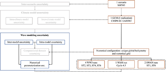
Figure 1. General outline of the uncertainty cascade related to the assessment of wave modeling uncertainty in wave climate projected changes. The left diagram depicts the uncertainty cascade. Colored boxes represent the sources of uncertainty linked to the projected changes assessed in this study. Right diagram displays the configuration of the experiment in relation to the sources of uncertainty.
Download figure:
Standard image High-resolution imageBeyond the aleatoric uncertainty associated with the chaotic natural variability of the climate variables involved [38, 39], the uncertainty in wave climate projected changes also integrates the socio-economic scenario uncertainty, the uncertainty related to GCMs and the epistemic uncertainty associated with the wave modeling part. These sources of uncertainty are usually embraced by including representative members of different configurations. For example, it is common practice to include several scenarios and GCM forcings to consider these uncertainties in the assessment [30, 42]. The use of different wave models and/or wave model setups, however, is uncommon in studies of this kind.
This study particularly focuses on the epistemic uncertainty associated with the wave modeling component of the simulations in wave climate projections. Wave models (e.g. SWAN, WAM) reproduce the generation, propagation and dissipation of wind waves through numerical equations, but have inherent simplifications that cause the numerical output to diverge from reality. Model differences mainly arise from the numerical scheme used to solve the governing equations, the number of wave propagation features modeled (e.g. bottom friction, white-capping, ice interaction) and the equations used to represent each of these features. Model internal parameterization can also be tuned, leading to variations between runs of the same model [43]. In this context, predefined internal parameterizations, known as source term packages, are available. These source terms packages comprise a set of equations that address the wave generation and dissipation, also including some tunable parameters. Nevertheless, these source terms packages do not encompass the entire model parameterization, as some other issues, such as the wave–bottom interaction, fall outside of them and can also affect the wave model outcomes.
To date, only a very few studies have addressed the uncertainty associated with wave modeling in projected changes in wave climate [21, 22]. These studies assessed the contribution of wave modeling uncertainty to the total uncertainty in the projected changes, distinguishing its significance from other sources such as those associated with the GCMs and the future scenarios. Nevertheless, a specific study that focuses on isolating and analyzing in detail the epistemic uncertainty related to wave modeling has not yet been conducted. Thus, several questions still arise and remain unanswered, such as the actual influence of wave model selection on projected changes in wave climate, the extent to which the parameterization of the numerical model affects the changes, and which of these sources of uncertainty is more significant. The aim of this study is to address these and related questions by isolating the epistemic uncertainty associated with wave modeling, examining the relative importance of its main sources in wave climate projected changes, and quantifying its magnitude.
2. Methods
2.1. Wave climate projection ensemble
This study uses a wave climate projection ensemble forced by a single run (r1i1p1f1) of the CMIP6 [44] GCM EC-EARTH3 [45], which has been proven to perform well in reproducing climate metrics [46], and a single future climate scenario (SSP5-8.5 [47, 48]). Runs use three-hourly surface wind fields and daily ice coverage fields as forcings (more details in previous articles [43, 49]). The time slices 1995–2014 and 2081–2100 are used as baseline and future periods, respectively. The wave climate projection ensemble is produced using the most popular wave models within the climate community: WaveWatch III v6.07 [50] (hereinafter WW3), WAM v4.6 [51] and SWAN v41.20AB [52, 53].
The three models used are third-generation spectral wave models that share a similar theoretical background. The main characteristic of this type of models is not restricting the shape of the wave spectrum as in previous generations. All of them are based on the solution of the action balance equation (equation (1))
where  is the wave action density, c is the propagation celerity of the wave energy,
  is the intrinsic frequency and
  is the propagation direction.
  is the total sum of source terms of different physical processes parameterized in the model.
WAM and WW3 use explicit numerical propagation schemes limited by time steps due to Courant–Friedrichs–Lewy (CFL) criteria, whereas SWAN uses an iterative approximation to a fully implicit scheme to avoid such limitations [54, 55]. As a result, WW3 and WAM models are more efficient in regional and global domains, whereas SWAN model is computationally more efficient in coastal areas. Models are also different regarding the processes solved and the parameterizations used to solve them. SWAN model differs from WAM and WW3 on including coastal-specific parametrizations (e.g. triads, quadruplets) to solve processes in limited water depths and complex coastal areas. All this makes WAM and WW3 models to be typically used for global [56–61] and regional [42, 62–64] scales, while SWAN model is extensively used to develop coastal-scale studies [65–67].
Each ensemble member is developed using a wave model with a different numerical parameterization. Differences lie in the source term package selected to develop each ensemble member. Default parameters are employed for each simulation. The ensemble comprises seven members, integrating four WW3 runs developed with the source term packages ST2, ST3, ST4 and ST6, two SWAN runs with the source term packages ST1 and ST6 and one WAM run with the Cycle 4.5 source term package. Each source term package parameterization implements different approximations for the wind–wave interaction and the wave dissipation. A succinct definition of each source term package is provided in supplementary material.
Each ensemble member produces a global three-hourly time series of significant wave height (Hs), mean wave period (Tm) and mean wave direction (θm), with one-degree spatial resolution. Grid nodes covered by ice for more than 30% of time are not considered in the analysis. A global validation against buoy and reanalysis data has been undertaken [49]. A detailed description of the numerical configuration of the experiments can be found in two previous articles [43, 49].
2.2. Projected changes in wave climate
Projected changes are computed as the relative projected change (in %) between the baseline period and the future period, normalized by the historical value. In the case of wave direction, the relative projected changes are normalized by 360°.
2.3. Analysis of variance
The relative contribution to the total uncertainty between the wave model used and the model parameterization—i.e. the inter-model and intra-model uncertainties, respectively, is estimated through a one-way analysis of variance (one-way ANOVA), similarly as it has been done in previous studies [22, 40]. ANOVA method is used to compute the explained variance ( ; equations (2) and (3)) of each source of uncertainty based on the sum of squares (
 ) between individual member runs [68, 69].

where  is the total SS and
  is the SS between wave models:
where  is the relative projected change for run
  of model
  ,
,  is the mean relative projected change of model
  runs,
runs,  is the overall mean projected change and
  is the number of runs of each propagation model.
2.4. Quantification of uncertainty
The inter-model and intra-model uncertainties are independently quantified by assessing the differences between the projected changes from different wave models and different model parameterizations, respectively. Discrepancies are measured through the relative mean difference (RMD) metric, computed as:
where  and
and  represent the relative change in runs
  and
and  , respectively; and
  represent the ensemble mean relative change.
The inter-model uncertainty ( ; equation (4)) is quantified by computing, first, the RMDs between runs from each possible combination of wave models (i.e. WW3–SWAN, WW3–WAM and WAM–SWAN). Thus, the number of RMDs between two different wave models is equal to the number of runs for the first model multiplied by the number of runs for the second one. Since the number of runs differs between models, so does the number of RMDs for each model combination. Thus, a weighted mean and a weighted standard deviation are computed, to avoid results biasing, as follows:

where,  is the weighted mean uncertainty and
  is the weighted standard deviation of the uncertainty, estimated as:
where N is the number of combinations,  is the mean RMD for the combination
  and
and  is the number of elements within combination
  .
.
The intra-model uncertainty ( ) quantification is analogous to the inter-model uncertainty (equation (4)). RMDs are computed between model runs from the same wave model with a different numerical parameterization. However, since the different number of model runs would lead to a strong imbalance between the number of RMDs for each wave model (six for WW3, one for SWAN, none for WAM), only the runs for WW3 are considered to quantify
  .
.
2.5. Significance of uncertainty
The relevance of uncertainty is assessed to identify areas where it may have a greater impact. This is achieved by evaluating the magnitude of uncertainty, the projected changes, and the discrepancies among members. Thus, a specific ocean location (i.e. ocean grid point) is considered to have significant uncertainty if the mean uncertainty value is greater than 25% (the same approach is applied for inter- and intra-model uncertainties). In addition, uncertainty values are deemed significant if the absolute ensemble mean projected changes exceed the absolute global median projected change and/or if the standard deviation of individual member projected changes is greater than twice the ensemble mean projected change. The latter two conditions aim to exclude regions exhibiting very high uncertainty values, which arise from low ensemble mean values derived from low individual member changes.
3. Results
This study isolates and quantifies the wave modeling epistemic uncertainty. To that end, a single-scenario, single-forcing wave climate projection ensemble developed with multiple wave models and parameterizations is used (see section 2). Using a single scenario and a single forcing GCM avoids attributing inter-member divergences to the uncertainty associated with the scenario and the forcing climate model. In the same vein, all numerical propagation runs are developed, as much as possible, using the same bathymetry and computational grid [49], hence avoiding model set-up discrepancies. The differences can, therefore, only be attributed to the numerical parameterization of the model—in other words, to the wave modeling epistemic uncertainty. This is illustrated in figure 1. The colored boxes in the uncertainty cascade depict the sources of uncertainty associated with the projected changes assessed in this study. In contrast, the gray boxes represent sources of uncertainty not linked to the discrepancies observed among ensemble members.
The wave modeling epistemic uncertainty can be seen as the addition of two sources of uncertainty: (i) the selection of the numerical model and (ii) the internal parameterization of the model. Regarding the former, each numerical model has some specific features not shared with the others, thus inducing differences in the results. On the other hand, despite all model runs sharing most of the numerical parameterization, the numerical approximation of some specific processes may differ. This study considers both sources of uncertainty by including numerical simulations developed with different wave models and with different parameterizations of the same model (see section 2).
The discrepancies between ensemble members are addressed in figure 2. Figure 2 shows the regional and global (ocean regions are defined in figure SM1) uncertainty cascades [40] for projected changes (see section 2) in mean Hs, Tm and θm (panels (a)–(c), respectively). Each cascade is divided in three levels. From top to bottom, each level displays the ensemble mean projected change, the wave model mean projected changes, calculated as the mean change from all members of a specific model, and the projected change for each ensemble member, along with the 5%–95% range (assuming normal distribution). Results for 99% percentile Hs (Hs99) are also assessed and shown in figure SM2. The width of the displayed uncertainty cascades reflects the divergence between ensemble members (lower level) and wave models (intermediate level). Projected changes in mean Hs (figure 2(a)) show the greatest differences in the North Pacific Ocean. In particular, TWNP is the ocean region where the greatest differences between member runs (from −9.5% to −5%) and wave model means (from −8.5% to −4.8%) can be seen. On the other hand, TESP shows the lowest differences. Note that most regions show an agreement between all ensemble members in terms of the sign of change. The main exceptions are TESP, ETSA and ETSI, where two out of the seven members diverge in this change feature. Projected changes in Hs99 (figure SM2) show the greatest differences in TWNP and TWSP. Additionally, only TNIO shows discrepancies in the sign of change between ensemble members.
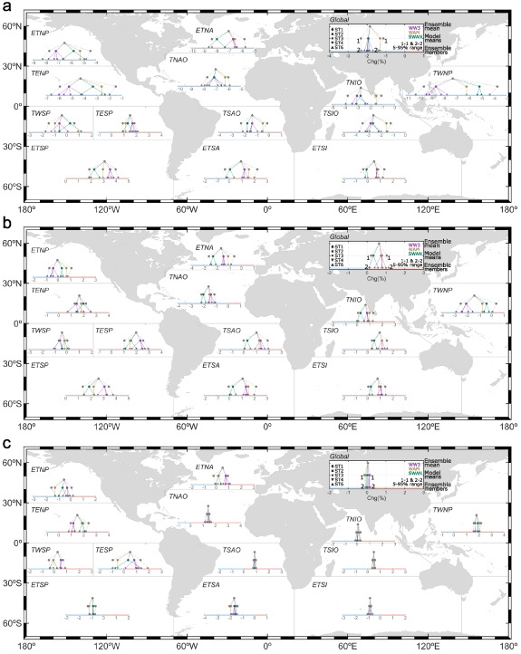
Figure 2. Uncertainty cascades for (a) mean Hs, (b) mean Tm and (c) mean θm. Projected changes, per region and globally. Lower levels of the cascades represent more disaggregated changes: Top level—ensemble mean relative change, intermediate level—wave model mean relative changes, and lower level—ensemble member relative changes. Outside gray dashed lines represent the 5%–95% range. WAM—Cycle 4.5 is displayed as ST4 for the sake of simplicity.
Download figure:
Standard image High-resolution imageProjected changes in Tm (figure 2(b)) show a general homogenous behavior between ocean regions as most of them show 5%–95% ranges for individual member runs lower than 2.5%. TWNP is the only exception, showing a 5%–95% range between ensemble members of approximately 3%. Changes in mean θm (figure 2(c)) show the strongest spatial heterogeneity across ocean regions among all the wave climate metrics analyzed. In general, except for ETNA, the differences are significantly higher in the Pacific Ocean than in the rest of the ocean basins, especially in the tropical region. On the other hand, regions such as TNAO, TSAO and TSIO show very good agreements between individual member runs and wave models, with differences lower than 1% in both cases. For completeness, the individual member projected changes and the ensemble mean changes across the global ocean are included in figures SM3–6.
The relative importance between the wave model used and its internal parameterization within the total wave modeling uncertainty in wave climate projected changes (i.e. inter-model and intra-model uncertainty, respectively) is assessed through an ANOVA (see section 2). Figure 3 presents the results, illustrating that, for example, the uncertainty in global projected changes in mean Hs is approximately 80% attributable to the chosen model and 20% to the model setup configuration. Results show an overall higher contribution of the inter-model uncertainty to the total uncertainty with respect to the intra-model uncertainty—namely, the use of different models has a greater influence on the differences found in the wave climate projected changes than the use of different model parameterizations. In fact, at least 60% of the ocean regions show a higher importance of the inter-model uncertainty for each metric analyzed (69%, 62%, 85% and 62% for mean Hs, Hs99, mean Tm and mean θm, respectively).
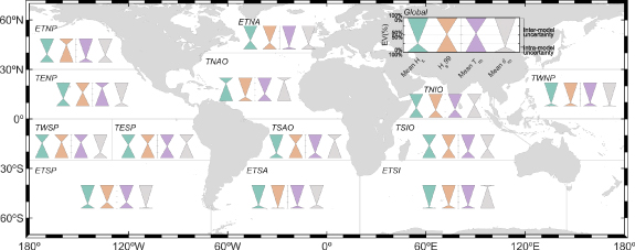
Figure 3. Relative contribution to the total wave modeling epistemic uncertainty, expressed as the explained variance (in %), for projected changes in mean Hs, Hs99, mean Tm and mean θm, per region and globally, between the inter-model (EVinter, equation (1)) and intra-model (EVintra, equation (2)) uncertainties.
Download figure:
Standard image High-resolution imageAcross extra-tropical regions, the inter-model uncertainty for mean Hs remains above 60% relative to intra-model uncertainty, regardless of the region analyzed. In tropical regions this pattern is not so clear, as there are regions where the contribution of the model parameterization to the total uncertainty is considerably higher than the wave model used (e.g. TNAO, TWSP). Other regions such as TSIO, TNIO and TESP show a split dominance between both sources of uncertainty. The behavior of Hs99 is, in general terms, very similar to the one for mean Hs. Main exceptions can be found in ETNP and TNAO, where the intra-model uncertainty clearly dominates over the inter-model uncertainty for Hs99 and the opposite for mean Hs. The analysis of the projected changes in mean Tm evidence that this parameter is the one in which the selection of the wave model plays a more important role in contrast to the model parameterization in the total uncertainty found, as more than 75% of the regions show this behavior. Only TENP and TWSP show opposite results, both with a relative importance of the intra-model uncertainty above 65%. The analysis of mean θm shows a great heterogeneity in the Southern Ocean as the main outcome. In this regard, while ETSP and ETSA show the relative importance of the inter-model uncertainty higher than 80%, ETSI shows the opposite behavior with less than 10%.
Nevertheless, results from figure 3 only informs about the relative importance of each contributing element and nothing about the total amount of uncertainty of each source. In order to compare the existing uncertainty between regions, a regional (and global) quantification of both sources of uncertainty (see section 2) for mean Hs, Hs99, mean Tm and mean θm is provided in figure 4. For each metric, the mean inter-model and intra-model uncertainties, along with the confidence intervals (estimated as the mean ± one standard deviation) are displayed.

Figure 4. Quantification of the inter-model and intra-model wave modeling epistemic uncertainty for projected changes in mean Hs, Hs99, mean Tm and mean θm, per region and globally. Black arrows indicate values higher than 100%.
Download figure:
Standard image High-resolution imageThe highest uncertainties in mean Hs are found in TWSP, exceeding mean values of 100% for both inter- and intra-model uncertainties. The former also shows mean values over 100% in ETSA and ETSI. Note that figure 2 shows great discrepancies between SWAN and the other two wave models in the latter two regions, likely causing the high inter-model uncertainty values found. On the other hand, it is also worth noticing the low uncertainties found for projected changes in mean Hs in the Northern Hemisphere, especially in the Atlantic Ocean, where the inter- and intra-model uncertainties show mean values lower than 15%. Hs99 shows the greatest uncertainties in the tropical latitudes of the Indian Ocean, exceeding mean values of 70% for both the inter- and intra-model uncertainties, likely due to the higher differences between WAM and the rest of the wave models in these regions (figure 2).
The inter-model uncertainty for mean Tm exceeds mean values of 50% in 7 out of the 13 regions analyzed. This denotes Tm to be the parameter for which the selection of the wave model causes the greatest differences in the estimated projected changes. On the other hand, only two regions (ETNP and TWSP) show mean values of intra-model uncertainty above 60%. Regarding mean θm, as expected from the results presented in figure 2, sensitive differences can be seen between regions. Inter-model uncertainties in ETNP, TWSP, TESP, ETNA and TNIO exceed mean values of 90%, whereas for the rest of the regions, it shows mean values always lower than 40%. The same conclusions can be extracted for the intra-model uncertainty: while ETNP, TESP and TNIO show mean values above 60%, the rest of the regions show values lower than 30%.
Despite figure 4 allowing the identification of the regions showing the highest wave modeling uncertainties, it precludes identifying precisely in which areas these uncertainties are more important. The fact that RMDs are computed by normalizing with the ensemble mean (see section 2), leads to large uncertainties where the ensemble mean changes are very low. Thus, it is relevant to distinguish between cases in which low ensemble mean changes are caused by low individual member changes, from ocean areas where ensemble mean changes are very low due to the balance between strong individual change signals of different signs. Figure 5 depicts the ocean areas where the inter- and intra-model uncertainties are significant for the projected changes in mean Hs, Tm and θm (see section 2). It identifies ocean areas where the high uncertainties found are relevant due to the magnitude of the projected changes and/or due to the great discrepancies between members. Correspondingly, it facilitates the identification of ocean regions where the wave modeling uncertainty is not critical in the assessment of wave climate projected changes. Results for Hs99 are included in figure SM7.

Figure 5. Ocean areas showing significant (a) inter-model and (b) intra-model wave modeling uncertainty for mean Hs (blue), mean Tm (green) and mean θm (orange) projected changes. Stippling indicates significant uncertainties for the three metrics analyzed.
Download figure:
Standard image High-resolution imageResults indicate that inter-model uncertainty is more important than intra-model uncertainty across the global ocean. In this regard, the proportion of the global ocean showing a significant inter-model uncertainty for mean Hs, Tm and θm is always higher than 25%, whereas for the intra-model uncertainty the percentages are always lower than 25%. Figure 5(a) shows that the ocean areas where the inter-model uncertainty is significant simultaneously for the three metrics analyzed (8% of the ocean surface) are mainly in the Pacific Ocean, particularly at TENP. Other small ocean areas in the Atlantic Ocean (e.g. tropical northeast) and Indian Ocean (e.g. western Arabian Sea) also show this behavior.
The inter-model uncertainty in projected changes in mean Hs is notably important in the tropical Pacific basin and the Gulf of Alaska. Some dispersed areas in the Atlantic and Indian Oceans also show significant results, such as the southernmost part of the Atlantic, the seas south of Sumatra and Java and the Arabian Sea. Mean Tm presents the largest proportion of the global ocean showing significant inter-model uncertainties (53%). Most of the Pacific basin, with the only exception of the western extra-tropical region, shows this behavior. Additionally, a great proportion of the Northwest Atlantic Ocean and the tropical north Indian Ocean also show significant inter-model uncertainties for this metric. Regarding the projected changes in mean θm, the Pacific Ocean is again the basin where this source of uncertainty is more relevant, especially in the tropical and the western extra-tropical ocean regions. The tropical North Atlantic and the Arabian Sea also show significant inter-model uncertainties.
The proportion of the global ocean showing significant intra-model uncertainties for all the metrics analyzed is very low (<1%; figure 5(b)). Besides, among the three metrics, mean Hs shows significant results in the smallest proportion of the ocean (8% vs. 23% and 20% for mean Tm and θm, respectively). Ocean areas showing significant intra-model uncertainty for mean Hs projected changes are mainly located in tropical latitudes, in both the Pacific and Indian Oceans. Regarding the projected changes in mean Tm, ocean areas showing significant intra-model uncertainties are sparsely distributed across all ocean basins. Among them, the easternmost part of the Pacific Ocean shows the clearest results. Finally, projected changes in mean θm show the most significant results in the extra-tropical and eastern tropical regions of the Pacific Ocean.
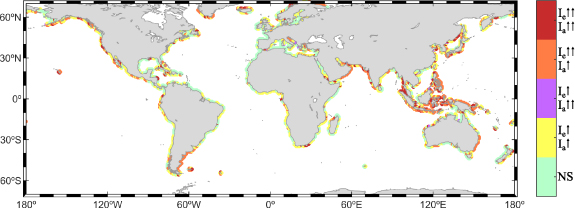
Significant uncertainties may have severe implications where the wave climate is a key process driver, as in the coastal zone, where waves play a key role in coastal processes such as flooding or erosion [31, 70]. Figure 6 depicts qualitatively the degree of wave modeling uncertainty along the global coastlines. To that end, the number of wave climate variables in which the uncertainty is found to be significant is computed for both inter-model and intra-model uncertainties. Three variables have been deemed in accordance with the analysis presented in figure 4: wave height (through mean Hs), wave period (through mean Tm) and wave direction (through mean θm). Results indicate that more than 35% of the global coastlines show significant uncertainties in at least two out of the three metrics analyzed for the inter-model and/or intra-model uncertainties (orange, purple and red in figure 6). On the other hand, 27% of the global coastlines does not show significant wave modeling uncertainties (green in figure 6). The coasts of Oman, Iran, Pakistan and India, the coasts of the Maritime Continent, the western coasts of North America and the eastern coasts of Russia and Japan show the most significant wave modeling epistemic uncertainty.
Figure 6. Integrated qualitative assessment of the inter-model and intra-model uncertainty significance for the assessment of projected changes in wave climate along the global coastlines. Two upward arrows indicate that at least two out of the three wave climate metrics analyzed show significant uncertainty in projected changes. One upward arrow indicates that one or less of the three wave climate metrics analyzed show significant uncertainty in projected changes. The green color highlights the case where both sources of uncertainty show no significance (NS) in wave climate projected changes. The wave climate metrics analyzed are mean Hs, mean Tm and mean θm.
Download figure:
Standard image High-resolution image
4. Conclusions and discussion
Over the past two decades, significant progress has been made in examining the effect of climate change on wind waves, largely due to the concerted efforts of the Coordinated Ocean Wave Climate Project (COWCLIP) [23, 71, 72]. Despite its inevitable role as a primary source of uncertainty in such studies, the epistemic uncertainty associated with wave modeling has been addressed in only a limited number of researches [21, 22]. This study has specifically analyzed this source of uncertainty in wave climate projected changes (figure 1) by isolating it from other sources also present in assessments of this kind (e.g. GCM-related uncertainty, scenario-related uncertainty). The analysis has been conducted based on a seven-member, single-scenario, single-forcing wave climate projection ensemble. Three numerical wave models have been selected to develop the ensemble members (WW3, WAM and SWAN). Two primary sources of uncertainty within the wave modeling uncertainty have been independently analyzed: the inter-model uncertainty, which considers the differences between models; and the intra-model uncertainty, which considers the differences between model parameterizations. Furthermore, all members share a consistent numerical domain with the ultimate objective of reducing to the minimum the differences between members attributable to this factor. Although the findings presented in this research are intrinsically influenced by the number of members utilized and their distribution between propagation models, the ensemble framework encompasses a substantial number of members, developed with the most prevalent wave models in wave climate projections and their most common parameterizations. Collectively, this offers comprehensive coverage of the most probable scenarios encountered in investigations of this nature.
Results have demonstrated that both the selection of the wave model and the internal parameterization of the model affect the value of the estimated wave climate projected changes. In general, the differences between wave models exhibit higher uncertainty with respect to the internal parameterization of the model. In fact, over 60% of the ocean regions analyzed (figure 3) have shown a larger contribution from inter-model uncertainty compared to intra-model uncertainty for all metrics analyzed, although the latter is always present too. This conclusion is even more robust when considering that the intra-model uncertainty is estimated from four WW3 models runs, of which two are outdated (i.e. ST2 and ST3) with respect to the remaining two (i.e. ST4 and ST6). However, while the dominance of the inter-model uncertainty with respect to the intra-model uncertainty is clear in the extra-tropical region, it is not as clear in tropical latitudes. Uncertainty has also been quantified by assessing the divergences between members (figure 4). The inter-model uncertainty has shown mean values exceeding 50% in 31%, 23%, 54% and 38% of the ocean regions for mean Hs, Hs99, mean Tm and mean θm, respectively. In contrast, values for intra-model uncertainties are 8%, 23%, 15% and 23%. It is important to note that, on average, for both cases, the projected changes in mean Tm exhibit the greatest uncertainty, particularly in the Pacific Ocean.
A more detailed analysis has determined in which ocean areas the wave modeling epistemic uncertainty is significant (figure 5). To that end, the uncertainty values have been analyzed together with the magnitude of the projected changes and the deviations between members. The period of the waves has been found to be the wave climate variable showing the greatest uncertainties across the ocean (53% and 23% of the ocean surface for inter- and intra-model uncertainties, respectively). After the wave period, the direction is the wave characteristic showing significant uncertainties in a larger ocean area (42% and 20%) and, finally, the wave height, which shows the lowest proportion (29% and 8%). Particularly, the Pacific Ocean stands out as the basin where significant uncertainties have been found in larger areas. On the contrary, the Tropical South Indian Ocean and extra-tropical southern regions of the Atlantic and Indian Oceans exhibit the least significant uncertainties. Additionally, figure 6 shows that a high proportion of the global coastlines is affected by significant wave modeling uncertainties. In fact, 80% of them show significant inter-model and/or intra-model uncertainties in at least one out of the three wave climate variables analyzed, and over 30% in at least two of them. Thus, using one model or another leads to results with differences that cannot be neglected for processes where these variables are involved.
This study has demonstrated that the assessment of projected changes in wave climate based on a single wave model with a unique configuration—which is also the most common approach—may be affected by relevant wave modeling uncertainties, and eventually bias the results. These uncertainties cascade and become critical to study changes in processes that use the wave climate as a driver, such as coastal erosion [32, 73] and flooding [31, 74, 75]. Using multiple models with different configurations may be a suitable approach to address the epistemic uncertainty in wave climate projection assessments. However, developing wave climate projection ensembles requires extensive computational time and resources, so including multiple wave models and/or parameterization may imply a considerable increase in the demands. Hence, until computational resources allow for such an approach, it is strongly recommended to perform extensive calibration and validation of the simulations to select the most appropriate model and parameterization, and minimize the discrepancies with the real ocean surface.
Results presented here serve as a basis to understand the scope of the wave modeling uncertainty in wave climate projections. They underscore the need for additional investigation into the origin of the observed uncertainties. The parameterization of processes such as the energy transfer from the wind to the ocean and the wave energy dissipation are examples of likely causes for the differences found among the projected changes of ensemble members. Specific studies that isolate these processes are required to elucidate the distinct contribution of such processes to wave modeling uncertainty. Such insights will ultimately help to provide a more rigorous description of the projected changes and their robustness.
Acknowledgments
The authors greatly appreciate the valuable comments from Mark Hemer and Jean Bidlot, which have helped to improve this manuscript. HL and MM acknowledge financial support by CoCliCo project, which received funding from the European Union's Horizon 2020 research and innovation program under Grant Agreement No. 101003598, and the ThinkInAzul programme, with funding from European Union NextGenerationEU/PRTR-C17.I1 and the Comunidad de Cantabria. GL acknowledges financial support of Portuguese Fundação para a Ciência e a Tecnologia I.P./MCTES through national funds (PIDDAC)—UIDB/50019/2020—Instituto Dom Luiz.
Data availability statement
The data that support the findings of this study are available upon reasonable request from the authors.
Supplementary data (3.9 MB PDF)