

Abstract
Deriving hyperlocal information about fine particulate matter (PM2.5) is critical for quantifying exposure disparities and managing air quality at neighborhood scales in cities. Delhi is one of the most polluted megacities in the world, where ground-based monitoring was limited before 2017. Here we estimate ambient PM2.5 exposure at 100 m × 100 m spatial resolution for the period 2002–2019 using the random forest model. The model-predicted daily and annual PM2.5 show a ten-fold cross-validation R2 of 0.91 and 0.95 and root mean square error of 19.3 and 9.7 μg m−3, respectively, against coincident ground measurements from the Central Pollution Control Board ground network. Annual mean PM2.5 exposure varied in the range of 90–160 μg m−3 in Delhi, with shifts in local hotspots and a reduction in spatial heterogeneity over the years. Mortality burden attributable to ambient PM2.5 in Delhi increased by 49.7% from 9188 (95% uncertainty interval, UI: 6241–12 161) in 2002 to 13 752 (10 065–19 899) in 2019, out of which only 16% contribution was due to the rise in PM2.5 exposure. The mortality burden in 2002 and 2019 are found to be higher by 10% and 3.1%, respectively, for exposure assessment at 100 m scale relative to the estimates with 1 km scale. The proportion of diseases in excess mortality attributable to ambient PM2.5 exposure remained similar over the years. Delhi can meet the United Nations Sustainable Development Goal 3.4 target of reducing the non-communicable disease burden attributable to PM2.5 by one-third in 2030 relative to 2015 by reducing ambient PM2.5 exposure below the World Health Organization's first interim target of 35 μg m−3. Our results demonstrate that machine learning can be a useful tool in exposure modelling and air quality management at a hyperlocal scale in cities.
Export citation and abstract BibTeX RIS

Original content from this work may be used under the terms of the Creative Commons Attribution 4.0 license. Any further distribution of this work must maintain attribution to the author(s) and the title of the work, journal citation and DOI.
1. Introduction
Exposure to ambient fine particulate matter (PM2.5) is the second-largest health risk in India (Balakrishnan et al 2019), resulting in 0.98 million (95% uncertainty interval, UI: 0.77–1.19) deaths in 2019 (a 115.3% increase from 1990) and 1.36% loss in the country's gross domestic product (Pandey et al 2021). Within India, the highest level of exposure was found in the megacity Delhi (Dey et al 2020). The problem of air pollution in the megacity Delhi was recognized a long time ago, and numerous efforts were undertaken to manage air quality with mixed results. The first step taken by the policymakers to manage air quality was commencing systematic air pollution monitoring decades ago. Measurements started first for total suspended PM2.5 and then for PM2.5 smaller than 10 μm by the Central Pollution Control Board (CPCB). Monitoring of PM2.5, the most important criteria pollutant from a health standpoint, started only after 2009–2010 in Delhi, and till 2017, the number of monitoring stations was limited to less than 10. The number of stations rapidly increased to 40 by 2022 (figure S1, supplementary information, SI) in response to widespread concern about air quality, more particularly the seasonal degradation during October–January, and its associated health impacts estimated by the Global Burden of Disease India study and various other studies in the last decade (Guttikunda and Goel 2013, Joshi et al 2021, Krishna et al 2021). More recently, efforts have been made to identify sources in real-time (Lalchandani et al 2021) in Delhi.
During the last decade, several policy interventions were taken by the Government of India (GoI) to manage air quality in Delhi. A graded response action plan (GRAP) was implemented (CPCB 2017), where specific control measures were adopted based on the air quality index values. An air quality forecasting system was developed for the Delhi national capital region (NCR) to facilitate GRAP implementation preparedness (Jena et al 2021). The national clean air program (NCAP) was launched in 2019 with a target of reducing the PM2.5 level to 132 non-attainment cities by 30% in 2024 relative to its 2017 level (https://prana.cpcb.gov.in/#/home). A separate Commission for Air Quality Management has been constituted for the independent supervision of the clean air action plan implementation in Delhi NCR. While all these efforts are no doubt made in the right direction, it is critical to have a long-term PM2.5 database with a high spatial resolution for evaluating the efficacy of air quality management plan. With the current PM2.5 monitoring network, Delhi has managed to meet at least one monitor per million population tar get (Martin et al 2019), but the data period is too short for any trend analysis. Moreover, the network is disproportionately distributed across the city (figure S1), leaving many municipal wards of the city unmonitored.
To address the paucity of ground-based PM2.5 in Delhi and, more generally, in India, Dey et al (2020) have developed a national ambient PM2.5 database at a spatial scale of 1 km × 1 km using satellite-derived aerosol optical depth (AOD) from 2000 onwards. This data has been recently used by many epidemiological studies to generate indigenous evidence of the health impacts of air pollution in India (Spears et al 2019, deSouza et al 2022). Another study (Mandal et al 2020) developed ambient PM2.5 exposure data, only for Delhi NCR, at the same 1 km scale using a machine learning technique for a limited period (2010–2016) and utilized it for health study (Prabhakaran et al 2020). Hyper-localized measurements of air pollution in Delhi (Kumar et al 2020) and other urban centers (Vu et al 2019), monitoring on a mobile platform (Apte et al 2011), and the data from the low-cost sensors (Hagan et al 2019) revealed that PM2.5 varies at sub-km scale.
There have been several attempts to derive PM2.5 information at a hyperlocal scale. (Di et al 2019) used a generalized additive model to combine PM2.5 estimates from the neural network, random forest, and gradient boosting on multiple predictor variables for the United States with ten-fold cross-validated R2 of 0.86 and 0.89 for daily and annual PM2.5. In another study, (Huang et al 2021) used a similar method to downscale PM2.5 prediction at 100 m resolution without degrading the model performance. However, no such study exists in the literature for India or other low- and middle-income countries. The 1 km national data (Dey et al 2020) is not spatially resolved enough to provide air quality information at a neighborhood scale within the non-attainment cities, which is required to track the local influences on air quality and the disparity in exposure across neighborhoods. Moreover, a high spatially resolved PM2.5 estimate is expected to improve exposure attribution.
Furthermore, the mortality burden attributable to ambient PM2.5 exposure has been rising in Delhi (Balakrishnan et al 2019). The rise in health burden is a cumulative effect of the year-to-year changes in exposure and baseline mortality of non-communicable diseases (NCDs) and an increase in population (Chowdhury et al 2020). For Delhi, the relative contributions of these factors in modulating the health burden are not known. Furthermore, the current temporal trend in health burden cannot be extrapolated to estimate the burden in the future since the trend of exposure may vary in view of policy interventions. One of the key targets of the United Nations (UN) sustainable development goal (SDG) 3.4 is to reduce the NCD burden by one-third in 2030 relative to the 2015 level. If the current trends in age-distributed population and baseline mortality continue, PM2.5 exposure needs to be reduced by a bigger margin to reduce the overall health burden. The present study addresses these critical knowledge gaps and is novel in three different ways.
First, we develop a machine learning-based model to map PM2.5 at an ultra-high (100 m × 100 m) resolution in the megacity Delhi for the period 2002–2019. This allows us to examine the spatiotemporal changes in ambient PM2.5 exposure at the municipal ward level for the first time. Secondly, we estimate the changes in associated health burden during this period and isolate the contributing factors. Finally, we set the exposure reduction target for Delhi to meet the UN SDG3.4 goal that requires efforts beyond the current NCAP.
2. Data and analysis
Delhi is inhabited by over 20 million population and caters to millions more daily who travel every day to the megacity for jobs. For the exposure assessment at a hyperlocal scale, we first build a machine-learning model using the predictor variables chosen based on the literature review (de Hoogh et al 2018, Vu et al 2019, Chen et al 2020). The methodology is explained below.
2.1. Random forest (RF) model
We choose the RF model as the machine learning tool to predict PM2.5. RF is a supervised machine learning model that works by averaging a set of decision trees that calculates the best predictions based on a subset of predictors (Breiman et al 2001). The RF model's advantages include its accuracy in learning and classifying features, its ability to include many input variables, and its output of variable importance. The model selects a random subset of samples from all observations with replacement and subsequently selects the best set of predictors that provides the best split at each node (Breiman et al 2001). We divide the data set into 70% and 30% for training and testing, respectively
The predictor variables used in the model training (summarized in table S1 in SI) are available at various spatial resolutions. AOD is one of the key predictor variables in our model. We process AOD data retrieved by the Moderate Resolution Imaging Spectroradiometer (MODIS) at 1 km × 1 km spatial resolution (Lyapustin et al 2018). MODIS AOD has been previously validated in India and used to generate the national PM2.5 database for India (Dey et al 2020). We consider meteorological data of nine variables (table S1) for the study period from the European Centre for Medium-Range Weather Forecasts data archive (Hersbach et al 2020). Elevation data from the Advanced Spaceborne Thermal Emission and Reflection Radiometer Global Digital Elevation Map is downloaded from EARTHDATA for Delhi, India, at a resolution of 30 m. For the population data, we use LandScanTM yearly population statistics for the period 2002–2019. Land use land cover parameters at 500 m resolution (open shrubland, bare/sparse vegetation, waterbodies, and artificial/urban areas) for the years 2002–2019 were derived from MCD12Q1 version 6. Normalized difference vegetation index (NDVI) data at 250 m spatial resolution (MOD13Q1 Version 6) is downloaded from the LAADS DAAC. Since NDVI is produced at 16 day intervals, every 15 days preceding the day with measured NDVI was given the same NDVI values. Road Network Data is downloaded as an ArcGIS-ready shapefile from the OpenStreetMap project through Geofabrik and processed in ArcGIS. The road network map is classified into three classes—motorways, primary and trunk roads, and secondary and tertiary roads. We estimate the distance (in meters) between the centroid of each 100 m × 100 m grid and the nearest segment of road based on the three classes and use this distance as one of the predictor variables during the training of the RF model. The importance of each individual predictor variable is summarized in figure S2.
We interpolate all predictor variables to 100 m × 100 m resolution using MATLAB interp2 function to input in the model on R Studio coding language and trained along with nearest available in situ PM2.5 data from the CPCB network.
2.2. Model training and validation
Delhi's PM2.5 monitoring network is part of the national air quality monitoring network managed (table S2). Each station is equipped with a dust monitor that measures PM2.5 using the principle of beta-ray attenuation. The data are reported at every 15 min interval and archived at the CPCB data portal after thorough quality control. More details of the operation of the network and the data can be found in the CPCB portal (www.cpcb.nic.in).
We process the 24 h averaged PM2.5 data from the available monitoring stations for 2009–2018 to train and validate our model. A total of 17 633 ground observations are available for the period 2009–2018. We note that both satellite AOD and ground PM2.5 data have sampling gaps, and unless both are available, they cannot be used in model training or validation. We interpolate satellite AOD to a finer resolution before model training. Eventually, due to the missingness of data either in satellite or in ground monitors, the data points reduce to 8 188.
We divide the data set into 70% and 30% for training and testing, respectively. Now 70% of the dataset processed for the ten-fold cross validation, nine of the segments are used as a training dataset set to fit the RF model, and the remaining segment is used as a to evaluate the model. This process has been repeated ten times, each time dividing the dataset at different intervals randomly to ensure that the segments are not repeated. After the 10th repetition, the total number of predictions based on the testing dataset is combined into one dataset and is equal to the 70% of original number of ground observations. With the best hyperparameter obtained from cross validation we train the model on the 70% data and test on the 30% data which was kept unseen for evaluation of model performance. The cross validation (CV) technique is commonly used in similar studies estimating PM2.5 and is better suited for moderate to small sample size datasets.
2.3. PM2.5 exposure and health burden assessment
We first estimate PM2.5 exposure using the RF model at 100 m × 100 m spatial scale using the trained model and overlaying the gridded population data. On a daily scale, there are sampling gaps in our estimates, which we further average to extract annual statistics. For the grids containing few ground monitors that have minimum data gap, we compare the annual PM2.5 levels for all the sampling days with model-predicted PM2.5 (figure S3). We find that the median values from both satellites and ground monitors are close (within 5%) except in 2009 and 2013, when the differences were larger. It must be kept in mind that satellites provide an average over an area, and ground monitors provide point measurements, and hence some variability is expected. Health burden attributable to long-term PM2.5 exposure is estimated using the annual average exposure (and not the variability); therefore, we conclude that the predicted estimates here are representative for the health burden assessment for the city.
Next, we estimate the population-attributable fraction for the various diseases that are causally attributable to air pollution and are considered in the India Global Burden of Disease (GBD) study (Balakrishnan et al 2019), using demographic data from the Indian census. The morbidity and mortality data for all diseases are considered age-specific (25+ age) in contrast to lower respiratory infection (LRI), which considers only children below five years of age. We estimate disability-adjusted life years (DALYs), years of life lived with disability (YLD), and the number of deaths for diseases—LRI, chronic obstructive pulmonary disease (COPD), type-2-Diabetes (T2D), Ischemic Heart disease (IHD), lung cancer (LC) and stroke for the year 2002 and 2019. These are carried out in the following steps. First, we estimate the relative risks (RRs) of each disease, for which we use the latest meta-regression - Bayesian, regularised, trimmed (MR-BRT) (Murray et al 2020) exposure-response functions used in the GBD 2019 study. We then estimate the population attributable fraction for each disease and, finally, the burden following the GBD methodology (Balakrishnan et al 2019):
where i denotes a particular disease (e.g. stroke or COPD), outcome is death or DALY or YLD, BM is the baseline mortality of that disease, and Pop is the exposed population. The total burden is the cumulative effect of all the diseases that we consider. The health burden is reported with 95% uncertainty intervals (UIs) as per the standard practice.
We further segregate the causal factors contributing to the changes in health burden attributable to ambient PM2.5 exposure in Delhi following Chowdhury et al (2020). For example, the difference in the health burden in 2019 estimated using the exposure, baseline mortality, and demographic data of 2019 and the health burden in 2019 estimated using the exposure of 2002 and baseline mortality and demographic data of 2019 would provide the impact of changing exposure on the total changes in the health burden. Similarly, we isolate and report the impacts of changing demography and epidemiological conditions in Delhi between 2002 and 2019 on the observed changes in health burden.
2.4. Setting exposure reduction target for Delhi for near future
We estimate ambient PM2.5 exposure Delhi should achieve in 2030 if it wants to meet the UN SDG3.4 target of reducing the mortality burden attributable to air pollution by one-third of that in 2015. We also estimate the target exposure at which the health burden in 2030 will remain same as of 2015. To estimate these targets, we analyze projected age-segregated population data from the Ministry of Health Family Welfare report (MoHFW 2020) available every five years interval from 2021 to 2036. Following the exponential growth, we interpolate the values based on available projected population data for year 2026 and 2031 for the year 2030.
We next project baseline mortality using a stochastic mortality model (Rabbi and Mazzuco 2021). The singular value decomposition approach was used for projecting time-dependent parameters using the best-fitted auto-regressive integrated moving average model. We follow a similar approach and project baseline mortality of each disease (considered here) for the year 2030 using the past data for 2002–2019. Using the projected baseline mortality and demographic information, we estimate the PM2.5 exposure value at which the projected burden at every age group will either be one-third in 2030 relative to 2015 (first scenario) or would remain the same (second scenario).
3. Results
3.1. Performance of the RF model in predicting ambient PM2.5 at a hyperlocal scale
We first assess the performance of the RF model in predicting ambient PM2.5 on a daily and annual scale against the CPCB ground measurements. The ten-fold CV correlation coefficient and root mean square error (RMSE) are found to be 0.91 and 19.3 µg m−3 for 24 h PM2.5 (figure 1). The performance, as expected, is better at an annual scale, with the correlation coefficient improving to 0.95 and the RMSE reducing to 9.7 µg m−3. We segregate the entire dataset of our daily product into various seasons (figure S4) and find no systematic seasonal biases in the dataset. Seasonally, we get the highest R2 during the winter (December–February) season, followed by the post-monsoon (October–November) season with comparable RMSE (varying in the range of 13 μg m−3 in the monsoon season to 21 μg m−3 in the winter season), when ambient PM2.5 level in Delhi remains higher than 150 μg m−3 (Chowdhury et al 2019). The slopes of the best-fit lines (figure S4) are comparable (and close to 1) across the seasons.
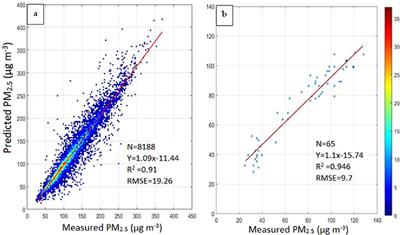
Figure 1. Ten-fold cross-validation of model-predicted PM2.5 concentrations (in µg m−3) with coincident ground-based measurements at (left) 24 h and (right) annual scale. Sampling density is shown by the colour scale.
Download figure:
Standard image High-resolution image3.2. Hotspot analysis
We present the pollution hotspots in Delhi using this ultra-high-resolution data (figure 2). The map also shows the locations of five thermal power plants—Badarpur, Rajghat, Indraprastha, Gas Turbine, and Pragati thermal power plants (that were moved out of Delhi in recent years), 24 industrial sites, three landfill sites, and three waste-to-energy plants.
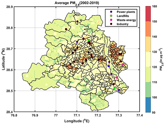
Figure 2. Mean annual PM2.5 exposure during 2002–2019 in Delhi, along with key local emission hotspots. Municipal ward boundaries are also demarcated.
Download figure:
Standard image High-resolution imageSpatial heterogeneity of ambient PM2.5 over Delhi averaged over the entire study period is shown in figure 2, along with the key local emission sources within the city. Several features are noteworthy. First, the mean annual PM2.5 levels over the 18 year period vary in a wide range of 90–160 μg m−3 across the city. The concentrations are relatively lower in the municipal wards at the northern, western, and southern peripheries of the city, while the wards in central and eastern Delhi are among the most polluted. Most of the polluted wards also have a higher population density. Spatial heterogeneity in ambient PM2.5 at a seasonal scale (figure S5) reveals that the hotspots are quite persistent across the peak pollution period of October to June. The pollution level is lowest during the monsoon for obvious reason of washout by monsoon rain (Dey et al 2020). The rainfall pattern, however, varies spatially depending on local urban meteorological factors, and as a result, the hotspots show a different spatial pattern.
Another observation is that PM2.5 exposure does not show a strong gradient as one moves away from the major roads (figure S6), unlike in urban settings in developed countries (e.g. Puett et al 2014). This is because, in Delhi, ambient PM2.5 variation is also modulated by various other local and regional sources. The latest source apportionment study (Sharaf and Sharma 2018) suggests that the transportation sector contributes less than one-third to ambient PM2.5 in Delhi. PM2.5 is observed to be higher in the wards closer to the ring road (www.mapsofindia.com/maps/delhi/delhiroads.htm) and in the wards having landfill sites. Spatial heterogeneity of PM2.5 in Delhi is also weakly influenced by topography (figure S7), as the pollution level in the regions with higher elevation (southern wards) is usually low but similar to values in some pockets in the wards located in the western part of the city.
70% of monitoring stations in Delhi lie in the east and central Delhi (figure S1), where the annual PM2.5 is high. Regions in Delhi where the average annual PM2.5 is low (<110 μg m−3) do not have any ground monitoring. Hence, the city average statistics based on the existing ground monitors may be biased high. Moreover, if Delhi were to expand ground monitoring, the southern, western, and northwestern parts of the city should be covered.
3.3. Inter-annual variations in ambient PM2.5 exposure
We next show the inter-annual variations in ambient PM2.5 in Delhi during 2002–2019 (figure 3). Over the years, PM2.5 did not show any unidirectional trend; rather, it showed ups and downs, with the lowest value observed in 2013. These trends are the manifestation of changes in emission characteristics, meteorology, and Delhi's rapid transition in the last two decades in terms of urban development and policies. For example, the public transportation in Delhi switched to CNG in 2001. Delhi metro rail construction started in 1998, and the first elevated section (Shahdara to Tis Hazari) opened in late 2002. By 2009–2010, a large fraction of the population started using the metro for their daily commute. The expansion and strengthening of the metro network as a major public transport system can be found on the Delhi metro website (www.delhimetrorail.com). The national highway (NH2) became an operation in 2001 (Mehta 2017). During the year 2008, NH8 becomes operational, allowing the movement of traffic from central and south Delhi to Gurugram via shorter routes. The population in Delhi has grown, and as a result, energy use, the number of vehicles, and emissions from various other sources (e.g. waste production, other unorganized sources, etc) have increased.

Figure 3. Spatial patterns of annual PM2.5 (median values in µg m−3 written at the bottom left corner in each panel) were predicted by the RF model in Delhi for the year 2002–2019 at 100 m × 100 m spatial resolution.
Download figure:
Standard image High-resolution imageThe normalized anomaly plots (figure S8) of PM local emission derived from Emissions database for global atmospheric research hemispheric transport of air pollution (EDGAR-HTAP) inventory (Janssens-Maenhout et al 2015), ventilation coefficient (VC, a product of wind speed and planetary boundary layer height) derived from ERA5, and PM2.5 concentration from 2002 to 2018 (emission data was only available till 2018) reveal that the interannual variation in PM2.5 in Delhi is influenced by the combined impact of local emission and regional transport modulated by meteorology. A lower VC (either due to low wind speed creating a calm condition or shallow boundary layer height stabilizing the lower troposphere or both) implies unfavorable conditions for dispersion of pollutants and is expected to increase PM2.5 concentration. On the other hand, higher emission is expected to enhance the concentration. If emission increases and VC decreases, the rise in PM2.5 concentration will be accelerated, while opposite trends in emissions and VC may compensate for each other.
In Delhi, PM2.5 gradually declined from 2002–2004 till 2008–2009, when PM emission showed a lower normalized anomaly (figure S8). From 2006 to 2009, VC increased and perhaps compensated for the impact of rising emissions to keep PM2.5 concentration lower than the 19 year average. PM2.5 concentration again increased in the next few years and decreased to the lowest level in 2013 before reaching a peak in 2016. Crop-waste burning in the upwind states of Punjab and Haryana increased after the implementation of the sub-surface water preservation act in 2009 and was a major reason for the rising concentration during the post-monsoon season post-2009, pulling up the annual average. During this time, local PM emissions also decreased till 2012–2013 and remained similar thereafter. The VC showed a gradual decline between 2013–2014 till 2016, enhancing PM2.5 concentration. After 2016–2017, the major thermal power plants that were operating inside the city either stopped operating or moved out. The GRAP was implemented in 2017 to address the high pollution levels during the post-monsoon to winter seasons. Annual PM2.5 showed a steady decline afterward.
During this period, the spatial heterogeneity also shows a flip-flop pattern. For example, the frequency distribution of PM2.5 concentration (figure S9) shows a wide spectrum across the municipal wards, implying a wide range of variation in PM2.5 exposure across the city. Gradually the spectrum became narrow by 2010 as the range of variation within the city decreased (figure 3). It again shifted to a broader spectrum by 2016–2017, when pollution levels increased by a larger margin in the inner part of the city surrounding the ring roads and in the eastern part. After 2017, PM2.5 consistently showed a decline in the hotspots but showed an increase along the periphery of the city. Interestingly, the peripheral expressway (www.mapsofindia.com/maps/delhi/delhiroads.htm) became operational in 2018, through which all heavy-duty vehicles were diverted. Whether this elevates the observed PM2.5 concentration along the periphery needs to be confirmed with updated emission inventory data and analysis for a longer duration.
3.4. Temporal changes in health burden associated with PM2.5 exposure
In this section, we discuss the changes in mortality and morbidity burden attributable to ambient PM2.5 exposure in Delhi from 2002 to 2019. First, we show the changes in cumulative exposure (figure 4). In 2002, the entire population was exposed to PM2.5 above 100 μg m−3, while in 2019, the entire population was exposed to PM2.5 levels greater than 110 μg m−3. However, clearly, the exposure to very high PM2.5 levels has declined over the years. For example, around 5% population was exposed to PM2.5 greater than 152 μg m−3 in 2002, while no one was exposed to such a high level of pollution in 2019.
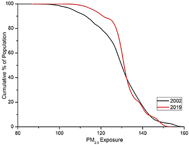
Figure 4. Changes in cumulative population exposure to ambient PM2.5 in 2002 and 2019.
Download figure:
Standard image High-resolution imageIn 2002, 9188 (95% UI: 6241–12 161) deaths in Delhi (table 1) were attributed to ambient PM2.5 exposure, accounting for 10% of all deaths that year. In 2019, 13 652 (95% UI: 11 065–21 899) deaths were attributed to PM2.5, accounting for 8% of all deaths. Though the mortality burden attributable to ambient PM2.5 increased by 49% between 2002 and 2019, its relative share of the total mortality burden has gone down. Similarly, disability-adjusted life-year lost (DALY) attributable to ambient PM2.5 exposure increased by 43.5%, from 317 732 (95% UI: 215 307–426 448) in 2002–456 072 (95% UI: 343 649–571 532) in 2019. Years of life lived with disability (YLD) increased from 38 668 (95% UI: 29 130–65 396) in 2002 to 59 610 (95% UI: 42 213–74 903) in 2019. The age-specific population and baseline mortality values in 2002 and 2019 are shown in figure S10.
Table 1. Total burden (DALYs, YLDs, and Deaths) attributable to ambient PM2.5 exposure in Delhi in 2002 and 2019, and the sensitivity to exposure, baseline mortality, and population remaining unchanged. 95% UIs are shown in parentheses.
| 2002 | 2019 | Constant exposure | Constant baseline mortality | Constant population | |
|---|---|---|---|---|---|
| DALY | 317 732 (215 307–426 448) | 456 072 (343 649–571 532) | 423 134 (324 155–521 296) | 647 473 (494 497–840 234) | 269 544 (117 968–237 103) |
| YLD | 38 668 (29 130–65 396) | 59 610 (42 213–74 903) | 57 575 (41 518–73 269) | 84 703 (57 565–111 628) | 32 419 (24 747–40 010) |
| Deaths | 9,188 (6,241–12 161) | 13 752 (10 065–19 899) | 10 635 (8,496–16 689) | 21 468 (18 822–33 995) | 6,423 (4,561–8,861) |
We find that the mortality burden attributable to ambient PM2.5 exposure in Delhi did not change linearly in the last two decades (figure S11). After a moderate rise between 2002 and 2005, the mortality burden increased rapidly in the next 3 years till 2008. The burden dropped after 2008 and remained more or less constant till 2014–2015, after which it started rising again. These non-linear changes were in response to the changes in exposure and other socio-demographic factors.
Therefore, we separate the relative impacts of individual factors (table 1). If PM2.5 exposure remained constant during this period, the mortality burden would have increased by 15.7% to 10 635 (95% UI: 8496–166 689) due to the changes in population and its age structure and baseline mortality. It means that only additional 3117 deaths can be attributed to the increase in PM2.5 exposure. If baseline mortality remained constant, mortality would have increased to 21 468 (95% UI: 18 822–33 995) in 2019, instead of 13 752. This suggests that a decline in baseline mortality over the years (most likely due to an overall improvement in health infrastructure in the city) prevented an additional 7716 deaths. If the population and aging remained unchanged, mortality would have decreased by 30.1% to 6423 (95% UI: 4561–8861) in 2019. This implies that the population rise in the city caused an additional 7329 deaths during this period. The corresponding numbers for DALY and YLD are also mentioned in table 1.
The relative contributions of various diseases to the overall health burden attributable to PM2.5 exposure in 2002 and 2019 (figure 5) reveal that the general patterns remained similar. IHD had the highest contribution to mortality and DALY in 2002 and 2019; its relative contributions during this period increased from 43% to 50% and from 36% to 43%, respectively. COPD has the second-largest contribution to mortality (decreased from 26% in 2002 and 24% in 2019) and DALY (increased from 215 in 2002 and 24% in 2019), and the highest contribution to YLD burden where its contribution decreased from 60% in 2002 and 56% in 2019. The third highest contribution to the disease burden is stroke, whose contribution to death, DALY, and YLD remained mostly unchanged. For death and DALY, the contributions of T2D and LC also remained unchanged, while that of LRI decreased in this period. After COPD, T2D has the second-largest contribution to the YLD burden in Delhi.

Figure 5. Percent contributions of different diseases to total health burden—death, DALY, and YLD attributable to ambient PM2.5 in Delhi for (top panel) 2002 and (bottom panel) 2019.
Download figure:
Standard image High-resolution image
3.5. Exposure reduction targets for Delhi in 2030
We finally report the exposure reduction targets for the adult population in Delhi to achieve the SDG3.2 target. If ambient PM2.5 exposure decreases to 20 μg m−3 in 2030, the mortality burden of IHD attributable to ambient PM2.5 exposure will decrease by one-third from 5 083 in 2015 (table S3) to 3 388 in 2030. To reduce the burden of stroke, COPD, LC, and T2B by one-third in 2030, the corresponding exposure targets should be 41, 53, 29, and 23 µg m−3, respectively. Exposure targets for different diseases are not uniform because the RRs are different at a given exposure for different diseases (Murray et al 2020). If ambient PM2.5 exposure decreases below the World Health Organization's (WHO) first interim target (IT-1) of 35 μg m−3 in 2030, the total mortality burden attributable to PM2.5 in Delhi will decrease by one-third relative to the 2015 burden.
Even if Delhi cannot reduce the exposure below WHO IT-1, exposure below 69, 91, and 42 µg m−3 in 2030 will at least maintain the same burden as of 2015 for stroke, COPD, and LC, respectively. However, to maintain the same burden for IHD and T2D, exposure needs to be reduced to 24 and 35 µg m−3. We note that the burden of IHD, stroke, COPD, LC, and T2D are higher for the older population (table S3). Hence, the projected age-distributed population also plays a role in impacting the exposure targets set for 2030 in Delhi. Also, the differences in baseline mortality are another factor for different exposure targets to achieve similar burden reduction goals. To summarize, achieving the national ambient air quality standard of 40 μg m−3 first and then the WHO IT-1 would reduce the health burden associated with air pollution considerably in Delhi in the coming years.
4. Discussion and conclusions
In this work, we develop and present an ultra-high resolution (100 m) PM2.5 exposure database for the megacity Delhi using machine learning. Our model can predict daily and annual PM2.5 at such high resolution with a high level of accuracy. This is one step forward from the current efforts of mapping PM2.5 levels at a 1 km spatial scale nationally (Dey et al 2020) for air quality management at a hyperlocal scale. Our methodology can be applied to extend PM2.5 monitoring in Delhi at such high resolution for recent years and be adopted for any other polluted city in India. This data can be used to evaluate the performance of the air quality early warning system in forecasting PM2.5 and its spatial pattern at 400 m resolution in Delhi (Jena et al 2021). We also note that the true model performance for the years without or with limited ground data cannot be assessed. Since the model can predict PM2.5 in a wide range based on the predictor variables, we feel that the data is robust enough for further interpretation.
We perform a sensitivity analysis to understand the differences in health burden due to the improvement in exposure data. We find that the DALY, YLD and mortality burdens in Delhi were 6%, 10% and 10%, respectively, higher with 100 m exposure data than that with 1 km exposure data in 2002 (figure S12). The corresponding differences in 2019 were 3.2%, 3.4% and 3.1%, respectively. A lower difference in 2019 than in 2002 is primarily due to reduced spatial heterogeneity in exposure (figure 3). It is not possible to evaluate the accuracy of the estimated burden in India or in any other country due to the lack of direct evidence. Therefore, we cannot comment whether the estimated burden using 100 m scale exposure data is better than the burden with 1 km scale exposure data. In states or cities where the population distribution is more heterogenous, having such high-resolution exposure data will make a larger difference in the estimated health burden of air pollution. Many cities in India have either a single ground monitor or a handful of monitors. Exposure assessment in those cities relying on ground monitors would result in a larger uncertainty. Machine learning models can be applied to generate spatially resolved estimates of PM2.5 in those cities for better exposure assessment. Estimation of health burden attributable to ambient PM2.5 may be impacted by exposure misclassification if the population is exposed to high levels of household PM2.5 (McDuffie et al 2021). Household PM2.5 exposure in India is important, but it is negligible in Delhi, and therefore, we only focused on ambient PM2.5.
We use the RF model in our present work. Our objective in this study was to explore if PM2.5 can be mapped at such high spatial resolution in the megacity Delhi reliably using machine learning and if yes, then use the information for air quality management at municipal ward level and estimating health burden. Since the model performance seems to be adequate, we did not check other machine-learning algorithms (e.g. support vector machine, XGBoost, etc.). A comparative assessment of various machine learning algorithms in predicting PM2.5 at hyperlocal scale in Indian cities could be a topic for future work. We also note that technically the same method can be used to map PM2.5 at even finer spatial scale, but the model may not be adequately trained to capture the spatial heterogeneity at finer resolution. The present scale is good enough to derive the information at municipal ward level for administrative purpose.
Based on the air quality monitoring guidelines of the CPCB, Delhi requires at least 77 monitoring stations, 37 more than the existing continuous monitoring sites. Our data provides the spatial coverage required to track air quality at the municipal ward level within the city, including regions currently devoid of any ground monitoring. We emphasize that PM2.5 monitoring sites expanded in Delhi only after 2017 and did not allow an understanding of long-term changes in PM2.5 levels in response to various policies that were undertaken by the GoI. This gap can be filled by using our data. Since there were no ground measurements prior to 2009, it is not possible to quantify uncertainty in estimates during that period. Since the model predicts PM2.5 reasonably well across a wide range of levels over multiple years, we believe that the estimates would be robust during the period 2002–2009 as well.
Our analysis on the health burden shows that the increase in mortality and morbidity burden attributable to PM2.5 exposure in Delhi over the last two decades has been influenced more by the changing age-distributed population and baseline mortality than the exposure itself. In fact, a decline in baseline mortality of the NCDs that are medically linked to air pollution over the years helped Delhi to compensate for the impact of the rising population on the disease burden. This could be a lesson for other polluted states in India that an overall improvement in health infrastructure, in addition to efforts to reduce emissions of air pollutants, can minimize the health burden of air pollution faster. Also, the change in health burden attributable to air pollution is not persistent as often perceived. In fact, in Delhi, we find periods when health burden of air pollution did not increase or even reduced.
We find that the relative proportions of diseases to health burden mostly remained similar in the last two decades in Delhi. For getting considerable health benefits by reducing the mortality burden of air pollution by one-third in 2030 relative to that in 2015, a larger reduction in PM2.5 exposure is required for IHD, LC, and T2D compared to COPD and stroke. We find that achieving the WHO IT-1 in 2030 would help Delhi meet the SDG3.4 target. In a sustainable development scenario defined in Purohit et al (2019), ambient PM2.5 exposure in Delhi is expected to reduce to 90 μg m−3 in 2030, which will only allow maintaining the COPD burden same as in 2015. Therefore, stronger actions are required, that too beyond the NCAP target year to achieve considerable health benefits in the future. This is only possible by strengthening inter-state coordination in implementing a clean air action plan in a cost-effective and systematic way. Priority may be given to the sources that co-emit air pollutants and climate pollutants and to the sectors that emit species that have a stronger impact on health (Joshi et al 2022).
Key conclusions of our study are as follows:
- Machine learning can be reliably used to assess exposure at hyperlocal scale for urban areas with moderately dense ground network.
- Exposure estimates at scale finer than 1 km increases the health burden attributable to ambient PM2.5 in Delhi by 6%–10%.
- In Delhi, mortality burden of air pollution increased by 47.9% from 2002 to 2019, but only 16% of this rise can be attributed solely to the change in PM2.5 levels. Hence, the changes in health burden attributable to air pollution needs to be interpreted in terms of socio-demographic factors in policy framing.
- If Delhi reduces PM2.5 exposure to the WHO IT-1 by 2030, it will meet the SDG3.4 goal of reducing air pollution health burden by one-third relative to 2015 level.
Acknowledgments
The work is supported by a grant under 'Delhi cluster-Delhi research implementation and innovation (DRIIV)' funded by the office of the Principal Scientific Adviser to the Government of India (Prn.SA/Delhi-Hu/2018(C)) and a grant from Science and Engineering Research Board, GoI under SUPRA scheme. S.D. acknowledges the support from IIT Delhi for the Institute Chair fellowship. CPCB data are available from the data portal www.cpcb.nic.in. AOD data are archived at NASA LP DAAC. We thank the reviewers for providing comments that helped improve the manuscript.
Data availability statement
The data that support the findings of this study are available upon reasonable request from the authors.
Supplementary data (2.3 MB DOCX)