Subseasonal reversals of winter surface air temperature in mid-latitude Asia and the roles of westward-shift NAO

Global surface air temperature (SAT) records exhibit a remarkable long-term warming trend. However, in recent winters, mid-latitude Asia (MA, 35°–58° N, 65°–120° E) has suffered more frequent extreme cold surges (Mori et al 2014) and SAT reversals (Li et al 2022b), which have serious negative consequences for human health, ecological systems and livestock husbandry (Li et al 2022a). During the 2015/16 boreal winter, an unusually warm period was observed over East Asia in early winter, and an extreme cold wave was recorded in mid–late January, with SAT differences between early and late winter of up to 6.5 °C (Geng et al 2017). The winter of 2020/21 showed a significant reversal from cold to warm in East Asia, with a maximum SAT difference of 18 °C (Yang et al 2022). This subseasonal reversal of SAT can end the dormancy period of crops, freeze vegetables and cause damage to infrastructure (IPCC 2012). In addition, the subseasonal SAT reversals also represent a challenge in the context of short-term climate prediction (Li et al 2020). Therefore, subseasonal variations in the spatial and temporal distribution of SAT should be investigated to improve its predictability.

Previous studies have revealed that the variation of winter SAT anomalies over MA is largely controlled by the large-scale atmospheric circulation at mid–high latitudes (Li et al 2022a). Two critical semi-permanent atmospheric systems over the Eurasian continent play important roles in linking climate variations in the Arctic and Eurasia: the Siberian high (SH) and the Ural blocking high (UBH) (Cohen et al 2001, Cheung et al 2012). The frequency of cold-wave conditions in East Asia is positively correlated with the intensity of the SH (Ding et al 1990). An enhanced SH may contribute to an outbreak of cold-wave events over MA via related changes in radiation conditions and heat budgets (Cohen et al 2001, Gong and Ho 2002). The quasi-biweekly warm Arctic–cold Eurasia anomaly will be stronger when associated with the UBH (Luo et al 2016). In addition, the effects of the development and decay of the UBH are not limited to the direction of the trough downstream—they are also strongly linked to the evolution of the SH and cold-wave events (Peng et al 2022). Persistent strengthening of the UBH and SH and northerly winds ahead are key drivers of enhanced cold advection (Zhou et al 2009, Liu et al 2019), which can lead to the continued presence of a cold anomaly in MA. In contrast, when the UBH and SH show subseasonal out-of-phase changes during the winter, a corresponding reversal of SAT also occurs (Yan et al 2022, Yu et al 2022).

The North Atlantic Oscillation (NAO) has long been recognized as a key factor in the winter SAT variation over Eurasia (Trigo et al 2002). Previous studies have also found that the NAO can influence SAT variation by regulating the frequency of cold air bursts (Hurrell and Van Loon 1997). In the positive phase of the NAO, the strengthened westerly wind field guides warm air to MA, resulting in a warm anomaly (Trigo et al 2002). However, research has also shown that the effects of the NAO are complex and are related not only to the NAO phase but also to its spatial distribution. Different combinations of the NAO and the East Atlantic pattern or the Scandinavia teleconnection (SCAND) correspond to different temperature, precipitation, and wind speed responses across Europe (Comas-Bru et al 2014). Eastward shift of the NAO could affect the number of deep cyclones, near-surface air temperature and turbulent surface heat flux (Jung et al 2003). In the summer, this shift also favors rainfall over East Asia during the positive phase (Sun and Wang 2012, Du et al 2020).

Previous studies have focused on the influence of atmospheric circulations, such as the NAO, SH and UBH on average winter SAT anomalies over MA, and the mechanisms via which these influences occur. However, SAT in MA exhibits significant subseasonal variations in winter (Yang and Fan 2022, Li et al 2022a), which may lead to extreme climate events. For example, the significant SAT reversal from cold to warm in winter 2020 was conducive to the occurrence of sandstorms in the following spring (Yin et al 2022). Recent studies have demonstrated that a rapid subseasonal reversal of NAO phase can lead to SAT reversal (Geng et al 2017), but the relationship between changes in the spatial distribution of the NAO and SAT anomalies remains unclear. In this article, we aim to highlight the subseasonal variability of SAT in MA and associated atmospheric circulation, and to further clarify the role of the spatial distribution of the NAO.

2.1. Data

2.2. Methods

Season-reliant empirical orthogonal function (S-EOF) analysis was used in this study to assess the year-to-year variation of winter SAT in MA, and its subseasonal evolution in particular. The derived spatial patterns for each S-EOF mode contained two sequential patterns representing the subseasonal evolution of the SAT. They share the same yearly value in their corresponding normalized time series of the standardized principal component (PC) (Wang and An 2005).

Horizontal wave activity fluxes (WAF) were computed to analyze the propagation of Rossby waves, based on the equations generalized by Plumb (1985):

$$\begin{equation*}{\text{WAF}} = p\cos \varphi \left\{ {\begin{array}{*{20}{c}} {{{v^{^{\prime} }}^2} - \frac{1}{{2\Omega \sin 2\varphi }}\frac{{\partial \left( {v^{^{\prime} }\Phi ^{^{\prime} }} \right)}}{{\partial \lambda }}} \\ { - u^{^{\prime} }v^{^{\prime} } + \frac{1}{{2\Omega \alpha \sin 2\varphi }}\frac{{\partial \left( {u^{^{\prime} }\Phi ^{^{\prime} }} \right)}}{{\partial \lambda }}} \end{array}} \right\}\end{equation*}$$

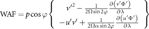
where p is air pressure, u and v represent zonal and meridional winds, Ф is geopotential height, Ω is the Earth's rotation rate, α is the Earth's radius, and ϕ and λ are latitude and longitude, respectively.

The daily evolution of area-average SAT anomalies over MA (SAT_MA) in winters over the period 1979–2021 showed that the average subseasonal reversal point was 16 January (not shown). For example, the winter of 2020 showed a persistent cold anomaly before 16 January and a persistent warm anomaly after this date, with an average shift in SAT_MA from −2.5 °C to 1.5 °C (figure S1). The abrupt change characteristic of the SAT reversal was clearly evident in the latitude–time profile (figure S2), indicating that 16 January was the time point at which the reversal occurred. Winter can therefore be divided into two periods: early winter (1 December to 16 January) and late winter (17 January to 28 February).

The first two leading S-EOF modes of early and late winter SAT in MA were separable and well distinguished from each other. In the first mode, a consistent SAT anomaly was observed for early and late winter (figure S3). This means that the whole winter will be warmer or colder than usual. In contrast, in the second mode, the SAT exhibited a reversal between early and late winter (figures 1(a) and (b)). The correlation coefficients between the standardized second principal component (PC2) and SAT_MA for early and late winter were 0.79 and −0.48, respectively, both of which were higher above the 95% significance level. Based on PC2 and daily SAT_MA, the winters during 1979–2021 can be divided into three categories: 'warm to cold' reversal (R_W–C), 'cold to warm' reversal (R_C–W) and 'no reversal' (NR). R_W–C/R_C–W were defined as the winters for which the standardized PC2 was above 1/below−1 standard deviation and the SAT_MA in early and late winter was reversed (figure 1(c)). For R_W–C and R_C–W, there was a marked opposite in SAT_MA between early and late winter (figure 1(d))—a consistent finding that was not caused by extreme values—while NR showed a small fluctuation (figure 2(a)). Calculations of R_W–C minus R_C–W showed that SAT_MA exhibits a persistent warm anomaly in early winter and a persistent cold anomaly in late winter. However, the intensity of the cold anomalies in R_W–C and R_C–W was more significant than that of the warm anomalies; the site OBS also showed the same results (figure 2(b)).

Zoom In Zoom Out Reset image size

Zoom In Zoom Out Reset image size

In the R_W–C winter, SAT over MA exhibited a positive anomaly (SAT_MA = 1.36 °C) in early winter and a negative anomaly (SAT_MA = −1.94 °C) in late winter (figures 3(a) and (b)). In contrast, R_C–W showed a reversal from negative to positive (−1.93 °C in early winter and 1.02 °C in late winter) (figures 3(c) and (d)). The spatial distribution of SAT was not the same for early and late winter in both R_W–C and R_C–W. In early winter, the SAT anomaly showed a consistent variation throughout the whole of Eurasia, with maximum values appearing in the northwest of MA (figures 3(a) and (c)). However, in late winter, the SAT anomaly was characterized by a dipole pattern similar to warm Arctic–cold Eurasia (Zhang et al 2021), with two anomaly centers over the Arctic and MA (figures 3(b) and (d)). The maximum value of the SAT anomaly occurred in the center of MA. Differences in the spatial distribution between early and late winter SAT anomalies were also observed in the site OBS data (figure S4), which suggested that different physical mechanisms may modulate the changes of SAT in early and late winter. In addition, in reversed winters, late winter SAT_MA was often significantly correlated with SAT in eastern China, which means that if the reversal in late winter cannot be predicted, the signal in eastern China may also be missed.

Zoom In Zoom Out Reset image size

The same criteria were used to analyze the winters for each CMIP6 model, and the SAT_MA values in early and late winter for the R_W–C and R_C–W were calculated (figure 3(e)). For all CMIP6 models, the average difference between early and late winter SAT_MA was found to be 3.22 °C for R_W–C and −3.40 °C for R_C–W. These values are close to those from the ERA5 reanalysis data (3.30 °C and −2.95 °C). However, the ability of different models to capture SAT_MA reversals varies significantly, with the best-performing models able to capture 11 winters and the worst-performing models managing to capture only one (table S1). The vast majority of models were able to capture SAT_MA reversals of five winters or more, but only eight models were able to capture a comparable proportion of reversed winters to ERA5 (i.e. >10). In other words, although every model could capture the reversal of SAT_MA, the number of years of reversal captured was generally small and the simulation ability varies greatly between models.

Corresponding to the reversal of SAT_MA, the key atmospheric circulation characteristics from the lower to the upper troposphere during R_W–C and R_C–W also differ significantly between early and late winter (figures S5 and S6). The differences in atmospheric circulations between R_W–C and R_C–W winters were very similar to the spatial distribution of R_W–C and R_C–W, confirming the need to further analyze the differences between R_W–C and R_C–W (figure 4). For ease of description, the subsequent analyses were based on the difference between R_W–C and R_C–W (i.e. R_W–C minus R_C–W).

Zoom In Zoom Out Reset image size

In early winter, the zonal wind at 200 hPa exhibited a positive/negative pattern of anomalies from north to south over the North Atlantic (figure 4(a)), which corresponded well to the geopotential height anomaly at 500 hPa. The strong WAF over the North Atlantic coincided with a meridional dipole pattern in the geopotential height. In addition, the WAF propagates eastward from the Atlantic to MA, exciting a zonal wave train pattern characteristic of the negative phase of SCAND (figure 4(a)). The eastward extension of the North Atlantic jet stream (NAJS) enhanced the anticyclonic circulation anomaly over northern China (Du et al 2020) and, as one center of SCAND, blocked the southward movement of cold polar air, resulting in a warm anomaly in MA. At this point, SCAND was the dominant middle troposphere teleconnection that affected early winter SAT, and the correlation coefficient between PC2 and SCAND (CC = −0.76) was significantly higher than that of UBH (CC = −0.25) (figure 5(a)). The SLP anomalies exhibited an NAO-like pattern, the positive anomaly showing two centers in the Atlantic Ocean and Western Europe, but the former was stronger (figure 4(c)). The negative anomaly was significantly stronger than the positive anomaly, and its eastward extension into Siberia led to a weakened SH. The accompanying strong southwest wind over Eurasia prevented the southward movement of cold air. Therefore, the co-regulation of the eastward extension of the NAJS, the negative phase of SCAND, the weakening of UBH and SH, and the southerly winds near the surface led to the positive SAT anomaly in early winter.

Zoom In Zoom Out Reset image size

In late winter, the atmospheric circulation was significantly different from those observed in early winter. The NAJS receded significantly westward relative to its position in early winter. The abnormal easterly wind over Asia shifted northward to the north of MA and intensified (figure 4(b)). This corresponded to a significant strengthening of the UBH and brought cold polar air to MA. SAT shifts from a warm anomaly in early winter to a cold anomaly in late winter, resulting in the reversal of SAT_MA. WAF manifests primarily as meridional transport, corresponding to a significant enhancement of the meridional gradient of the atmospheric circulation in the middle troposphere. Cold advection in the Arctic and the warm advection in Eurasian led to a meridional dipole anomaly in SAT in late winter. In addition, SCAND was no longer the dominant mode in late winter, and the correlation coefficient with PC2 was only 0.04 (figure 5(c)). The UBH became the dominant middle troposphere atmospheric system affecting SAT_MA (CC = 0.54). This finding is also supported by the results of a previous study, which demonstrated that the formation of dipole patterns over the Arctic–Eurasia region may be related to the UBH (Li and Fan 2022b). Near the surface, a significantly enhanced SH is accompanied by strong northerly winds formed over Eurasia (figure 4(d)), bringing cold advection to MA.

In short, the reversal of SAT_MA was associated with changes in the atmospheric circulation anomalies in late winter relative to early winter. However, it is noteworthy that the phase of the NAO did not show the expected opposite sign, but the spatial distribution of the NAO in late winter was different from that of early winter. In late winter, the negative northern center of action was weakened, while the positive southern center shifted westward and strengthened significantly.

This reversal of the atmospheric circulation can also be reproduced by the CMIP6 models. Taking the SH as an example, in more than 85% of CMIP6 models, the SH index showed the opposite sign when the SAT_MA was reversed (figure S7). However, the model simulations underestimated the strength of the SH, especially in late winter. Only two models were able to match the differences between R_W–C and R_C–W that were observed in the ERA5. Moreover, CMIP6 models could not simulate the asymmetry of SH intensity in early and late winter. Therefore, although CMIP6 models can simulate the sign reversal of the SH, its intensity is poorly simulated.

The SAT_MA reversal was associated with significant differences in atmospheric circulation. Between the early and late winter, correlation coefficients between PC2 and UH, SCAND, V850 and SH were of the opposite sign, but were all positive between NAO and PC2, which instead of the expected contrary (figure 5(a)). This raises the question of why the same NAO phase causes SAT reversal. In addition, the correlation between PC1 (persistent SAT anomaly over MA) and the NAO also shows the same positive sign in early and late winter (figure 5(c)). Why are the effects of the NAO on SAT_MA so diverse? And by what mechanism do these effects occur?

Previous studies have shown that SAT is sensitive not only to the phase of the NAO, but also to the exact location of the NAO centers (Castro-Díez et al 2002). Therefore, it was speculated that changes in the spatial distribution of the NAO lead to the different SAT_MA responses. Some studies have demonstrated that the southern center of the NAO shows obvious meridional position difference, sometimes shifting more than 35° in longitude (Peterson et al 2003). This significant east–west shift may account for the different effects of the NAO. Hereafter, the NAO with its southern center shifting westward and located over the North Atlantic is referred to as NAO_W (figure 5(b)), south center shift eastward and located over Western Europe is referred to as NAO_E (figure 5(d)). The northern centers of both NAO_W and NAO_E are located near Iceland, which is the average location of the climate. The partial correlation between PC2 and the NAO_W (0.20 in early winter, 0.58 in late winter) was significantly higher than that of the NAO_E (0.06 in early winter, −0.13 in late winter), especially in late winter, indicating that the reversal of SAT_MA was largely due to the NAO_W. In contrast, the persistent SAT anomalies were mainly affected by the NAO_E, and the partial correlation between PC1 and the NAO_E (0.40 in early winter, 0.38 in late winter) was higher than that of the NAO_W (–0.16 in early winter, −0.10 in late winter). Regression of SLP onto PC1 and PC2 also confirmed the different responses of SAT to different spatial distributions of the NAO (figures 5(b) and (d)), that is, persistent SAT_MA corresponds to the NAO_E and SAT_MA reversal corresponds to the NAO_W.

In winters with opposite NAO phases in early and late winter, SAT was influenced by both the phase and spatial distribution of the NAO, and most of them were weak or of unclear type in early or late winter (figure not shown). Therefore, this paper focuses more on the effect of the spatial distribution of the NAO and does not consider winters with reversed NAO phases (table S2). Under the premise that the NAO phase was unchanged in early and late winter, winters were divided into four categories according to the relative strength of NAO_W and NAO_E index: WIN-W (NAO_W for early and late winter), WIN-E (NAO_E for early and late winter), WIN-WE (NAO_W for early winter and NAO_E for late winter) and WIN-EW (NAO_E for early winter and NAO_W for late winter). Of these four winter types, SAT reversal occurs more often during WIN-W and WIN-EW, both of which show the NAO_W in late winter. Nine SAT_MA reversal winters showed the same NAO phase in early and late winter, eight of which were WIN-E or WIN-WE (tables S3(a) and (b)). SAT_MA reversals were observed in more than 60% of WIN-W and WIN-EW winters, and most positive (negative) NAO winters exhibit R_W–C (R_C–W). In some WIN-W and WIN-EW winters, such as 1984 and 2011, there was no change in the sign of SAT_MA between early and late winter, but the degree of variation in SAT_MA was large and was comparable with that of reversal winters. In contrast, all of the WIN-E winters and half of WIN-WE winters exhibited persistent SAT_MA anomalies (tables S3(c) and (d)), and most positive (negative) phase winters show continuous warm (cold) anomalies.

In WIN-W (positive phase minus negative phase) winters, most of which showed an SAT_MA reversal, the atmospheric circulation showed similar characteristics to those of SAT_MA reversal years (figure 6). The increasing zonal wind and eastward extension of NAJS in early winter favors barotropic kinetic energy conversion to seasonal kinetic energy, thus providing adequate kinetic energy for cyclonic eddy growth (Du et al 2020). Warm and moist air in front of the trough transported from the North Atlantic Ocean to Eurasia, and the air column over Siberia was heated, causing the weakening of the SH. In late winter, the NAJS westward receded, reducing the eastward movement of the cyclone, which was not conducive to the transport of warm and moist air over the North Atlantic. In addition, the ridge near the Ural Mountains facilitated the formation of the blocking, and the anomaly anticyclone enhanced the northerly surface winds and lead to cold air accumulation over Siberia, resulting in an enhanced SH (Ma et al 2018). The geopotential height in the middle troposphere changed from a positive anomaly over Eurasia to an Arctic–Eurasia meridional distribution with the strengthening of the UBH. The SH showed a negative anomaly in early winter and a positive anomaly in late winter, resulting in the wind anomaly over MA changing from a southerly wind before the trough to a northerly wind before the ridge. Together, these variations led to a very significant subseasonal reversal of SAT_MA from a positive anomaly (SAT_MA = 2.02 °C) in early winter to a negative anomaly (SAT_MA= −2.14 °C) in late winter (figure 6). The spatial distribution of SAT anomalies was also consistent with that of SAT_MA reversal winters (figure 3). For WIN-EW, the atmospheric circulation characteristics were largely the same as those of WIN-W, with SH, UBH and surface wind reversals in early and late winter, leading to the reversal of SAT_MA (5.23 °C in early winter and −0.84 °C in late winter) (figure S8).

Zoom In Zoom Out Reset image size

In WIN-E, which showed a persistent SAT_MA in most winters, the characteristics of atmospheric circulation in early winter lasted into late winter (figure 7). A continuous eastward extension of the NAJS resulted in negative anomalies of the UBH and SH and were stronger in late winter. Persistent and strengthened southerly winds dominated Eurasia, causing more significant SAT anomalies in late winter. These persistent atmospheric circulations resulted in a warm anomaly over MA throughout the whole winter (1.51 °C in early winter and 1.67 °C in late winter) (figure 7). The warm anomaly in early winter was mainly located over northeast MA, and in late winter was observed over Europe and northwest MA. For WIN-WE winters, there was no change in sign for SAT_MA and an increase from 0.54 °C in early winter to 2.80 °C in late winter was observed (figure S9).

Zoom In Zoom Out Reset image size

In this study, winter SAT reversal over MA was studied at the daily scale. Season-reliant empirical orthogonal function analysis of early and late winter showed that SAT reversal over MA occurred in the second mode (figures 1(b) and (d)). Persistent SAT_MA anomalies and significant changes in sign between early and late winter were observed for both R_W–C and R_C–W (figure 2). The characteristics of the atmospheric circulations for R_W–C minus R_C–W showed clear differences between early and late winter. In early winter, the NAJS extended eastward and the middle troposphere was largely controlled by SCAND. The lower troposphere was characterized by a negative SH anomaly and a strong southerly wind anomaly (figures 4(a) and (c)), leading to a positive SAT_MA anomaly. In late winter, the NAJS moved westward, and the middle troposphere was mainly controlled by the UBH and exhibited an Arctic–Eurasia meridional distribution. The lower troposphere showed a significant positive SH anomaly and a northerly wind anomaly (figures 4(b) and (d)), resulting in a negative SAT_MA anomaly. In combination, the above factors led to the reversal of SAT between early and late winter (figures 3(a)–(d)).

More importantly, the relationship between the spatial distribution of the NAO and the reversal of the SAT anomaly was explored. It was found that SAT reversal was more likely to occur when the south center of NAO shifts westward, and when the south center of NAO shifts eastward the SAT will be persistent (figures 5(b) and (d)). In this article, winters were divided into four categories: WIN-W, WIN-E, WIN-WE and WIN-EW. In WIN-W and WIN-EW, changes in atmospheric circulation were similar to those observed in SAT_MA reversal winters: between the early and late winter SH, the UBH and surface wind reversals were observed, leading to the reversal of SAT_MA (figures 6 and S8). In WIN-E and WIN-WE, the atmospheric circulation in early winter lasted into late winter (figures 7 and S9). Further strengthening of the UBH and SH in late winter resulted in a continuously increasing warm anomaly over MA.

The results presented here show that different NAO spatial distributions correspond to different atmospheric circulations in early and late winter, but how NAO causes the change of atmospheric circulation is worthy of further study. The relationship between SAT reversal and the NAO has also been analyzed based on the CMIP6 models, but the relationship is not well demonstrated. In 80% models, WIN-W and SAT reversals co-occurred in less than three winters. There are two possible reasons for the discrepancy between the CMIP6 models and ERA5 results. First, the models themselves are poor at simulating SAT reversal. Second, the NAO prediction skill of the models is limited to subseasonal timescales, particularly in terms of their spatial distribution (Johansson et al 2007). The frequency of SAT_MA reversal is closely related to SAT anomalies in eastern China, so it is of great significance to study and predict the reversal of SAT_MA. However, the effect of global warming on SAT_MA reversal is unclear, and the relationship between the two deserves continuous attention and research. In addition, the effects of forcing factors on SAT_MA were not considered, though SAT_MA is known to be affected by factors such as snow cover (Wu and Chen 2016), North Atlantic sea surface temperature (Chen et al 2021) and Arctic sea ice (Mori et al 2014). At the same time, the NAO is also affected by forcing factors, such as the El Niño-Southern Oscillation (Zhang et al 2015), snow cover (Deser et al 2004) and sea ice (Screen et al 2013). Therefore, the relationship between SAT and the NAO is complicated. In short, more factors need to be considered to fully understand the reversal of SAT anomalies over Eurasia during early and late winter and the relationship between these reversals and the spatial distribution of the NAO.

This research is supported by the National Natural Science Foundation of China (Grant No. 41991283).

Daily 2m temperature and sea level pressure can be obtained from https://cds.climate.copernicus.eu/cdsapp#!/dataset/reanalysis-era5-single-levels?tab=form. Daily geopotential height at 500 hPa, winds at 850 hPa and zonal wind at 200 hPa can be obtained from https://cds.climate.copernicus.eu/cdsapp#!/dataset/reanalysis-era5-pressure-levels?tab=form. The Global Historical Climatology Network daily average SAT (GHCNd) can be obtained from www.ncei.noaa.gov/data/global-historical-climatology-network-daily/access/. The simulation data of 46 CMIP6 models are available from https://esgf-node.llnl.gov/search/cmip6/. Daily NAO index can be obtained from www.cpc.ncep.noaa.gov/products/precip/CWlink/pna/nao.shtml. Monthly SCAND index can be obtained from www.cpc.ncep.noaa.gov/data/teledoc/scand.shtml.

All data that support the findings of this study are included within the article (and any supplementary files).

Yin Z C designed the research. Song X L, Zhang Y J and Yin Z C performed research. Song X L prepared the manuscript with contributions from all co-authors.

The authors declare no conflict of interest.