Gaussian copula modeling of extreme cold and weak-wind events over Europe conditioned on winter weather regimes

Temperature is well established as the main weather driver of electricity demand. We use hourly 2 m temperature and 10 m wind data from the ERA5 reanalysis [36], produced by the European Centre for Medium-Range Weather Forecasts. The data are provided on a regular latitude-longitude grid at $0.25^\circ\,\times\,0.25^\circ$, and the period covered in this work is from 1979–2021. We compute daily minimum temperatures from these hourly data. Wind speeds are calculated from the eastward (u) and northward (v) components at an hourly frequency and then aggregated to daily maximum values. Daily minimum wind speeds are usually close to zero, but low daily maximum values represent well conditions for poor wind power generation. Despite the good coverage and long records, and the fact that ERA5 outperforms other global reanalyses frequently used in the literature, it is discouraged to use global reanalyses to estimate mean winds because of the uncertainty in these data [37].

Atmospheric circulation is well known for its variability at multiple time scales being reflected in weather patterns and circulation systems. These WRs are quasi-stationary large-scale circulation patterns [38]. They typically persist for 6–10 days, are spatially well defined, and limited in number. The understanding of the causes of their recurrence, persistence, and transition is crucial for medium-range, subseasonal, and seasonal-to-interannual climate prediction [27, 29], as they influence the weather at the surface and, subsequently, the renewable power generation and electricity demand [12, 31, 39].

WRs are obtained here by applying the k-means algorithm with four centroids on geopotential height at 500 hPa (Z500) data [26, 27]. The algorithm leads to four winter regimes in the Euro-Atlantic area (27^∘N–81^∘N, 85.5^∘W–45^∘E), and has been adopted by other authors [e.g. 11, 12]. The Z500 fields of the obtained regimes are similar, although not identical, to the teleconnection patterns defined by the National Oceanic and Atmospheric Administration, and can be interpreted as the negative and positive phases of the NAO, the Atlantic Ridge (AR), and the Scandinavian blocking (SCAND) (see figure 1 in the supplementary material). We will therefore use these names to refer to the four WRs. Moreover, it has been shown that temporal sub-sampling [27] and the use of different reanalysis data [11, 12] do not change the spatial structure of the regimes nor the optimal partition ($k\,=\,4$).

The classification method consists of two steps. First, a cosine weight as a function of latitude is applied to the Z500 data and the first fourteen empirical orthogonal functions are computed. The associated principal components (PCs) were used as coordinates of a reduced phase space. Then, the PCs are clustered into four groups with the K-means algorithm, choosing 30 random starts and a maximum of 100 iterations. Every daily map is assigned to a centroid based on its closest Euclidean distance. The number of regimes, $k\,=\,4$, corresponds to the most robust regime partition during winter months [26].

In this study, we use logistic regressions to classify cold and weak-wind events. The predictors consist of two sets of indicator variables, one for the five winter months and one for the four WRs. The variables in each group are dichotomous and take only the values 1 or 0. The univariate distributions will later be used in the copula framework to estimate the joint probabilities.

Logistic regressions are widely used linear models for binary classification. Let Y be the binary outcome variable indicating failure or success with ${0, 1}$. Then, p stands for the probability of a positive event, i.e. $p\,=\,P(Y\,=\,1)$. The mathematical expression of the logit function is:

$$\begin{equation} logit(\,\textit p) = log\left(\frac{\textit p}{1-\textit p}\right). \end{equation} \tag{ 1 }$$

It is assumed that the logit transformation of the outcome variable has a linear relationship with the predictor variables: $x_1, x_2, \ldots, x_k$. Then $\beta_0, \beta_1, \ldots, \beta_k$ are the parameters estimated via the maximum likelihood method when performing a logistic regression of Y on $x_1, x_2, \ldots, x_k$:

$$\begin{align} logit(\,\textit p) = log\left(\frac{\textit p}{1-\textit p}\right) = \beta_0 + \beta_1 \textit x_1 + \ldots + \beta_\textit k \textit x_ \textit k. \end{align} \tag{ 2 }$$

We are usually interested in predicting the probability that a particular sample belongs to a particular class. The formula of the probability $P(Y\,=\,1)$ is:

$$\begin{equation} p = \frac{e^{\beta_0 + \beta_1 \textit x_1 + \ldots + \beta_\textit k \textit x_\textit k}}{1+e^{\beta_0 + \beta_1 \textit x_1 + \ldots, \beta_\textit k \textit x_\textit k}} = \frac{1}{1+e^{-(\beta_0 + \beta_1 \textit x_1 + \ldots + \beta_\textit k \textit x_k)}}. \end{equation} \tag{ 3 }$$

Our goal is to establish a methodology for modeling the probabilities of co-occurrence of cold temperatures and weak winds. However, estimating joint densities is not an easy task since only a few non-Gaussian families are defined, and non-parametric estimation is demanding. Nonetheless, density estimation in one variable is relatively easy, given that many convenient families exist (e.g. logistic, exponential, uniform) and that the non-parametric approach is efficient and accurate. The copulas framework for modeling multivariate distributions provides a flexible representation and separates the univariates from their true nature of dependence.

In the field of probability theory and statistics, a copula function $C:[0, 1]^n \rightarrow [0, 1]$ is defined as a multivariate distribution:

$$\begin{equation} C(u_1,u_2,\ldots.,u_n)\,=\,P(U_1 \leqslant u_1, U_2 \leqslant u_2, \ldots U_n \leqslant u_n), \end{equation} \tag{ 4 }$$

such that marginalizing gives $U_i \sim uniform(0,1)$. Copulas are useful because we can transform any arbitrary random variable into a uniform and back. The function that transforms uniforms to any other univariate distribution is the inverse of the cumulative distribution function (CDF). To do the opposite transformation, from an arbitrary distribution to the uniform(0, 1), we apply the inverse of the inverse CDF, the CDF.

2.4.1. Gaussian copulas

Copula theory ensures that, for every joint multivariate distribution, there exists a unique copula. In the case of the Gaussian copula function, finding its parameters is limited to finding the correlation matrix of the random variables we want to study.

A Gaussian copula is given by:

$$\begin{equation} C(u_1, u_2, \ldots, u_n)=\Phi_\Sigma\left(\!\!\Phi^{-1}(u_1\!), \Phi^{-1}(\!u_2), \ldots, \Phi^{-1}(u_n)\right),\end{equation} \tag{ 5 }$$

where $\Phi_\Sigma$ represents the CDF of a multivariate normal with covariance Σ and mean 0, and Φ⁻¹ is the inverse CDF for the standard normal.

Given a multivariate distribution:

$$\begin{align} F_X(X)\,&=\,P(X_1 \leqslant x_1, X_2 \leqslant x_2, \ldots, X_n \leqslant x_n)\nonumber \\ & = \Phi_\Sigma(x_1, x_2, \ldots, x_n), \end{align} \tag{ 6 }$$

we can extract its Gaussian copula:

$$\begin{equation} \begin{split} F_X(X)\,&=\,\Phi_\Sigma\left(F_1^{-1}(F_1(X)), F_2^{-1}(F_2(X)), \ldots, F_n^{-1}(F_n(X))\right) \\ & =\,\Phi_\Sigma\left(F_1^{-1}(u_1), F_2^{-1}(u_2), \ldots, F_n^{-1}(u_n)\right) \\ & =\,\Phi_\Sigma\left(\Phi^{-1}(u_1), \Phi^{-1}(u_2), \ldots, \Phi^{-1}(u_n)\right) \\ & =\,C\left(\Phi^{-1}(u_1), \Phi^{-1}(u_2), \ldots, \Phi^{-1}(u_n)\right), \end{split} \end{equation} \tag{ 7 }$$

and plug in any marginal into the copula function.

The inverse CDF transforms the uniforms into normal distributions. Then, the multivariate normal's CDF squashes the distribution so that the marginals are uniform and with Gaussian correlations. Thus, the Gaussian Copula is a distribution over the unit hypercube $[0, 1]^n$ with uniform marginals.

2.4.2. Semiparametric copula estimation

We use permutation tests to evaluate the significance of the results at a $10 \%$ level in terms of the BSS. In the logistic regression framework, the BSS is used to assess the performance of models against a seasonal baseline model that does not include any information about the WRs (the only predictors are the indicator variables for the months). The BSS is also used to evaluate the copula model's performance against an independent model with no correlation.

The most common measure for probabilistic forecasts is the Brier score (BS) [41, 42]. It is assumed that the events only can occur in one class on each of the n occasions. For dichotomous events, the forecast probabilities are f_i for an occasion i and the BS is:

$$\begin{equation} BS\,=\,\frac{1}{\textit n} \sum_{\textit i=1}^{\textit n} (\,\textit f_{\textit i} -\textit E_{ \textit i})^2, \end{equation} \tag{ 8 }$$

where E_i , takes the value 1 if the event occurred and 0 otherwise. The score is negatively oriented, meaning that a perfect forecast has a $BS\,=\,0$. Less accurate forecasts exhibit higher scores, but since individual forecasts and observations are both bounded by zero and one, the range of possible values for the BS is $0 \leqslant BS \leqslant 1$.

The BSS is often used and, since $BS_{perfect}\,=\,0$, it takes the form:

$$\begin{equation} BSS\,=\,\frac{BS - BS_{ref}}{0 - BS_{ref}}\,=\,1 - \frac{BS}{BS_{ref}}. \end{equation} \tag{ 9 }$$

Negative values mean that the forecast is less accurate than the reference forecast; when the forecast presents no skill compared to the reference $BSS\,=\,0$; and a perfect skill compared to the reference forecast reflects in a skill score equal to 1.

Marginal probabilities of cold events and weak-wind events are modeled for each pair of regime and month using logistic regressions.

Figure 1 illustrates the regions where the BSS computed for cold events is significant, i.e. where the WRs provide relevant information to the logistic model. It shows, in addition, the probabilities of observing temperatures lower than the 10th in these regions. What stands out from figure 1 is that regions with significant BSS cover extended areas. Even when probabilities are close to zero, like in November or over continental areas in March, considering the WRs improves the performance of the logistic regressions used to model cold events. If we focus on continental areas where the BSS is significant, we observe probability values higher than 0.3 over Scandinavia for NAO− and over the Iberian Peninsula for AR. Furthermore, although the areas with significant BSS are similar throughout the season for a given regime, the strong intraseasonal variability of the probabilities indicates that it is convenient to analyze the temperature events for each month separately rather than for the whole season.

Zoom In Zoom Out Reset image size

A strong negative NAO index is usually associated with cold winter temperatures across Northern Europe and Northern Asia, which agrees with the pattern observed for the NAO− cluster in figure 1. Provided that the 10th percentile was computed at each grid box for the entire season (NDJFM), the highest probabilities are observed during the coldest months. Probabilities are higher than 0.2 from December to February over land, in smaller areas of Northern Europe and Scandinavia, and from December to March over the sea, which we speculate is due to a slower response of the water.

The AR pattern is characterized by an anticyclonic circulation over the Atlantic with a weak surface temperature anomaly over Western Europe (see figure 2 in the supplementary material). Despite the weak anomaly pattern, the AR is the regime with the second highest significant probabilities of cold events, reaching local probability values higher than 0.3 across the Iberian Peninsula in January. Furthermore, the pattern shows a significant signal in the North Atlantic, with probabilities increasing from November to March. Still, we are mostly concerned about strong signals over land, which is the case of the Iberian Peninsula in December and January.

The other two regimes, SCAND and NAO+, exhibit probabilities close to zero when the BSS is significant and positive. Thus, for NAO+ and SCAND, the model is only improved by the WRs in regions where cold events are less likely to occur.

Figure 2 is analogous to figure 1 but has been computed for daily maximum wind speeds lower than the 10th percentile. This variable presents persistent zonal bands of significant probabilities at different latitudes when NAO+, NAO−, or SCAND are dominant. However, significant probabilities of weak-wind events are lower than 0.3 for all the regimes. The WRs improve the results mainly over the North Atlantic and Scandinavia during NAO−, and in Northern and Central Europe during SCAND. On the other hand, NAO+ shows two zonal bands of significant probabilities, one with probabilities under 0.2 over the Mediterranean and one with probabilities close to zero over Northern Europe.

Zoom In Zoom Out Reset image size

In general, we observe that the marginal probabilities obtained for the NAO−, NAO+, and SCAND patterns support earlier results [11, 12]. However, the monthly probabilities calculated for AR conditions indicate a stronger response of the temperatures to large-scale upper-level circulation than the seasonal aggregated results reported in previous studies [11, 12]. Given that November is the warmest month of the winter season and fewer temperature events are registered, the results for this month excluded from the analysis in the following. We have also excluded the results for NAO+ for the same reason. In addition, figures of unmasked marginal probabilities are provided in the supplementary material for both variables.

The Gaussian copula framework makes it possible to generate a joint distribution from arbitrary marginal probabilities taking as an argument the covariance matrix (illustrated in the supplementary material). In this case, the BSS was computed with respect to a model with no correlations.

Significant joint probabilities of cold and weak-wind events are shown in figure 3. Here, we mean by significant that the correlations estimated with the rank likelihood method [40] improve the results. This occurs in smaller regions of Northern and Central Europe when NAO−, SCAND, or AR conditions are dominant, in particular, in January and February. However, probabilities higher than 0.1, where the BSS is significant, occur only for NAO− in January and SCAND in February at specific locations. For NAO+ (not shown), the correlations do not significantly improve the results.

Zoom In Zoom Out Reset image size

By considering the number of days in each month, we can translate the joint probabilities into the number of days we expect compound events.

Figure 4 shows that the number of events varies with the regime, month, and region considered. Two regimes stand out during the coldest months: NAO− and SCAND. In December, at a country level, compound events are expected to occur 0–1 on average in most countries. For NAO−, this number rises to 2 days in France, Belgium, Switzerland, and the UK and 3 days in Ireland. In January, during NAO− and SCAND, several countries in Northern Europe and Scandinavia experience compound events on average 2–3 days. We also see that these two patterns have a strong north-south gradient. Contrarily, when AR dominates, there is no evident gradient, and the number of compound events is 1–2 in the Iberian Peninsula, Ireland, the UK, and Scandinavia. The highest number of average days per country is estimated for France, Luxembourg, and Belgium during NAO− conditions in February, and local values of 5–6 days are observed in France. Also, in February, but during SCAND, an average of 2 days is expected in the Baltic countries and Poland. Finally, in March, the average number of expected compound events per country drops again to 0–1, except in Estonia, where the average is 2 days. We highlight the spatial and temporal variability of the results. Although the maximum average number of days at a country level is 3, and only for a few combinations of WR and month, figure 4 shows smaller regions where we expect compound events 5 days a month in January and February associated with blocking conditions.

Zoom In Zoom Out Reset image size

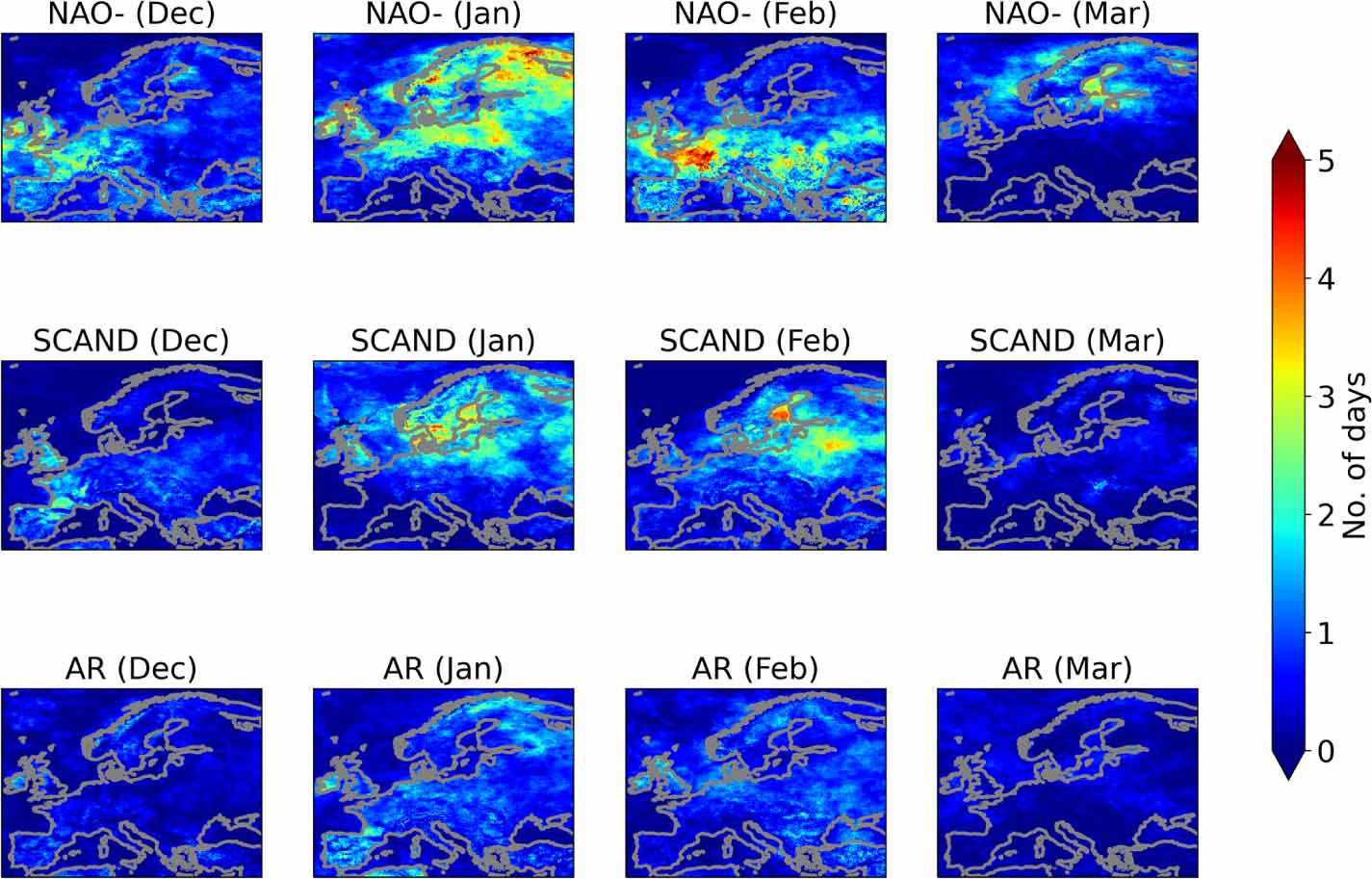
Overall, figure 4 supports what previous studies have found: (a) that large-scale circulation patterns influence the energy demand [22, 30, 31] and the wind power generation over Europe [22, 32, 33, 43], and (b) that blocking patterns are associated with anomalous cold and low-wind speed conditions over Northern and Central Europe, which, in turn, increase the demand and reduce the wind power generation [22, 30, 33, 43–45].