Reanalysis-based contextualization of real-time snow cover monitoring from space

Simon Gascoin; Diego Monteiro; Samuel Morin

doi:10.1088/1748-9326/ac9e6a

1. Introduction

Various stakeholders including citizens seek real-time information on the current state of the environment (Hewitt et al 2012, Vaughan and Dessai 2014). The availability of real-time meteorological data, accompanied by their climatic context contributes to increasing environmental awareness and provides relevant information for the real-time management of challenging situations (Overpeck et al 2011). Social media now allows a swift dissemination of such information reducing barriers between scientific organizations and society (Pearce et al 2019).

In situ meteorological observations are critically relevant but they often provide sparse sampling of hydrometeorological variables, especially in mountain regions (Hik and Williamson 2019). Satellites provide real-time, spatially continuous data on some essential climate variables (Bojinski et al 2014). However, satellite observation time periods are often too short to characterize climatological references, especially at the local scale. On the other hand, meteorological reanalyzes provide information over longer time scales but are often not available in real-time. For example, the global Modern-Era Retrospective analysis for Research and Applications (MERRA-2) is published with a latency of a few weeks (Reichle et al 2017). ERA5 is updated with a shorter latency of 5 d. However, the fully quality-checked final product is released two months later (Hersbach et al 2020). In addition, the MERRA-2 and ERA5 spatial resolutions are approximately 50 km and 30 km respectively, which is too coarse for some applications. More advanced reanalyzes are updated with longer latency. For example, ERA5-Land (approximately 9 km resolution) is available with a 2–3 month delay (Muñoz-Sabater et al 2021), which makes it unsuitable for real-time applications.

Hence, there is often a gap between the availability of real-time products and long-term records at the climactic time scale due to the lack of immediate real time availability. Many environmental variables are related to these time scales, making this situation unfortunate; however, the combination of various sources of information can be used to bridge this gap and build upon their benefits across temporal and spatial scales (AghaKouchak and Nakhjiri 2012, Notarnicola 2022).

Here, we exemplify such an approach, focusing on the development of real-time monitoring of the snow cover area based on the combination of satellite and reanalysis data. The current well-established methods used to retrieve the snow cover extent from spaceborne sensors have been developed since the 1980s. In particular, the Moderate-Resolution Imaging Spectroradiometer (MODIS) multispectral optical sensor onboard Terra has enabled the daily measurement of the snow cover area at 500 m resolution since 2000 (cloud-permitting). MODIS snow products are distributed by the National Snow and Ice Data Center (NSIDC) to alleviate the processing of the MODIS data by end users. These products indicate the presence of snow along with a cloud mask (Hall and Riggs 2015).

Based on MODIS data only, the first author has developed a web-based tool to analyze in real-time the snow cover area in the Alps (Alps Snow Monitor n.d.). This tool has attracted some attention, especially in the context of the severe drought that affected the Alps during the winter of 2022 (European Commission. Joint Research Centre 2022). For example, this tool allowed us to reveal that on 2 March 2022, the snow cover area in the Alps had reached its lowest value since 2001. This finding was published on 5 March 2022 (Gascoin 2022). Later, we showed that the 2022 snow cover area in the Alps reached its minimum earlier than any other year since 2001 (figure 1).

Figure 1. Refer to the following caption and surrounding text. — **Figure 1.** Tweets published on 5 March 2022 and 10 June 2022 to communicate on the current status of snow cover in the Alps.
Download figure:
Standard image High-resolution image

Other similar tools use the MODIS record to provide information to the general public, e.g. 'SnowCloudMetrics' (Crumley et al 2020) or 'Snow Today' (Snow Today Article | NSIDC Reports n.d.). However, although the MODIS data record already spans 22 years, it does not reach the 30 year standards that are used by meteorological agencies to define climatological references. Hence, it could lead to non-robust assessments of the true extend of a given situation. Given the interest in having real-time information regarding snow cover in the Alps, we sought to provide a more robust contextualization of the MODIS observations. To this end, we used longer reanalysis data spanning the entire European Alps domain at a sufficiently fine spatial resolution for this mountain environment, namely, the Uncertainties in Ensembles of Regional ReAnalysis (UERRA) reanalysis at 5.5 km resolution (Soci et al 2016, Morin et al 2021). A 30 year-long snow cover area climatology was generated from this dataset using machine learning to de facto generate MODIS-like data using the reanalysis for the time period before the onset of the MODIS observations. Here, we describe the tool and the method for generating this contextualization dataset. We discuss the implications of bringing together the best of the two worlds of space-borne observations (real-time, short time periods) with reanalysis data (longer-term).

2. Method

2.1. Remote sensing data

Our application was designed to map and plot the evolution of the snow-covered area over a large region (>10⁴ km²), such as the entire Alps range or one of its main river catchments (figure 2). At this scale, the Terra/MODIS MOD10A1 snow products offer the best compromise in terms of accuracy, spatial resolution, revisit and duration (Dietz et al 2012, Dumont and Gascoin 2016).

Figure 2. Refer to the following caption and surrounding text. — **Figure 2.** Map of the five regions of interest used to compute the snow cover area.
Download figure:
Standard image High-resolution image

From the MOD10A1 snow product, we extracted the NDSI_Snow_Cover field. This field indicates the normalized difference snow index (NDSI) for snow-covered pixels. The NDSI is computed using the green and shortwave infrared bands and is used to identify snow, based on its higher reflectance in the visible portion of the spectrum compared to the shortwave infrared (Hall et al 2002). Approximately 50% of the pixels were flagged as clouds; therefore, we implemented a gap-filling algorithm using linear interpolation in the time dimension and on a pixel basis. This algorithm was limited to fill a maximum of 10 d, which is usually sufficient to fill approximately 90% of the cloud pixels in temperate regions (Gascoin et al 2015). Although more sophisticated algorithms exist to fill the gaps in MODIS snow cover products, linear interpolation in the time dimension is an acceptable trade-off between efficiency and accuracy and sufficient for our scale of analysis (Parajka and Blöschl 2008, Gascoin et al 2015). The linear interpolation was bounded to a time window of 5 d to limit the computation time. The resulting series of daily gap-free NDSI was converted to a series of binary snow cover maps (snow/no-snow) using the threshold NDSI > 0.2. This threshold corresponds to a snow cover fraction of approximately 30% following the relationship which was used in the previous MOD10A1 products (Salomonson and Appel 2004). This threshold is arbitrary but necessary as a binarization of the snow cover fraction must be done to allow for the computation of a snow cover duration map. Then, daily gap-filled snow cover maps over 2000–2021 were aggregated to a 5 km resolution by majority resampling. The snow-covered fraction of a given region was computed from this time series of 5 km resolution snow maps and subsequently used as training data for the machine learning algorithm described below.

2.2. Reanalysis data

We used the UERRA 5.5 km reanalysis data, which covers all of Europe and is available from 1961 to 2015 (Soci et al 2016, Lopez 2019, Morin et al 2021). This reanalysis uses the ERA-40 (from 1961 to 2002) and ERA-Interim (from 2002 to 2015) global reanalyzes as input to the regional numerical weather prediction system HARMONIE (Bengtsson et al 2017) at 11 km resolution, downscaled to 5.5 km resolution. These predictions were combined with an analysis system enabling correction of the raw predictions of HARMONIE using in situ observations of temperature, relative humidity and precipitation (Bazile et al 2017). During a second step, the reanalysis of near-surface atmospheric variables at 5.5 km resolution was used to drive the snow cover model Interactions between Soil, Biosphere and Atmosphere-Explicit Snow (ISBA-ES) as part of the SURFEX modeling platform (Masson et al 2013). ISBA-ES snow cover model is an intermediate complexity 12 layers snow scheme (Boone and Etchevers 2001, Decharme et al 2016). This reanalysis provides estimates of daily snow depth values at 5.5 km resolution (Bazile et al 2017). The full documentation is available along the UERRA dataset in the Copernicus Climate Data Store (Lopez 2019). The UERRA snow depth data available from 1961 to 2015, were used as a predictor for the machine learning approach described below.

2.3. Model

We trained a statistical model to predict the snow cover area of a given region of interest at the daily time step. For a given day, the input samples (predictors) are the snow depth values on that day extracted over the region of interest from the UERRA reanalysis. We tried linear regression and gradient boosting, two commonly used machine learning algorithms in geosciences and ecology. Gradient boosting is a flexible and efficient nonparametric statistical learning technique for classification and regression (Friedman 2001). We used the implementation of the linear regression and gradient boosting regression functions in the Scikit-learn Python module (Pedregosa et al 2011). The model was optimized by minimizing the squared error between the training and predicted data. The data were randomly split into training (75%) and test (25%) subsets. For the gradient boosting, we set the learning rate to 0.1 (default value), the number of boosting stages to 100 (default value) and did not activate stochastic subsampling. The function to measure the quality of a split was kept to the default Friedman mean squared error.

We fit a different model for each region of interest using the same workflow. We considered five regions of interest: (a) the entire Alps range and the intersections of the Alps range polygon with the river basins of the Rhine, Rhône, Danube and Po. The Alps and the river basin polygons were sourced from the European Environmental Agency.

Indeed, we chose to divide the Alps domain into river basins to characterize the spatial variability of the snow cover within the Alps range and to strengthen the link with external water resource monitoring tools in a more meaningful way than an aggregation at the scale of the entire Alps domain.

We used the region-calibrated model to predict the snow-covered fraction of each region from 1991 to 2018. This series was completed with the MODIS data to generate a 30 year climatology until 2021. We considered that a snow season starts on 1 November and ends on 1 July. Although the seasonal snow cover can last beyond July in the Alps, we restricted our analysis to the core of the snow season to reduce computational cost. In addition, our method is not adapted to detect patchy snow cover, which is predominant during late summer. The predicted snow cover time series were then aggregated by day of year in the form of percentile values corresponding to 0 (minimum), 25 (first quartile), 50 (median), 75 (third quartile) and 100 (maximum). These daily statistics formed the climatology that was used below. The climatology was uploaded as a public asset to the Earth Engine server.

2.4. Real-time implementation

The real-time application was implemented in Google Earth Engine (Gorelick et al 2017). MOD10A1 products are quickly ingested in Earth Engine so that the latency between sensing time and the availability of the images is usually below 4 d (see appendix).

The user must select a region of interest (Alps, Rhine, Po, Rhône or Danube). Then, the application computes the snow cover area from the beginning of the snow season until the latest available MODIS snow product using the same method as described above, i.e. after linear interpolation of the cloud pixels. The resulting series is concatenated to the climatology and transferred from the server to the client, i.e. any web browser that calls the application. The application returns the data as an interactive chart, which displays the plotted values if the user hovers the mouse on the lines. If the user enlarges the chart, the plotted data can be exported as comma separated values for further analyses. The computation was split into two periods from 1 November to 31 December and from 1 January to 1 July to avoid hitting current Earth Engine usage limits for noncommercial users. The charts were embedded in a webpage of the Séries Temporelles blog (Alps Snow Monitor n.d.) but can be run in a separate window of a web browser.

3. Results

3.1. Evaluation of the model

Figure 3 shows the performance of the gradient boosting regressor that was used to predict the snow-covered fraction of the Alps from UERRA data. The predicted samples were not used in the model optimization. The model performance is high, with R² = 0.98 and a root mean squared deviation (RMSD) value of 4%. A linear regression model was also tested but performed poorly, with an R² value of −1.41 and RMSD value of 39%. Figure 4 compares the output of the linear regression against the gradient boosting regression for the first year of the training dataset as an example, showing the large noise level in the linear regression model.

Figure 3. Refer to the following caption and surrounding text. — **Figure 3.** Evaluation of the predicted snow cover fraction with the gradient boosting regression using the test samples (the entire domain of the Alps).
Download figure:
Standard image High-resolution image

Figure 4. Refer to the following caption and surrounding text. — **Figure 4.** Comparison of the linear (left) and gradient boosting (right) regression methods to predict the snow cover fraction during the snow season 2000–2001 over the entire Alps region.
Download figure:
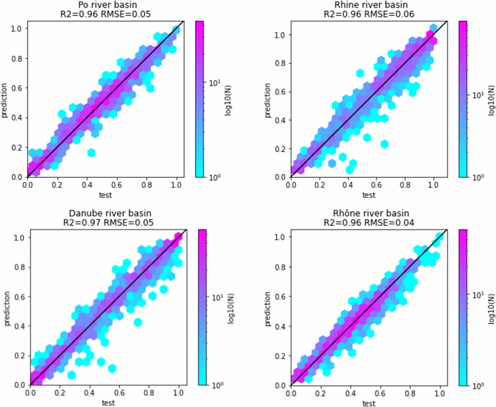
Standard image High-resolution image

We also obtained an accurate model for every river basin subregion (figure 5). The performances were slightly lower, with R² values ranging from 0.96 to 0.97 and RMSD values ranging from 4% to 6%. Figure 6 shows an example of the predicted snow cover fraction during two snow seasons 2004–2006 for the Rhône subregion.

Figure 5. Refer to the following caption and surrounding text. — **Figure 5.** Evaluation of the predicted snow cover fraction using the test samples for every subregion.
Download figure:
Standard image High-resolution image

Figure 6. Refer to the following caption and surrounding text. — **Figure 6.** Observed and predicted snow cover fraction over the Rhône region during two consecutive snow seasons (2004–2005, left, and 2005–2006, right).
Download figure:
Standard image High-resolution image

3.2. Output of the application

Figure 7 shows a screenshot of the application as of 31 July 2022 when the Po subregion was selected. Figure 8 compares the output of the application before and after the introduction of the 30 year climatology. In the former version, 20 years of MODIS data were used to provide a range of variability. In the new version, we plot the current year over the percentiles from the 30 year climatology (1991–2020). This new version reveals the exceptional trajectory of the snow cover area in the Alps during the hydrological year 2021–2022, as it remained well below the median during almost the entire melt season and eventually dropped below the 30 year minimum in June. The new application also indicates that the snow deficit was even more severe in the Po river basin since the snow cover fraction remained below the 30 year minimum during most of the snow melt season in 2022 (figure 7).

Figure 7. Refer to the following caption and surrounding text. — **Figure 7.** Screenshot of the application (here the Po river basin subregion was selected). The red line shows the daily snow cover area of the current hydrological year, whereas the blue line shows the daily median snow cover area from the 30 year climatology (1991–2020).
Download figure:
Standard image High-resolution image

Figure 8. Refer to the following caption and surrounding text. — **Figure 8.** Alps snow monitor application before (left) and after (right) the upgrade including the 30 year climatology. Note that the new application was upgraded to start on 1 October, whereas the previous version only started on 1 November, which explains why the red curves do not look similar, but they are identical over the common period (1 October–1 July).
Download figure:
Standard image High-resolution image

4. Discussion and conclusion

Cloud computing platforms enable the development of services based on remote sensing data streams without having to develop infrastructure (data storage, updating, cataloging, processing, publishing). We developed our application in the Google Earth Engine, but it could be implemented in another server since it uses only public data and standard remote sensing image processing algorithms that are implemented in open-source software.

We find that the error of our statistical model data slightly increased from the entire Alps domain to the river basin subdomains. These minimal performance losses were expected due to the reduction of the domain size, which tends to increase the uncertainty in MODIS data. It also reflects the effect of the uncertainties in the UERRA reanalysis at the local scale. This suggests that further reductions in the domain size could lead to increased errors, limiting the relevance of this approach for local-scale real-time snow cover monitoring. Our model was trained after applying a NDSI threshold of 0.2 to capture lower snow fractions than the standard 0.4 threshold, however it may fail to retrieve areas with less than 30% of snow cover (Salomonson and Appel 2004). The gradient boosting should be trained again if this threshold is changed to capture lower snow fractions. We provide the source code of the entire pipeline to do this (see Data and code availability below). The integration of higher resolution remote sensing products is a solution to focus on more local scales (e.g. ski resorts, national parks, etc.). Methods exist that allow downscaling MODIS to 20 m resolution in real time using Sentinel-2 products (Revuelto et al 2021). Predictions into the future are the next step to this approach, which could be feasible using numerical weather prediction output instead of reanalysis data (Andersson et al 2021).

Another key limitation of this application is that it does not provide information on the snow water equivalent or streamflow. Both variables would be more directly useful for water management. In snow-dominated catchments, streamflow can be simulated in real time using MODIS data and the Snowmelt Runoff Model (Rango and Martinec 1979, Sproles et al 2016). This could be done with the same platform if stream gauge data are available to calibrate the model parameters. Mapping the distribution of the snow water equivalent might be more challenging, especially in mountain catchments, and requires a more advanced combination of model and remote sensing data (Dozier et al 2016).

Despite these limitations, the current application is relevant to characterize the snow cover and indirectly the status of the Alps water resources in real time. This is especially relevant during periods of extreme weather, such as the 2022 snow drought. It allows everyone to figure how extreme the current condition is, thereby contributing to a better understanding of the climate system and its evolution.

Given the increasing availability of remote sensing products and land surface reanalysis, a similar approach could be implemented to characterize the evolution of other key variables such as soil moisture, surface water area, evapotranspiration, vegetation phenology, etc.

Acknowledgments

This work was supported by the ANR TOP project, Grant No. ANR-20-CE32-0002 of the French Agence Nationale de la Recherche.

Data and code availability

A pre-release of the application and its previous version are available at https://labo.obs-mip.fr/multitemp/apps/alps-snow-monitor/. The data and Python code to train the model and infer the snow cover fraction climatology is publicly available on GitHub (https://github.com/sgascoin/ModisExtension/releases/tag/v1). Earth Engine JavaScript code to compute the snow cover fraction from MODIS products and the code of the web application are publicly available in this git repository (https://earthengine.googlesource.com/users/sgascoin/apps). We acknowledge Dongdong Kong (China University of Geosciences) for sharing the temporal interpolation code (https://github.com/gee-hydro/gee_docs).

Data availability statement

The data that support the findings of this study are openly available at the following URL: https://github.com/sgascoin/ModisExtension.

: Appendix

Latency of MOD10A1 snow products in Google Earth Engine

We define latency as the difference between the acquisition time of the raw data by the MODIS sensor and the ingestion time in Earth Engine. This latency includes the time to generate and distribute the products from the raw MODIS observations by the NASA National Snow and Ice Data Center Distributed Active Archive Center (NSIDC DAAC).

In Earth Engine, MODIS image collections contain a list of daily global mosaics. The 'version' field in the properties of each mosaic (i.e. image) in the ingestion epoch in microseconds. However, each mosaic's granules were obtained at different times within the time range that the mosaic covers (24 h). Since this information is not preserved in Earth Engine, we approximate the acquisition time of a MODIS image as the mean of the end and start time properties of the image.

We computed latency times for all MOD10A1 images acquired in 2021 that are available in Earth Engine (figure A1). We found that the images were available with a median time of 2.34 d, and 90% of the images were available with a latency of 4.36 d. For the current set of images acquired in 2022 (on 3 July 2022), the median latency was 3.39 and 90th percentile was 9.07 d. In 2017 and 2018, Earth Engine engineers reported authentication problems with NSIDC downloads which significantly delayed the availability of MOD10A1 products, but this did not happen again in the recent years.

Figure A1. Refer to the following caption and surrounding text. — **Figure A1.** Histogram of latency times of MOD10A1 products available in Earth Engine. Latency values were computed from all products acquired in 2021 (365 images).
Download figure:
Standard image High-resolution image

Dates

Peer review information