

Abstract
The ocean mixed layer temperature equation is used to estimate the surface net heat flux from drifter measurements. The net heat flux is determined for both the climatologic and tropical cyclone (TC) conditions. The spatial distributions of the drifter-derived heat fluxes under both the two conditions are similar to those derived from satellite observations. However, the drifter-derived climatologic heat flux appears to be weaker in magnitude than that derived from satellites, and performs better in closing the energy budget with a global mean value of 3.9 W m−2. The drifter-derived heat flux also performs better than the satellite-derived heat flux under TCs, using the buoy observations as a reference considering metrics such as the meen error, mean absolute error, root mean-square error and percent bias. The spatially averaged mean net heat flux derived from drifters under TCs is −124 W m−2 at 10° N, and decreases to −85 W m−2 at 30° N, however, these values are much larger than those obtained from satellites (−63 W m−2 and −21 W m−2, respectively). As additional components for the mixed layer temperature equation, both the entrainment velocity and eddy diffusivity in climatology show large amplitudes in regions with strong currents such as the Western Boundary Current and Antarctic Circumpolar Current. However, under TC conditions large values of the entrainment velocity and eddy diffusivity mostly appear in regions with strong winds.
Export citation and abstract BibTeX RIS

Original content from this work may be used under the terms of the Creative Commons Attribution 4.0 license. Any further distribution of this work must maintain attribution to the author(s) and the title of the work, journal citation and DOI.
1. Introduction
The net air-sea heat flux (Qnet), the sum of the net downward shortwave radiation (SW), the net upward longwave radiation (LW), the latent heat (LH) and sensible heat (SH) fluxes, affects the temperature structure of the upper ocean and in the atmospheric boundary layer (Frankignoul and Reynolds 1983, Cayan 1992, Delworth 1996, Halliwell 1998, Alexander et al 2000, Seager et al 2000, Dong and Kelly 2004, Foltz et al 2013). Therefore, Qnet is a key component in Earth system models (Semtner and Chervin 1992, Stockdale et al 1993) and is of great importance for understanding global climate and climate change. In addition, Qnet is closely related to the weather variability on both regional and global scales. For example, many studies have shown that Qnet is of considerable importance for the prediction of tropical cyclone (TC) tracks and intensity (Schade and Emanuel 1999, D'Asaro et al 2007). Consequently, high quality Qnet products are needed for the characterization, attribution, and modeling of weather, climate, and ocean variability (Curry et al 2004, Fairall et al 2010, Gulev et al 2010).
Although considerable effort has been expended in improving the quantification of radiative and turbulent heat transfer at the sea surface through better measurements and improved modeling, the representation of surface heat exchange processes and the net heat flux, Qnet, are still not accurately determined (Dong et al 2007, Song and Yu 2013, 2017, Song 2020). Uncertainties in estimating Qnet on regional to global scales arise primarily from uncertainty in the surface variables in the air‐sea boundary layers and the empirical bulk flux parameterizations (Weare 1989, Gleckler and Weare 1997, Josey 2001, Brunke et al 2011, Yu et al 2013, Weller et al 2016, Yu 2019). The globally averaged mean Qnet, which is an important parameter for the evaluation of heat flux products, represents a mean over the global ice-free open ocean. The average of the long-term mean Qnet should be closed to within 2–3 W m−2 but not to exactly zero (Serreze et al 2007, Bengtsson et al 2013). However, the available flux products have not yet reached an accuracy to achieve such a balance (Josey et al 2013, Yu et al 2013), whereas most products are warm-biased so that they cause excessive heating of the ocean at a rate of between 0 and 30 W m−2 (Song and Yu 2013, Song 2020). Further, the precise magnitude of the extreme heat fluxes at the synoptic scale during TCs can provide another important benchmark for the assessment of the various heat flux products. Under TC conditions, the most striking feature is the dramatic reduction in Qnet, with an extreme decrease during an individual TC case reaching as much as approximately 800 W m−2 (Song et al 2021). While all four components of Qnet contribute to its reduction during TCs, the dominant contribution is from the decreased SW radiation, with the increased LH, the decreased LW radiation and the enhanced SH providing decreasing contributions (Song et al 2021). Consequently, better estimates of Qnet are desired both at the global climate scale and for local extreme weather event.
Based on ocean mixed layer dynamics, variations in mixed layer temperature are governed through the heat balance in the surface mixed layer, which is driven by the surface air-sea heat exchanges, horizontal advective and diffusive processes in the mixed layer, and entrainment processes at the base of the mixed layer (Dong et al 2007). Because the huge amounts of surface drifters can accurately measure the mixed layer temperature and current velocity, even under the most destructive TC conditions, they may provide alternative estimates of heat exchange across the air-sea interface. In the present paper, the close relationship between the mixed layer temperature and air-sea heat fluxes is used to estimate Qnet from the large collection of surface drifters. The assessment of Qnet for both the global climatology and under TC conditions are addressed, separately.
2. Data and method
2.1. Drifter data
The surface satellite-tracked drifter dataset (Lumpkin and Centurioni 2019) covering the period 1988–2013 is used to estimate terms in the mixed layer temperature equation for the global ocean. The dataset consists of latitude and longitude arrays of mixed layer temperature and current velocity components with 6-hourly temporal resolution, obtained by the procedure of optimum interpolation. During the period 1988–2013, over 17 000 drifters have been deployed globally (figure S1), and more than 24.7 million individual measurements are available (figure S2). These drifters have submerged 'holy sock' drogues centered at a depth of 15 m to reduce the large biases induced by processes at air-sea interface (e.g. winds and breaking waves) and thereby accurately measure mixed layer temperature and current velocity, even under the most intense TCs. Therefore, these globally distributed drifters allow for the possibility of accurately estimating the heat exchange across the air-sea interface from the mixed layer temperature equation.
2.2. Mixed layer depth (MLD) data
The thickness of the mixed layer is a key factor for determination of the mixed layer temperature. The MLD used in the present study are determined by a temperature criterion from the Simple Ocean Data Assimilation version 3.3.1 monthly mean ocean reanalysis dataset, with a spatial resolution of 0.5° × 0.5° spanning from 1988 to 2013.
2.3. Satellite-derived air-sea net heat flux data
Satellite-derived net heat flux data with daily temporal resolution obtained from the Japanese Ocean Flux Data Sets with Use of Remote Sensing Observations (J-OFURO) research project based on observational information obtained from various earth observing satellites is used to compare with the drifter-derived heat flux. In the present study, the third-generation dataset, J-OFURO3, is adopted. The satellite data, which comes with a horizontal resolution of 0.25° × 0.25°, is interpolated onto a 0.5° × 0.5° grid to be consistent with the MLD data during 1988–2013.
2.4. TC data
Observations of TC occurrence during 1988–2013 were acquired from the best track data provided by the Joint Typhoon Warning Center for the Western Pacific Ocean, the Indian Ocean, and the Southern Hemisphere, and the National Hurricane Center and Central Pacific Hurricane Center for the Atlantic and Northeast and Central Pacific Oceans. This TC track data is produced with 6-hourly temporal resolution.
2.5. Buoy-derived air-sea net heat flux data
Buoy-derived net heat flux data with daily temporal resolution obtained from the Global Tropical Moored Buoy Array (GTMBA) and Ocean Climate Stations (OCSs) is used to compare with the drifter-derived and satellite-derived heat fluxes. In the present analysis, 36 buoys located in the global tropical oceans from the GTMBA are used in climatology, and 8 buoys from the GTMBA and 1 buoy from the OCS are applied under TC conditions.
2.6. Method
In order to obtain the heat flux across the air-sea interface, we solve the mixed layer temperature equation (Dong et al 2007), which can be expressed as:
where T is the mixed layer temperature, v is the mixed layer current velocity including both the zonal and meridional components, ρ (1027 kg m−3) is the reference density of seawater, cp (4000 J kg−1 K−1) is the specific heat of seawater at constant pressure, h is the MLD, and ΔT is the temperature difference across the bottom of the mixed layer (set to be 0.5 °C). Here Q is the sum of the surface net heat flux that is positive into the ocean and the downward radiative heat flux at the bottom of the mixed layer, we is the entrainment velocity, and k is the eddy diffusivity.
Equation (1) is a nonhomogeneous linear equation, where Q, we and k are considered as unknown variables, with  ,
,  and
and  being the corresponding coefficients. The three coefficients on the left-hand side and temperature tendency and horizontal advection terms on the right-hand side can be determined from the drifter measurements, MLD data and coefficient constants mentioned above. To estimate Q, we and k by solving equation (1), the major steps are as follows:
Step 1, estimate partial derivatives of  using the central difference method based on each set of five consecutive drifter measurements along a trajectory (figure S3).
Step 2, estimate Q, we and k at the central location (location 4 in figure S3) by solving the following three equations derived from equation (1) with three sets of the above partial derivative estimates. Note we suppose Q, we and k remain unchanged during the observed period of 1.5 day
Step 3, repeat the above processes along each drifter trajectory. Estimated Q, we and k from all drifters are further grouped into bins of 0.5° × 0.5°globally. Here the 0.5° × 0.5° bins are adopted to be consistent with the spatial resolution of the MLD.
Step 4, the same as described in step 3 but under TC conditions. The estimated Q, we and k under TCs are grouped into bins of 5° × 2.5° globally. Because the average size of a TC is around 500 km in diameter, 5° in zonal direction is used. Half of this distance is applied in the meridional direction due to less coherence of ocean variability. Specifically, we also grouped these estimated Q, we and k in the along-track and cross-track coordinate system under TCs.
3. Results
3.1. Global long-term mean net heat flux
Global distributions of the climatological entrainment velocity, eddy diffusivity and net heat flux during the study period (1988–2013) are obtained. To reduce the noise from mesoscale features and focus on its larger-scale pattern, these climatologic values are smoothed in space using a mean filter with the smoothing lengths of 1° in latitude and 2° in longitude.
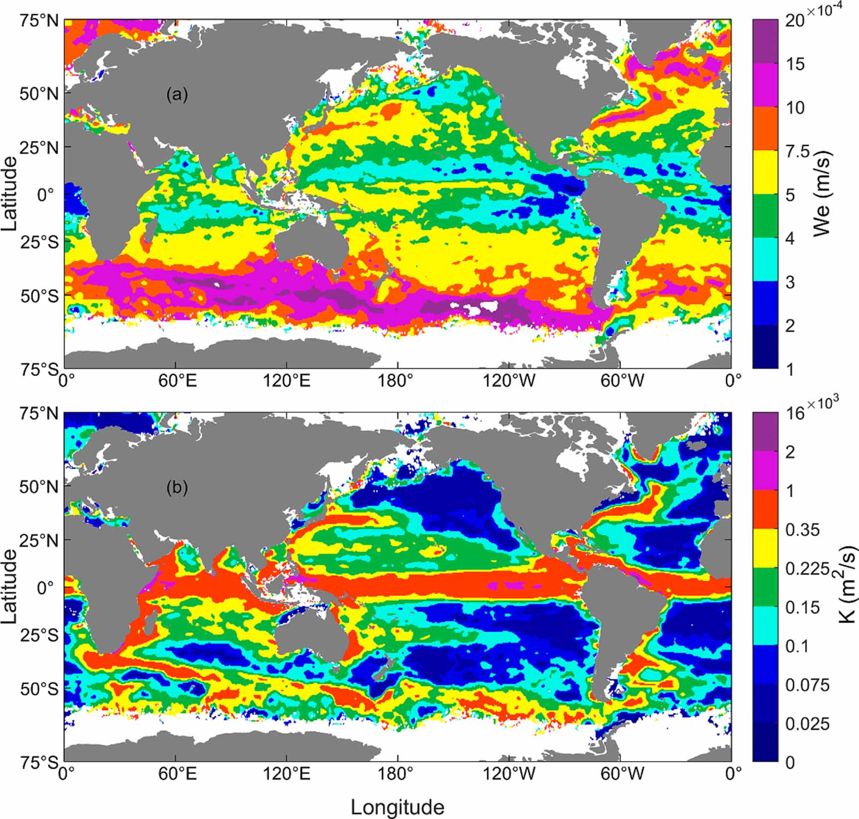
Large values of the entrainment velocity appear in regions of strong currents such as near the Kuroshio Current, the Gulf Stream, and the Antarctic Circumpolar Current (ACC) (figure 1(a)). High rates of mixed layer deepening may contribute to the strong entrainment in the Western Boundary Current (WBC) regions, such as the Kuroshio Current (Qu 2003), while the strong prevailing westerlies and the associated intense upwelling may contribute to the strong entrainment in the ACC regions. On average, the long-term mean entrainment velocity is about 6.2 × 10⁻⁴m s−1 on a global scale, which is on the same order of magnitude as that found by Nagai et al (2005). High values of the eddy diffusivity appear in the western boundaries around the global ocean, the ACC region, as well as along the global equatorial belts (figure 1(b)). These large values are likely to correspond with the generation of mesoscale eddies, baroclinic instability, and tropical instability waves, respectively (Zhurbas and Oh 2004, Zhurbas et al 2014). In general, the spatial pattern of the eddy diffusivity bears much resemblance to that obtained by Zhurbas et al (2014). The global distributions of both the entrainment velocity and eddy diffusivity verify that the mixed layer temperature equation has the potential to estimate the surface net heat flux accurately from the drifter dataset.

Figure 1. Spatial distributions of the (a) entrainment velocity at the base of the mixed layer, and (b) eddy diffusivity in the mixed layer based on drifter measurements from 1988 to 2013.
Download figure:
Standard image High-resolution imageThe drifter-derived net heat flux in climatology is shown in figure 2(a). The ocean gains heat primarily in the tropics, especially in the equatorial cold tongue regions, and releases heat primarily at high latitudes especially in the significant WBC systems such as the Kuroshio Current and Gulf Stream in the Northern Hemisphere and the Agulhas Current in the Southern Hemisphere. The high-latitude North Atlantic Ocean appears to be another region of significant heat transfer into the atmosphere from the underlying ocean, which is likely related to the deep-water formation there where heat is released to make surface water dense enough to sink. In addition, heat absorption into the ocean also occurs in the four major eastern boundary upwelling regions; namely the California and Peru-Chile upwelling regions in the Pacific Ocean, the Canary and Benguela upwelling regions in the Atlantic Ocean, and the Somali current upwelling region on the western boundary of the Indian Ocean. The upwelling in these regions results in low sea surface temperatures (SSTs) that lead to stronger heat absorption from the atmosphere.

Figure 2. Spatial distributions of the (a) drifter-derived net heat flux, (b) satellite-derived net heat flux from the J-OFURO3 flux product, and (c) difference between the two net heat fluxes (drifter-derived minus satellite-derived). Positive values in (a) and (b) suggest that the heat transfer is into the ocean in climatology during 1998–2013.
Download figure:
Standard image High-resolution imageTo see whether the spatial pattern of the drifter-derived heat flux is similar with that of the satellite-derived heat flux, figure 2 shows the globally distributed Qnet derived from drifters (figure 2(a)) and from satellites using the J-OFURO3 flux product (figure 2(b)). The spatial structure of the drifter-derived heat flux bears considerable resemblance to the satellite-derived heat flux and has a high spatial correlation coefficient of 0.83, which is statistically significant at the 99% confidence level. However, the drifter-derived heat flux is much smaller in magnitude than the satellite-derived heat flux over nearly the entire global oceans, especially for the EC and WBC regions (figure 2(c)). Quantitatively, the drifter-derived heat fluxes have a global mean positive value of 16.8 W m−2 and negative value of −14.4 W m−2, while the associated satellite-derived values are 36.3 W m−2 and −28.7 W m−2, respectively. Consistently, the spatially averaged drifter-derived heat flux in the regions of Kuroshio Current, Gulf Stream, Agulhas Current, Equatorial Current and ACC are −13.8, −25.3, −7.0, 18.2, and 5.7 W m−2, respectively, all of which are weaker than the corresponding satellite observations of −23.7, −43.3, −18.3, 48.3 and 16.8 W m−2. In addition, both the two heat flux estimates show similar seasonal variations with heat released to the atmosphere in each hemisphere's winter and transferred into the ocean in each hemisphere's summer at all latitudes, but with different magnitudes.
To further compare the global heat budget balance (Isemer et al 1989, Josey et al 1999, Schuckmann et al 2016, Liu et al 2017, Valdivieso et al 2017) between the drifter-derived and satellite-derived heat fluxes, the global mean Qnet is calculated based on the following area-weighted average equation:
Results show that the globally averaged long-term mean of Qnet for the drifter-derived and satellite-derived heat fluxes (averaged in areas where there are no missing data for either of the two fluxes) are 3.9 W m−2 and 23.5 W m−2, respectively. Obviously, the drifter-derived heat flux is closer to the physical constraint on the global mean Qnet of 2–3 W m−2 (Serreze et al 2007, Bengtsson et al 2013), which shows its better performance in closing the heat budget at the ocean surface.
3.2. Net heat flux under TC conditions
Because in situ observations are difficult and rare during the passage of a TC, the composite of Qnet is computed by using drifter observations within 7Rmax of TC tracks in the TC-coordinate system. The left-hand panels of figures 3(a)–(c) show the composite Qnet estimates computed for all TCs, tropical storms (TSs) and category 1–5 TCs, respectively. These TC related air-sea heat fluxes all have an obvious strong left-to-right asymmetry with the maximum values located on the right side of TC tracks. Such left-to-right asymmetry primarily arises from the asymmetric distributions of TC wind structure, with the strongest wind stress occurring on the right side in the Northern Hemisphere and left side in the Southern Hemisphere of TC tracks (Price 1981), respectively. It should be noted that in this analysis, the left-to-right asymmetric spatial pattern in the Southern Hemisphere has been adjusted to be consistent with that in the Northern Hemisphere. Specifically, the maximum heat release increases from 80 W m−2 to 175 W m−2 as TCs intensify from TSs to category 1–5 TCs. Detailed comparisons of the drifter-derived net heat fluxes under various intensity TCs are listed in table 1.

Figure 3. The drifter-derived (a)–(c) net heat flux, (d)–(f) entrainment velocity, and (g)–(i) eddy diffusivity under (a), (d), (g) all TCs, (b), (e), (h) TSs, and (c), (f), (i) category 1–5 TCs. Note that the left-to-right asymmetric spatial pattern in the Southern Hemisphere has been adjusted to be consistent with that in the Northern Hemisphere.
Download figure:
Standard image High-resolution imageTable 1. Comparisons of the maximum and averaged values of the drifter-derived net heat flux Q, entrainment velocity we, and eddy diffusivity k under all TCs, TSs, and category 1–5 TCs, respectively.
| Terms | All TCs | TSs | Category 1–5 TCs | |||
|---|---|---|---|---|---|---|
| Max. | Ave. | Max. | Ave. | Max. | Ave. | |
| Q (W m−2) | −115 | −74 | −80 | −40 | −175 | −140 |
| we (m s−1) | 8.5 × 10⁻⁴ | 6.5 × 10⁻⁴ | 7.4 × 10⁻⁴ | 5.9 × 10⁻⁴ | 13 × 10−4 | 8.6 × 10⁻⁴ |
| k (m2 s−1) | 717 | 475 | 646 | 441 | 1039 | 593 |
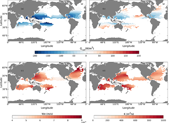
Further, we extend the extreme air-sea heat fluxes occurring under TC conditions to the main TC basins. Figure 4(a) shows the spatial distribution of the drifter-derived heat fluxes resulting from the passage of TCs. In general, heat is released from the underlying ocean surface with the magnitudes decreasing poleward, which may be correlated with the spatial distribution of the SSTs that almost decrease linearly with the increasing latitude. The satellite-derived heat flux shows a similar spatial pattern but with smaller magnitudes (figure 4(b)), and there are regions in midlatitudes of both the two hemispheres where heat is even released from the atmosphere to the ocean. Specifically, the spatially averaged mean Qnet are −186, −124, −112, and −85 W m−2 at 5° N, 10° N, 20° N, and 30° N, respectively, all of which are larger in magnitude than the corresponding satellite-derived results of −89, −63, −29, and −21 W m−2. This suggests that the drifter-derived heat flux estimates as a result of the passage of TCs is 2–4 times those derived from satellite data. Because satellite measurements are strongly biased by drop-outs from cloud coverage, the accuracy of the satellite-derived heat flux under TCs may be seriously degraded. However, the drifter measurements are of high accuracy, with the use of drogues centered at a depth of 15 m to reduce the large bias induced by wave processes at the air-sea interface and the Global Position System in localization, even under TCs. Therefore, the drifter-derived heat fluxes should be more realistic than the satellite-derived heat fluxes under TC conditions.
Figure 4. The drifter-derived (a) net heat flux, (c) entrainment velocity and (d) eddy diffusivity based on the mixed layer temperature equation, and (b) the satellite-derived net heat flux from the J-OFURO3 flux product. All are under TC conditions.
Download figure:
Standard image High-resolution image
Furthermore, taking the heat flux obtained from 8 buoys of the GTMBA and 1 buoy of the OCS as a subset for evaluation, we further compare the drifter-derived and satellite-derived heat fluxes under TCs. As shown in figure S4, the errors of the drifter-derived heat flux are much smaller compared with those of the satellite-derived heat flux, with the mean errors being 12.3 and 128.9 W m−2, respectively. Additionally, as listed in table S1, the mean absolute errors, the root mean-square errors and the percent biases of these two heat fluxes further evidence that the drifter-derived heat flux performs better than the satellite-derived heat flux under TCs. These can also be seen in the normalized Taylor diagram presenting a comparison of the buoy-derived heat flux with the corresponding drifter-derived and satellite-derived heat fluxes under TC conditions (figure S5).
4. Conclusion and discussion
Air-sea heat flux is a key factor controlling the ocean-atmosphere interaction. The present study proposes a novel approach to derive the surface net heat flux from drifter measurements based on the mixed layer dynamics. The drifter-derived heat fluxes are assessed for both the global long-term mean climatology and under TC conditions. Results show that the globally averaged long-term mean net heat flux is around 3.9 W m−2, which performs much better than the satellite-derived heat flux in closing the energy budget. Estimates from under TCs show that the magnitude of the globally-distributed net heat flux derived from drifters is about 2–4 times those derived from satellite data, giving a more reasonable value under the extreme weather conditions of a TC. Furthermore, as TCs intensify, the magnitudes of the TC related heat fluxes increase significantly.
Another important result obtained in this study is the derived estimates of the entrainment velocity and eddy diffusivity. High values of the entrainment velocity occur in the regions of strong ocean currents such as in the Kuroshio Current and Gulf Stream, and the ACC regions. The eddy diffusivity is high in all the major WBC regions, and appears to be especially intense along the equatorial belts of the global ocean. Under the influence of TCs, both the entrainment velocity and eddy diffusivity demonstrate left-to-right asymmetry across the TC tracks, with the maximum values located on the right side of TC tracks (figures 3(d)–(f) and (g)–(i)). This is consistent with the heat flux estimates within 7Rmax of TC tracks in the TC-coordinate system and reflects the asymmetric distributions of TC wind structure and the induced ocean circulation. In the meantime, both the entrainment velocity and eddy diffusivity increase with increasing TC intensity (figures 3(d)–(f), (g)–(i) and table 1). Note that spatial distributions of high values of the entrainment velocity and eddy diffusivity under TC conditions (figures 4(c) and (d)) are approximately consistent with those in global long-term mean climatology (figures 1(a) and (b)), with the correlation coefficients being 0.68 and 0.53, respectively, which are statistically significant at the 99% confidence level. These suggest that both the entrainment velocity and eddy diffusivity under TCs are strongly linked to local climatology such as ocean thermal structure and wind field. In addition, the spatially averaged entrainment velocity (eddy diffusivity) in TC regions is 6.29 × 10⁻⁴ m s−1 (555.05 m2 s−1) under TCs and 5.25 × 10⁻⁴ m s−1 (243.31 m2 s−1) in climatology, indicating that stronger winds under TCs can enhance entrainment velocity (eddy diffusivity) by complicating processes such as near-inertial oscillation and mixing (comparisons of the entrainment velocity and eddy diffusivity between under TC conditions and in long-term mean climatology are shown in figure S6 in supporting information).
The method presented here is a first step toward estimating the surface net heat flux, entrainment velocity and eddy diffusivity combining the mixed layer temperature equation with drifter measurements. The temporal variability of all the three derived components are very important to understand ocean processes and air-sea interactions. Our analysis find that differences between the drifter-derived and satellite-derived heat fluxes are seasonally dependent, not only globally but regionally, with a larger difference happening in summer (figure S7 and table S2). Both the entrainment velocity and eddy diffusivity in winter also show stronger magnitudes than those in summer, with the former (latter) having a long-term mean of 4.4 × 10⁻⁴ (252) and 8.4 × 10⁻⁴ (266) m s−1 (m2 s−1) in summer and winter, respectively (figure S8). However, such variability needs to be explored further. In addition, uncertainties still exist for these three components. Compared to the buoy-derived heat fluxes over 36 buoy sites in the global tropical oceans,the drifter-derived heat fluxes appear weaker with a mean error of −41 W m−2, while the satellite-derived heat fluxes demonstrate slightly stronger with a mean error of 5 W m−2. It may be explained as below: the drifters are located dozens of kilometers (∼42 km on average) away from the buoy sites (figure S9), thus the drifter-derived heat flux cannot exactly match the buoy-derived heat flux; however, satellites can match the buoy sites better because they usually scan the earth surface with wide swath (ranging from hundreds to thousands of kilometers). How to ascertain and reduce these uncertainties should be solved in the future. Because the atmospheric parameters such as the surface wind, and the oceanic variables such as the MLD, are important for gaining a better estimate of the net heat flux across the air-sea interface, it would be beneficial to have more drifter data with both atmospheric and oceanic measurements (Centurioni et al 2019).
Acknowledgments
L W W and G H W are supported by the National Key R&D Program of China No. 2019YFC1510101 and the National Natural Science Foundation of China No. 41976003.
Data availability statement
The MLD data is provided by http://apdrc.soest.hawaii.edu/las/v6/dataset?catitem=4898. The satellite-derived heat flux data can be accessed from https://data.diasjp.net/dl/storages/filelist/dataset:612, however, a registration is required at https://diasjp.net/en/guide/ before accessing the data. The tropical cyclone best track data can be downloaded from www.metoc.navy.mil/jtwc/jtwc.html?best-tracks and www.nhc.noaa.gov/data/#hudat. The buoy-derived net heat flux data with daily temporal resolution is downloaded from www.pmel.noaa.gov/tao/drupal/disdel/ and www.pmel.noaa.gov/ocs/data/fluxdisdel/.
The data that support the findings of this study are openly available at the following URL/DOI: www.aoml.noaa.gov/phod/gdp/interpolated/data/all.php.
Supplementary data (1.4 MB PDF)